BIROn - Birkbeck Institutional Research Online
Gomes, Pedro (2014) Optimal public sector wages. The Economic Journal
125 (587), pp. 1425-1451. ISSN 0013-0133.
Downloaded from:
Usage Guidelines:
Please refer to usage guidelines at or alternatively
Optimal public sector wages
∗
Pedro Gomes
†Universidad Carlos III de Madrid
October 11, 2013
Abstract
I build a dynamic stochastic general equilibrium model with search and matching frictions in order to determine the optimal public sector wage policy. Public sector wages are crucial to achieve efficient allocation of jobs. High wages induce too many unemployed to queue for public sector jobs, in turn raising unemployment. The optimal wage depends on the frictions in the two sectors. Following technology shocks, public sector wages should be procyclical, and deviations from the optimal policy significantly increase the volatility of unemployment.
JEL Classification: E24; E62; J45.
Keywords: Public sector employment; public sector wages; unemployment; optimal policy.
∗I would like to thank an anonymous referee and participants in seminars at the London School of
Eco-nomics, Universidad Carlos III, CREI, Nova University of Lisbon, University of Vienna, Science Po, Goethe University of Frankfurt, Queen Mary, University of Bonn, Lisbon Technical University, CEMFI, Universiteit van Amsterdam, European Central Bank, Bank of England, Bank of Spain and Bank of Portugal; and at the American Economic Association Annual Meeting, the SED annual meeting, the RES conference, the IZA summer school, the 5thEuropean Workshop in Macroeconomics, and the 24thAnnual Congress of the EEA.
I want to give particular thanks to Chris Pissarides, Frank Cowell, Ant´onio Afonso, Thijs Van Rens, Davide Debortoli, Jordi Gali, Francesco Caselli, Rachel Ngai and Bernardo Guimar˜aes, Stephen Millard, Lu´ıs Costa, Clare Leaver, Mathias Trabandt, Wouter den Haan, Monika Merz, Antonella Trigari, Juan Dolado, Javier Fernandez-Blanco, Albert Marcet, Holly Holder and Jill Miller. Pedro Gomes acknowledges financial support from FCT and the Bank of Spain’s Programa de Investigaci´on de Excelencia. Part of the work was carried out at the European Commission (ECFIN), under the visiting fellows contract ECFIN/118/2010/SI2.563865.
†Department of Economics, Universidad Carlos III de Madrid, Calle Madrid 126, 28903 Getafe, Spain.
1
Introduction
Most papers on the macroeconomics of fiscal policy consider government consumption as
goods bought from the private sector.1 However, the main component of government
con-sumption is compensation to employees. In the United States, the public sector wage bill
represents around 60 percent of government consumption expenditures. Government
em-ployment is not just an important aspect of fiscal policy, but also a sizable element of the
labour market. In the United States, around 16 percent of all employees work in the public
sector. Given the proportion of this type of expenditure, it seems plausible that fiscal policy is at least partly transmitted through the labour market.
Employment and wage levels in the public sector are relevant, not just because of their
weight in the economy or the government’s budget but also because they play an important
role in the business cycle. Since 2004, the Internet search engineGoogle has released a weekly
index of keyword searches. Figure 1 shows the growth rate of keyword searches for the terms
‘Jobs’ and ‘Government jobs’ within the United States, relative to the previous year. From
August 2008, as the recession worsened, the number of searches for jobs increased
dramati-cally, but it is clear that from February 2009, people increasingly specified government jobs. Repeating the exercise for the United Kingdom reveals a similar picture. Indeed, this change
in the search patterns during the recession gained such proportions that it was noticed by
the press. The following quote is particularly insightful regarding its causes:
Wall Street may be losing its luster for new U.S. college graduates who are increasingly looking to the government for jobs that enrich their social conscience,
if not their wallet. In the boom years, New York’s financial center lured many of
the brightest young stars with the promise of high salaries and bonuses. However,
the financial crisis has tainted the image of big banks, and with fewer financial
jobs available, Uncle Sam may be reaping the benefit. (Reuters, 11th of June
2009)
This quote hints that during the recession, more people searched for public sector jobs
for two reasons. First, as wages in the private sector fell, more people turned to the public
sector, where wages are insulated from market forces. Second, fewer jobs were available
1At least this is the approach taken by most articles that study the aggregate effects of government
Figure 1: Growth rate of Google keyword searches in the United States
-20% 0% 20% 40% 60%
Jan-05
May-05
Aug-05
Nov-05
Feb-06
May-06
Sep-06
Dec-06
Mar-07
Jun-07
Sep-07
Jan-08
Apr-08
Jul-08
Oct-08
Feb-09
May-09
Aug-09
Government jobs Jobs
Note: The growth rate of the four-week average index of keyword searches, relative the same four weeks in the previous year.
in the private sector while the government continued to hire. Indeed, in the United States,
government employment has increased during 9 out of the last 11 recessions. These two facts
suggest that both government employment and wages are important elements in explaining
the business cycle fluctuations of unemployment.
This study aims to provide a comprehensive yet simple framework to study optimal public sector employment and wage policy both in the steady state and over the business
cycle. I build a dynamic stochastic general equilibrium model with search and matching
frictions along the lines of Pissarides (2000), with both public and private sectors. The key
mechanism builds upon the observation that the unemployed direct their search to one sector
or the other, depending on the probabilities of finding a job, the wages and the separation
rates. Because the unemployed have a choice of where to search, public sector wages have
a crucial role in achieving optimality. First, I solve the social planner’s problem to find the
constrained efficient allocation. I then solve the decentralized equilibrium and determine the
public sector wage consistent with the optimal steady-state allocation. If the government sets a higher wage, for example, due to strong public sector unions, it induces too many
unemployed to queue for public sector jobs and raises private sector wages, thus reducing
private sector job creation and increasing unemployment. Conversely, if the government sets
a lower wage, due to budgetary constraints, for example, few unemployed want a public
sector job and the government faces recruitment problems. The optimal wage premium
primarily depends on the difference in the labour market friction parameters between the two
sectors. For instance, a lower separation rate in the public sector induces many unemployed
offset this. For the chosen calibration, the optimal wage is 2.5 percent lower than in the private sector.
I also examine the properties of the model when subject to technology shocks. Optimal
government policy consists of counter-cyclical vacancy posting and procyclical wages. If
public sector wages are acyclical, recessions make them more attractive relative to wages in
the private sector, inducing more unemployed to queue for public sector jobs. This further
dampens job creation in the private sector and amplifies the business cycle. Deviations
from the optimal policy can entail significant welfare losses. If, for instance, public sector
wages do not respond to the cycle, unemployment volatility doubles. While the result that
public sector wages should be procyclical is very robust, the result of counter-cyclical vacancy posting is not; it depends on both preferences and the type of shock driving the business
cycle.
This paper adds to the literature examining the transmission mechanisms of public sector
employment with search and matching frictions.2 According to Holmlund and Linden (1993),
an increase in public employment has a direct negative effect in unemployment but crowds
out private employment due to an increase in wages. H¨orner, Ngai, and Olivetti (2007) study
the effect of turbulence on unemployment when wages in the public sector are insulated. They
conclude that an increase in turbulence induces the more risk-averse unemployed to search for jobs in public companies, resulting in higher aggregate unemployment than if the companies
were managed privately. This paper is more related to Quadrini and Trigari (2007). However,
despite having similar models, I analyse optimal government wage and vacancy policies both
in the steady state and over the business cycle, rather than just looking at the effects of
exogenous business cycle rules on volatility. By focussing on optimal policy, I find that some
of their results are not general. While they find that the public sector’s presence increases
unemployment’s volatility, I show that this volatility crucially depends on what business
cycle policy the government follows. If the government follows the optimal business cycle
policy, then the public sector’s presence reduces unemployment volatility. Furthermore, while in their setting to stabilize total employment, the government’s best policy is to have
procyclical public sector employment, the optimal policy is actually counter-cyclical.
A few other recent papers use alternative search approaches to study the effect of public
sector employment on private sector wage distribution. Burdett (2012) includes a public
sector in a Burdett and Mortensen (1998) framework where firms post wages. Bradley,
Postel-Vinay, and Turon (2013) further introduce on-the-job search and transitions between
the two sectors. Albrecht, Navarro, and Vroman (2013) consider heterogeneous human capi-tal and match specific productivity in a Diamond-Mortensen-Pissarides model. While these
papers assume that unemployed randomly search for jobs across sectors, I assume that the
unemployed can direct their search towards the private or the public sector.
Microeconomet-ric studies provide evidence that individuals deliberately choose the private or public sector
based on the expected wage differential. Nevertheless, I also show that the main qualitative
results on optimal wages hold if job searches are random. Directed searches just amplify the
costs of not following the optimal policy through the endogenous reaction of the unemployed.
2
Model
2.1
General setting
The model is a dynamic stochastic general equilibrium model with public and private sectors.
The only rigidities present are due to search and matching frictions. Public sector variables
are denoted by the superscript g, while private sector variables are denoted by p. Time is
denoted by t= 0,1,2, ...
The labour force consists of many individuals j ∈ [0, 1]. A subset of the labour force is
unemployed (ut), while the remainder work in either the public (lgt) or the private (l
p
t) sector.
1 = lpt +ltg+ut. (1)
Total employment is denoted bylt. The presence of search and matching frictions in the
labour market prevents some unemployed from finding jobs. The evolution of employment
in both sectors depends on the number of new matches mpt and mgt and on the separations.
In each period, jobs are destroyed at constant fractionλi, potentially different across sectors.
lit+1 = (1−λi)lit+mit, i=p, g. (2)
The new matches are determined by two Cobb-Douglas matching functions:
mit=µi(uit)ηi(vit)1−ηi, i=p, g. (3)
I assume the unemployed choose the sector in which they concentrate their search; thus,
ui
t represents the number of unemployed searching in sectori. Vacancies in each sector are
denoted by vi
and µi the matching efficiency. An important part of the analysis focuses on the behaviour
of those unemployed specifically searching for a public sector job, defined as: st =
ugt ut.
From the matching functions, we can define the probabilities of vacancies being filled
as qi
t, the job-finding rates conditional on searching in a particular sector as pit, and the
unconditional job-finding rates as fi
t:
qit= m
i t
vi t
, pit= m
i t
ui t
, fti = m
i t
ut
, i=p, g.
The assumption of directed search implies that the number of vacancies posted in one
sector affects the contemporaneous probability of filling a vacancy in the other sector only
through the endogenous reaction of st.
2.2
Households
In the presence of unemployment risk, we should observe consumption differences across
different individuals. Following Merz (1995), I assume all household members pool income so
that private consumption is equalised. The household is infinitely lived and has preferences
over private consumption goods, ct, and public goods gt. It also has ν(ut) utility from
unemployment, which captures leisure and home production.
Et
∞
X
t=0
βt[u(ct, gt) +ν(ut)], (4)
where β ∈ (0, 1) is the discount factor. The budget constraint in period t is given by:
ct+Bt= (1 +rt−1)Bt−1+wptl p t +w
g tl
g
t + Πt, (5)
where rt−1 is the real interest rate from period t−1 to t, and Bt−1 are the holdings of one
period bonds. wi
tlit is the total wage income from household members working in sector i.
Finally, Πt encompasses the lump sum taxes that finance the government’s wage bill as well
as possible transfers from private sector firms. I assume there are no unemployment benefits.
The household chooses ct to maximize the expected utility subject to the sequence of
budget constraints, taking public goods as given. The solution is the Euler equation:
2.3
Workers
The value of each member to the household depends on their current state. The value of
being employed in sector i is given by:
Wti =wit+Etβt,t+1[(1−λi)Wti+1+λ
iU
t+1], i=p, g, (7)
where βt,t+k =βk uc
(ct+k,gt+k)
uc(ct,gt) is the stochastic discount factor. The value of being employed
in a specific sector depends on the current wage, as well as the continuation value of the
job, which depends on the separation probability. Under the assumption of directed search,
unemployed are searching for a job in either the private or the public sector, with value
functions given by:
Uti = νu(ut)
uc(ct, gt)
+Etβt,t+1[pitW i
t+1+ (1−p
i
t)Ut+1], i=p, g. (8)
Beside the marginal utility from unemployment, the value of being unemployed and searching in a particular sector depends on the probability of finding a job and the value
of working in that sector. Optimality implies that movements between the two segments
guarantee no additional gain for searching in one sector vis-`a-vis the other:
Utp =Utg =Ut. (9)
This equality determines the share of unemployed searching in each sector. We can re-write this as
mptEtβt,t+1[Wtp+1−Ut+1]
(1−st)
= m
g
tEtβt,t+1[Wtg+1−Ut+1] st
, (10)
which implicitly defines st. An increase in the value of employment in the public sector,
driven by either wage increases or a separation rate decrease, raises st until no extra gain
exists for searching in that sector. Under the directed search assumption, wages in the public
sector play a key role in determining st. If unemployed randomly search between sectors,
public sector wages would still have an effect through the value of unemployment, but it
would be weaker.
2.4
Private sector firms
The representative firm hires labour to produce private consumption goods. The production
posting vacancies ςpvtp.
yt =aptl p t −ς
pvp
t. (11)
At time t, the level of employment is predetermined with the firm only able to control
the number of vacancies it posts. The value of opening a vacancy is given by
Vt=Etβt,t+1[qtpJt+1+ (1−qtp)Vt+1]−ςp, (12)
where Jt is the value of a job for the firm, given by
Jt=a p t −w
p
t +Etβt,t+1[(1−λp)Jt+1]. (13)
Free entry guarantees that the value of posting a vacancy is zero (Vt= 0); therefore, we
can combine the two equations into
ςp
qtp =Etβt,t+1[a
p t+1−w
p
t+1+ (1−λp) ςp
qtp+1]. (14)
The condition states that the expected cost of hiring a worker must equal its expected
return. The benefit of hiring an extra worker is the discounted value of the expected difference
between the worker’s marginal productivity and his or her wage, plus the continuation value,
knowing that with a probability λp the match is destroyed.
Finally, I consider private sector wages as the outcome of Nash bargaining between
work-ers and firms. The sharing rule is given by
(1−b)(Wtp−Ut) = bJt, (15)
where b is the workers’ bargaining power.
2.5
Government
The government produces its goods using a linear technology on labour. This type of good is different from private consumption goods: it is non-rival and supplied to the representative
family for free. As in the private sector, the costs of posting vacancies are deducted from
production.
gt=agtl g t −ςgv
g
The government collects lump sum taxes to finance its wage bill:
τt =w g tl
g
t. (17)
The numeraire of this economy is the private consumption good. As a public good is not
sold, it has no actual price. However, there is an implicit relative price given by the marginal
rate of substitution. The formulation of the production function (16) implies that the cost
of recruiting is given in units of the public good. Alternatively, if the cost was included in the budget constraint, it would be expressed in units of private consumption.
The government sets a policy for the sequence of vacancies and wages {vtg, wtg+1}∞
t=o.
Wages are set one period in advance, at the time it posts the vacancies. As st is determined
on the basis of expected future wages in the two sectors, the current public sector wage does
not affect any decision variable. I will compare the optimal policy, which arises from the social planner’s problem, with policies that are exogenously constrained, for instance, due
to strong public sector unions or budgetary constraints.
2.6
Decentralised equilibrium
Definition 1 A decentralised equilibrium is a sequence of prices{rt, wpt}∞t=o such that, given
a sequence of government vacancies and wages {vtg, wtg+1}∞
t=o, the household chooses a
se-quence of consumption {ct}∞t=o, and the fraction of unemployed members searching in the
public sector st and firms choose private sector vacancies vtp, such that (i) the household
maximises its lifetime utility; (ii) the share of unemployed searching in the public sector is
such that the values of searching in both sectors equalise (equation 10); (iii) private sector
vacancies satisfy the free entry condition (14); (iv) the private wage level wpt solves the bar-gaining condition (15); (v) the private goods market clears: ct=yt; and (vi) lump sum taxes
τt are chosen to balance the government’s budget (equation 17).
2.7
Social planner’s solution
Many decentralised equilibria are possible depending on the government’s wage and vacancy policies. In my evaluation, I use the constrained efficient solution as a benchmark. The
social planner’s problem is to maximize consumers’ lifetime utility (4) subject to the labour
market and technology constraints (1-3, 11 and 16). The first-order conditions are given by
ςp
qpt =βEt{
uc(ct+1, gt+1) uc(ct, gt)
[(1−ηp)apt+1−(1−ηp) νu(ut+1)
uc(ct+1, gt+1)
+ (1−λp) ς
p
qtp+1−
ηpςpvp t+1
(1−st+1)ut+1
]},
ςg
qgt =βEt{
ug(ct+1, gt+1) ug(ct, gt)
[(1−ηg)ag
t+1−(1−ηg)
νu(ut+1) ug(ct+1, gt+1)
+(1−λg) ς
g
qtg+1− ηgςgvg
t+1 st+1ut+1
]}, (19)
ug(ct, gt)ςgvgtηg
(1−ηg)s t
= uc(ct, gt)ς
pvp tηp
(1−ηp)(1−s
t)
. (20)
Constrained efficient allocation consists of a triplet of sequences{vtp, vtg, st}∞t=0. Conditions
(18) and (19) describe optimal private and public sector vacancies. On the left hand side,
we have the expected cost of hiring an extra worker. The right hand side gives us the
marginal social benefit of hiring this additional worker. It consists of the worker’s expected
marginal productivity minus the utility cost of working, weighted by the matching elasticity
with respect to vacancies, plus continuation value. This last element enters with a negative
sign, reflecting that hiring an additional worker makes it harder for both sectors to recruit a worker in the future.
The optimal split of the unemployed between sectors, pinned down in (20), depends on the following factors: i) the marginal utility of consumption of both goods, ii) the number
of vacancies and their costs and iii) the matching elasticity with respect to unemployment
in both sectors.
In order to implement the first-best allocation, the government can directly set the
op-timal path of vacancies as well as an appropriate path for public sector wages in order to
induce the optimal proportion of unemployed searching for public sector jobs. But what
about private sector vacancies?
Proposition 1 In the steady state, if the government sets the optimal level of public sector
vacancies and sets wages such that the optimal share of unemployed is searching for public
sector jobs, then if workers’ bargaining power equals the matching elasticity with respect to
unemployment in the private sector (b = ηp), the level of vacancies in the private sector is optimal.
The proof can be seen in the companion appendix. In a one-sector model, a firm’s
vacancy posting behaviour entails both a positive and a negative externality: it increases
the probability of an unemployed finding a job but reduces other firms’ probability of filling a
vacancy. The decentralised equilibrium is efficient if the share of the match’s surplus that goes
to the firm (1−b) equals the importance of the vacancies in the matching process (1−ηp), in
what is usually called the Hosios condition. When we include the public sector, externalities
arising from directed search join those of public sector vacancies. If more unemployed search
in the public sector, the probability of filling a vacancy is higher in the public sector but lower
is able to internalise the externalities in ¯vg and ¯wg, then private sector vacancies will also be efficient, provided that the Hosios condition is satisfied. If it is not, then the government
would need another instrument, such as a vacancy subsidy or tax, to align private vacancies
with the first best.3
2.8
Characterization of optimal policy in the steady state
The main question of interest is how to set optimal public sector wages. Under some
re-strictions, we can derive an expression for optimal public sector wages in the steady state.
Assume that unemployed does not bring any utility to the household: νu(ut) = 0 and that
the costs of posting vacancies are proportional to productivity ςi = ˆςi¯ai.4 The upper bar
denotes the variables in the steady state. If we combine optimality conditions, we can derive
an expression characterizing the optimal tightness in each sector, ¯θi ≡ v¯i
¯
ui:
ηiθ¯i∗+ (¯θi∗)ηi(β−1−1 +λi) = (1−η
i)µi
ˆ
ςi , i=p, g. (21)
The equation shows that optimal tightness is independent of both technology and
prefer-ences, depending only on the friction parameters of the corresponding sector. Combining this expression with the competitive equilibrium equation (10) that pins down the split of
searching across sectors, we can show that
¯
wg∗ = (1−η
g)
(1−ηp)
(ςˆg1θ¯g + 1)
(ςˆp1θ¯p + 1)
¯
wp. (22)
This equation provides a simple rule for setting optimal public sector wages. They should
be indexed to private sector wages, but adjusted by a factor that reflects friction parameters
differences: ηi, ˆςi, λi and µi. For symmetrical frictions, wages should be the same in each
sector. As in a frictionless labour market, the optimal wage ratio is independent of preferences or the sectors’ relative productivity (Finn, 1998). Differences in preferences or productivity
should not be reflected in the relative wages, but via the relative total number of employees.
Because a sector’s productivity is embodied in the job rather than the worker, any change is
reflected by the social planner in terms of quantities (i.e. the amount of public sector goods
produced) rather than prices (i.e. the wages received by workers). This becomes clear if we
3Because future public sector wages affect the unemployed’s decision regarding where to search today,
a time inconsistency problem could exist. In this setting, the lump sum nature of taxes indicates that the government does not gain from setting a current wage different than promised. On the other hand, with distortionary taxes, the government has incentives to deviate and offer a lower wage than promised.
4This is equivalent to writing the production functions as: g
t=agt(l g t −ςˆgv
g
t) andct=apt(l p t−ςˆpv
solve for the optimal share of unemployed searching in the public sector:
¯
s
1−s¯=
¯
agug
¯
apu c
ηg(1−ηp)µpm¯g
ηp(1−ηg)µgm¯p
ˆ
ςg(¯θg)ηg ˆ
ςp(¯θp)ηp (23)
The optimal search number depends both on both productivity and preferences. If we assume
log preferences u(ct, gt) = logct+ζloggt, we can further simplify to
¯
s
1−s¯=ζ
ηg(1−ηp)
ηp(1−ηg)
µp
ˆ
ςpλp(¯θp)ηp −1
µg
ˆ
ςgλg(¯θg)ηg −1
. (24)
With symmetric labour market frictions, the optimal number of unemployed searching in
the public sector depends only on preferences for the actual size of the public sector ¯s= 1+ζζ
and the relative size of the public sector is ¯l¯lgp =
¯
vg
¯
vp =ζ.
Without these assumptions, no closed-form solution exists for the wage ratio; therefore,
we have to solve the model numerically. The equations (22) and (23) show how important
calibration of the two sectors’ friction parameters is for predicting the optimal wage ratio.
In order to ensure an accurate prediction, I explore information from several sources.5
3
Calibration
To solve the model, I assume a CES utility function in logs, which allows us to address
the different elasticities of substitution between the two consumption goods. The utility of
unemployment is linear.
u(ct, gt) =
1
γln[c
γ t +ζg
γ
t], ν(ut) = χut.
The model is calibrated to match the US economy at a monthly frequency. I do not
assume in my calibration that the government is following optimal wage policy. Instead, I
5An alternative analysis would directly follow from a multi-sector version of Mortensen-Pissarides, where
Figure 2: Evidence for the United States
10
12
14
16
18
20
%
1950m1 1960m1 1970m1 1980m1 1990m1 2000m1 2010m1
Year
% of total employment % of labour force
Government employment
1
2
3
4
5
%
2000m1 2002m1 2004m1 2006m1 2008m1 2010m1 2012m1
Year
Private sector Government
Job separation rate
0
20
40
60
80
100
%
2000m1 2002m1 2004m1 2006m1 2008m1 2010m1 2012m1
Year
Private sector Government
Hires (% of Unemployed)
Note: The government employment series is taken from the Current Employment Statistics survey (Bureau of Labor Statistics). The grey bars indicate the NBER recession dates. The job-separation and job-finding rates are calculated from the Job Opening and Labour Turnover Survey.
calibrate the public sector wage premium that is consistent with microeconometric
estima-tions. These estimates have proven quite sensitive to a worker’s education level and gender or the subsector of government. The survey by Gregory and Borland (1999) places the premium
between 0 and 10 percent. I set it close to the lower boundary, at 2 percent (π ≡ w¯g
¯
wp = 1.02).
The first graph in Figure 2 shows government employment in the United States since
1947. Under the baseline calibration, steady-state vacancies in the public sector are such that employment therein corresponds to the sample’s average of 16 percent of total employment
(¯lg = 0.15).
The second graph shows the monthly separation rate for both sectors, taken from the Job
Opening and Labour Turnover Survey (JOLTS). The separation rate in the private sector is
almost three times higher than in the government: 4.0 against 1.4 percent. The last graph plots the new hires of each sector as a share on total unemployed, which serves as a proxy
for the job-finding rate. The probability of finding a job in the government sector is only 3.6
percent compared to 50.6 percent in the private sector.
For an approximation of the matching elasticity with respect to vacancies, I regress the log of the job-finding rate (the ratio between hires in that sector and unemployment) on
the log of tightness (the ratio between job openings in that sector and unemployment) for
each sector. The estimated coefficients are 0.62 for the private sector and 0.76 for the public
sector, which suggest that vacancies are more important determinants of matches in the
public sector. These numbers might be biased because we are omitting unemployed that are
effectively searching in each sector. If we include a measure of relative search from Google
trends as a proxy, the estimated elasticities change to 0.67 and 0.87 respectively. These
numbers are similar if we estimate the matching function with the log of new matches as
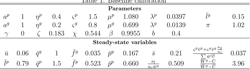
Table 1: Baseline calibration
Parameters
ap 1 ηp 0.4 ςp 1.5 µp 1.080 λp 0.0397 ¯lg 0.15
ag 1 ηg 0.2 ςg 0.8 µg 0.699 λg 0.0139 π 1.02
γ 0 ζ 0.183 χ 0.544 β 0.9955 b 0.4
Steady-state variables
¯
u 0.06 q¯g 1 f¯g 0.035 p¯g 0.167 s¯ 0.21 ς
pv¯p+ςgv¯g ug uc
P
¯
wi¯li 0.037
¯
lp 0.79 q¯p 1.5 f¯p 0.523 p¯p 0.660 νl
ucw¯g 0.509
¯
Wg−U¯ ¯
Wp−U¯ 3.96
set public sector matching elasticity with respect to unemployment, ηg at 0.15 and ηp at
0.4, slightly higher than the estimated value but in line with estimates from the literature
(Petrongolo and Pissarides (2001)). Elasticity with respect to vacancies of 0.85 in the public
sector is less extreme than in Quadrini and Trigari (2007). They use the minimum of
vacancies and unemployment as a matching function, which implies a matching elasticity of
1.
A recent paper by Davis, Faberman, and Haltiwanger (2013) provides some insights into
the duration of vacancies by sector. They use JOLTS data to study the behaviour of vacancies
and hiring. After adjusting the data, they estimate that government vacancy remains open
for 30 days while a private sector vacancy remains unfilled for only 20 days. I calibrate the
matching efficiency µi to reproduce these numbers (¯qp = 1 and ¯qg = 1.5).
Although I could not find data on public sector recruitment costs in the United States, the United Kingdom has a unique source. Every year, the Chartered Institute of Personal
Development performs a recruitment practice survey covering approximately 800
organi-zations from the following sectors: manufacturing and production, private sector services,
public sector services and voluntary, community and not-for-profit sector (CIPD (2009)).
The costs of recruiting a worker, which encompass advertising and agency costs, are
approx-imately £4000 for the median firm, corresponding to approximately 8 weeks of the median
income in the United Kingdom. On an average, these costs are 40 percent lower in the public
sector. I consider that these values indicate that cost per hire is lower in the public sector. I
consider the cost of posting a vacancy ςi to be 1.5 in the private sector and 0.8 in the public
sector. Given that a vacancy’s duration is longer in the public sector, these values imply
that the public sector’s average cost of recruiting expressed in the same units is 20 percent
lower than in the private sector. Under this calibration, recruitment costs total 3.7 percent
of total labour costs, close to the value found in Russo, Hassink, and Gorter (2005). These
numbers also imply that public vacancies are only 10 percent of private sector vacancies,
The empirical evidence relative to the substitution elasticity between private and govern-ment consumption is not conclusive. Evans and Karras (1998) find that private consumption
is complementary to military expenditure and a substitute for non-military expenditure.
Fiorito and Kollintzas (2004) disaggregate expenditure into ‘public goods’ (defence, public
order and justice) and ‘merit goods’ (health, education and other services). They find that
‘public goods’ are substitutes and ‘merit goods’ are complements to private consumption. In
the baseline case, I consider an elasticity of substitution of 1 (γ = 0.0), but also discuss the
cases where goods are substitutes (γ = 0.5) and complements (γ =−0.5). The parameterζ,
which reflects the preference for government services, is chosen such that the optimal level
of public sector employment is 0.15.
For the model to satisfy the Hosios condition in the private sector, the worker’s share in
the Nash bargaining is set at 0.4. The value of leisure in the utility function is calibrated
such that the steady-state unemployment rate is 0.06, implying an outside option equivalent
to 50 percent of the average wage. Technology in both sectors is normalised to 1 and the
discount factor is set at 0.9955, which implies an annual interest rate of 5 percent. Table 1
summarises the baseline calibration and the implied steady-state values for the key variables.
4
Optimal public sector wage in steady state
As already shown, the optimal wage ratio primarily depends on the difference between friction
parameters in the public and private sectors and only equals one if the sectors are symmetric.
Under the baseline calibration, the optimal public sector wage is 2.5 percent lower than in
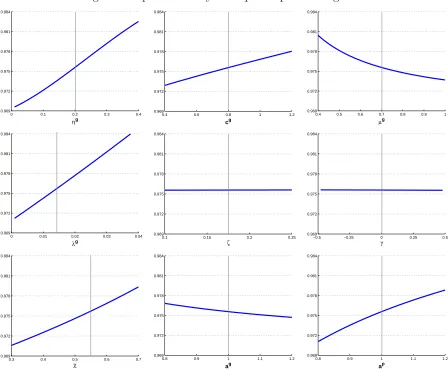
the private sector. Figure 3 shows how this optimal wage varies with the public sector’s
parameters.6
When the cost of posting vacancies is lower or when matching depends more on vacancies
(lower ηg), it is more efficient for the matching to be driven by vacancies rather than by
the unemployed. In order to induce fewer unemployed to search in the public sector, the
government should pay less to its workers. When the separation rate decreases or matching
becomes more efficient, more unemployed turn to the public sector at a time when it would
be optimal to have less. As the private incentive is not efficient, the government should
offer lower wages to correct this. Quantitatively, the difference between matching elasticities
6The companion appendix shows how the optimal share of unemployed searching in the two sectors,
Figure 3: Optimal steady-state public-private wage ratio
0 0.1 0.2 0.3 0.4 0.969 0.972 0.975 0.978 0.981 0.984 ηg
0.4 0.6 0.8 1 1.2 0.969 0.972 0.975 0.978 0.981 0.984 cg
0.4 0.5 0.6 0.7 0.8 0.9 1 0.969 0.972 0.975 0.978 0.981 0.984 µg
0 0.01 0.02 0.03 0.04 0.969 0.972 0.975 0.978 0.981 0.984 λg
0.1 0.15 0.2 0.25 0.969 0.972 0.975 0.978 0.981 0.984
ζ −0.5 −0.25 0 0.25 0.5
0.969 0.972 0.975 0.978 0.981 0.984 γ
0.3 0.4 0.5 0.6 0.7 0.969 0.972 0.975 0.978 0.981 0.984 χ
0.8 0.9 1 1.1 1.2 0.969 0.972 0.975 0.978 0.981 0.984 ag
0.8 0.9 1 1.1 1.2 0.969 0.972 0.975 0.978 0.981 0.984 ap
explains one third of the optimal public sector wage gap, while differences in separation rates
and vacancy-posting costs account for one sixth each.
The optimal wage ratio positively depends on the disutility of working (χ) and negatively
on the productivity of the public sector, but it does not depend on the coefficients of the
utility function, namely γ and ζ. Higher χ raises the value of employment in the private
sector relative to that in the public sector because people are more likely to have another
spell of unemployment if they are employed in the private sector. As this induces more
unemployed to search in the private sector, the government needs to offer higher wages to offset this preference.
In the numerical simulations, the cost of posting vacancies is not proportional to
produc-tivity. In such a scenario, lower productivity in the public sector indicates that the relative
cost of posting vacancies is higher because the marginal utility of public sector goods
public sector goods, it prefers new matches be driven by the unemployment side to save vacancy posting costs, a decision which requires higher public sector wages.
The parameters of the utility function mainly affect the optimal amount of public sector
goods produced, but numerically the parameters do not change the optimal wage ratio.
This result occurs because the optimal tightness in the two sectors stays the same, and the
different values of working in each sector as well as the value of being unemployed all remain
unchanged. As in the frictionless world, preferences determine the relative employment level
but not the wage ratio.
To investigate the consequences of paying more to public sector employees, I compare the unemployment rate when the public sector wage is optimal (a gap of 2.5 percent) with
the baseline case (a premium of 2 percent). The unemployment rate, which was calibrated
to 6 percent in the baseline steady state, falls to 5 percent when the government sets the
optimal wage. This happens because many unemployed that were queuing for public sector
jobs now find it more attractive to search in the private sector (¯s changes from 21 to 3
percent), boosting job creation. Interestingly, private sector wages do not go up in line
with public sector wages. On one hand, the public sector wages increase an unemployed’s
outside options if they search in the public sector, exerting an upward pressure on the wage
bargaining. On the other hand, such public sector wage increases also entail a negative wealth effect in the real business cycle sense. By increasing unemployment and crowding out
private employment permanently, they reduce the total amount of private goods produced in
the economy, raising their marginal utility. Higher marginal utility of consumption reduces
the value of being unemployed and makes people willing to work at lower wages. The second
effect seems to dominate. Welfare costs in the baseline scenario are equivalent to a permanent
private consumption reduction of 0.6 percent. All in all, public sector wages are an important
determinant of equilibrium unemployment.7
5
Public sector policies and the business cycle
Now I examine the effects of a 1 percent negative private technology shock on the
econ-omy under alternative government policies. I consider an AR(1) shock with autoregressive
coefficient ρ= 0.9.
ln(apt) = (1−ρ) ln(¯ap) +ρln(apt−1) +at.
Figure 4 shows the impulse responses, starting from the efficient steady state, when the government follows the optimal rule. I contrast the optimal policy with the following simple
rules for vacancies and wages:
log(vgt) = log(¯vg) +ψv[log(vpt)−log(¯vp)], (25)
log(wtg+1) = log( ¯wg) +ψw[log(wtp)−log( ¯wp)]. (26)
Existing evidence by Lane (2003) and Lamo, P´erez, and Schuknecht (2008) suggest that
public sector wages are less procyclical than private sector wages, particularly in the United
States.8 For simplicity, I consider two cases where public sector wages are acyclical (ψw = 0).
In the first case, public sector vacancies proportionally decline to increases in private sector
vacancies (ψv =−1). In the second, they are acyclical (ψv = 0).
After the negative productivity shock, private sector firms post fewer vacancies, resulting
in reduced probability of finding a job in this sector; therefore, the unemployed increasingly
search for public sector jobs. The unemployment rate increases at most by 0.06 percentage
points. As pointed out by Shimer (2005), under a standard calibration, search and matching
models cannot generate sufficient fluctuations in unemployment in response to technology
shocks.
Optimal government policy will have procyclical wages and counter-cyclical vacancies.
The sector reallocation argument advocates hiring more people in recessions. If the private sector has lower productivity, the economy will be better served by the public sector
ab-sorbing part of the unused labour force. This result is fragile in two dimensions. First, it
depends on preferences. Figure 5 shows the optimal business cycle policy for three cases: if
the goods are substitutes (γ = 0.5), complements (γ =−0.5) and the baseline case with an
elasticity of substitution of 1 (γ = 0.0). The result is overturned if the goods are strong
com-plements. In this case, during a recession, as the marginal utility of the government services
falls with consumption of private goods, the government should also reduce the number of
people it employs. The result of counter-cyclical vacancies also breaks down following an
economy-wide technological shock or discount factor shocks. As they affect both sectors
symmetrically, the argument for sector reallocation no longer holds.9
On the other hand, public sector wages should follow declines in private sector wages. In
recessions, if the government keeps its wages constant, it becomes more attractive relative
8Additionally, a study by Devereux and Hart (2006) using micro data for the United Kingdom finds that
for job movers in the private sector, the wages are procyclical but for the public sector they are acyclical.
Figure 4: Response to a private sector technology shock under different policies
0 10 20 30 40 50 60 −0.02 −0.01 0 0.01 0.02 0.03 0.04 0.05 0.06 0.07 Unemployment Rate Months %
0 10 20 30 40 50 60 −0.45 −0.4 −0.35 −0.3 −0.25 −0.2 −0.15 −0.1 −0.05 0 Private Employment Months %
0 10 20 30 40 50 60 0 0.5 1 1.5 2 2.5 Public Employment Months %
0 10 20 30 40 50 60 −0.2 0 0.2 0.4 0.6 0.8 1 1.2 1.4 1.6 1.8
Share of unemployed searching for lg
Months
%
0 10 20 30 40 50 60 −1.4 −1.2 −1 −0.8 −0.6 −0.4 −0.2 0
Private sector wage
Months
%
0 10 20 30 40 50 60 −1.4 −1.2 −1 −0.8 −0.6 −0.4 −0.2 0
Public sector wage
Months
%
0 10 20 30 40 50 60 −3 −2.5 −2 −1.5 −1 −0.5 0
Vacancies − private sector
Months
%
0 10 20 30 40 50 60 −0.5 0 0.5 1 1.5 2 2.5 3
Vacancies − public sector
Months
%
0 10 20 30 40 50 60 −1 −0.5 0 0.5 1 1.5 2 2.5 Government spending Months %
Note: Solid line (optimal policy); dash line (counter-cyclical vacancies and acyclical wages) and dotted line (acyclical vacancies and wages). The response of the variables is shown in percentage of their steady-state value, except for unemployment rate and the share of unemployed searching for public sector jobs, which is expressed in percentage point difference from the steady state.
to the private sector, thus increasing the share of unemployed searching for public sector
jobs. This in turn reduces the probability that a vacancy in the private sector will be filled,
which further dampens job creation and amplifies the business cycle. We can see that under
the two exogenous rules, unemployment shows a much stronger response. The share of
unemployed searching of public sector jobs increases by 1.6 percentage points, much higher
than under the optimal policy (0.02 percentage points). This result is remarkably robust to
alternative preference specifications or business cycle driving forces. This robustness reflects
Figure 5: Optimal business cycle policy under different elasticities
0 10 20 30 40 50 60 −0.005 0 0.005 0.01 0.015 0.02 0.025 0.03 0.035 Unemployment Rate Months %
0 10 20 30 40 50 60 −0.16 −0.14 −0.12 −0.1 −0.08 −0.06 −0.04 −0.02 0 0.02 Private Employment Months %
0 10 20 30 40 50 60 −0.2 −0.1 0 0.1 0.2 0.3 0.4 0.5 0.6 0.7 Public Employment Months %
0 10 20 30 40 50 60 −0.4 −0.2 0 0.2 0.4 0.6 0.8 1
Share of unemployed searching for lg
Months
%
0 10 20 30 40 50 60 −1.4 −1.2 −1 −0.8 −0.6 −0.4 −0.2 0
Private sector wage
Months
%
0 10 20 30 40 50 60 −1.4 −1.2 −1 −0.8 −0.6 −0.4 −0.2 0
Public sector wage
Months
%
0 10 20 30 40 50 60 −2 −1.8 −1.6 −1.4 −1.2 −1 −0.8 −0.6 −0.4 −0.2 0
Vacancies − private sector
Months
%
0 10 20 30 40 50 60 −10 −5 0 5 10 15 20 25
Vacancies − public sector
Months
%
0 10 20 30 40 50 60 −1.4 −1.2 −1 −0.8 −0.6 −0.4 −0.2 0 Government spending Months %
Note: Solid line (γ= 0.0); dash line (substitutes, γ= 0.5) and dotted line (complements, γ=−0.5). The response of the variables is expressed in percentage of their steady-state value, except for unemployment rate and the share of unemployed searching for public sector jobs, which is shown in percentage point difference from the steady state.
comovement.10
Table 2 compares the standard deviation of key variables in the alternative policies, as
well as when no public sector exists (ζ = 0). If government follows the optimal policy, the
presence of public sector employment stabilises unemployment. However, if public sector
wages are acyclical, unemployment volatility increases twofold.
In their paper, Quadrini and Trigari (2007) have two conclusions contrary to mine. First, they argue that the presence of the public sector increases unemployment volatility. I show
10Optimal wage policy would be reinforced with endogenous job destruction. In recessions, the
Table 2: Business cycle properties under different policies
Policy Standard deviations Correl Welfare
lpt lgt ut wpt (l g
t, ut) cost
Optimal steady-state wage
No government 0.0008 − 0.0007 0.021 − 0.022%
Optimal policy 0.0008 0.0004 0.0006 0.021 0.994 0.018%
Rule (ψw = 0, ψv =−1) 0.0282 0.1558 0.0016 0.0206 −0.506 0.296%
Rule (ψw = 0, ψv = 0) 0.0247 0.1350 0.0015 0.0206 −0.368 0.240%
Optimal steady-state wage Substitutes (γ = 0.5)
Optimal policy 0.0035 0.0157 0.0005 0.021 0.919 0.0186%
Rule (ψw = 0, ψv =−1) 0.0274 0.1482 0.0015 0.0207 −0.252 0.184%
Rule (ψw = 0, ψv = 0) 0.0233 0.1249 0.0014 0.0208 −0.084 0.150%
Complements (γ =−0.5)
Optimal policy 0.0002 0.0047 0.0007 0.021 −0.985 0.0231%
Rule (ψw = 0, ψv =−1) 0.0292 0.1645 0.0019 0.0205 −0.695 0.553%
Rule (ψw = 0, ψv = 0) 0.0263 0.1473 0.0017 0.0205 −0.612 0.463%
Baseline steady-state wage
Rule (ψw = 1, ψv =−1) 0.0015 0.0051 0.0007 0.021 0.498 −
Rule (ψw = 0, ψv =−1) 0.0060 0.0218 0.0022 0.021 0.473 −
Rule (ψw = 0, ψv = 0) 0.0047 0.0147 0.0022 0.021 0.480 −
that this result is not general and that the presence of public sector employment affects
unemployment volatility in a manner crucially dependant on the government’s business cycle policy. Second, they argue that procyclical public sector employment is the best policy to
stabilize total employment, but this is not the optimal policy. In their model, the government
does not choose wages optimally, in either the steady state or along the business cycle.
Procyclical employment can be optimal if public sector wages are not. But if they are,
public sector vacancies and employment should be counter-cyclical.
The last column presents the welfare cost of business cycles in the different scenarios.11
When the public sector is absent, fluctuations have a very small welfare cost –
approxi-mately 0.028 percent of steady-state consumption. This is a well known result. When the
government is present and behaves optimally, the fluctuations have lower welfare costs, but under the two rules, the cost can be up to four times higher. Welfare costs are higher when
the goods are complements, as a negative technology shock has further negative effects on
the marginal utility of the public good. Optimal business cycle policy requires the policy
to remain optimal in the steady state. Outside the efficient steady state, characterizing the
optimal business cycle policy is difficult, but we can analyse the volatility of key variables
depending on business cycle policy. The last panel of Table 2 shows the case for the base-line steady state. In the two scenarios with acyclical public sector wages, unemployment
volatility is three times higher than when the public sector wages respond one-to-one to the
private sector.
In a final robustness exercise, I investigate if these conclusions change in the presence of
rigid private sector wages. I considered two alternative methods of modelling: one following
Hall (2005) and the second following Blanchard and Gal´ı (2010). In both cases, rigidities are
introduced by assuming an ad-hoc expression for wages. Full details and results are shown
in the companion appendix. Compared to the flexible wage benchmark, unemployment rate
volatility increases three times in the case of Hall (2005) specification and 15 times in the case of Blanchard and Gal´ı (2010). In both cases, we observe reduced unemployment volatility
when government follows a procyclical wage policy, but by less than the benchmark case.
The standard deviation of unemployment rate decreases by only 10 percent. Rigid wages
reduce the cost of not following a procyclical public wage policy. Although wage rigidity has
been proposed in the literature as one solution to the Shimer Puzzle, its relevance is still
under discussion. For the main mechanism of the model, only the wages of new-hires are
relevant in the decisions. As been argued by Pissarides (2009), microeconometric evidence
suggests that wages in new matches are more procyclical and volatile than average wages.
6
Directed versus random search
6.1
Evidence for Directed search
The theoretical model presented in this paper has two important policy prescriptions. First,
government wages in the steady state should not be too high relative to the private
sec-tor. Otherwise they generate higher equilibrium unemployment. Second, government wages
should track private sector wages over the business cycle or unemployment volatility will be
higher due to fluctuations in the share of unemployed searching for public sector jobs. An
important part of the mechanism depends on the assumption of directed search.
According to micro evidence, this assumption is very realistic. As mentioned previously,
public sector wage premium substantially varies within groups. As reported in Gregory and
Borland (1999), the premium is much higher for females, veterans and minorities, and is
higher for federal government employees compared to state or local government employees.
Differences also exist across education levels. Katz and Krueger (1991) find that in the
while individuals with less education tend to receive a higher premium. If people can direct their search, these differences should have repercussions.
Gregory and Borland (1999) report a number of studies that found the existence of queues
for federal public jobs. For example, Venti (1985) finds that for each federal government job
opening, 2.8 men and 6.1 times as many women want the job. Katz and Krueger (1991)
find that blue collar workers are willing to queue to obtain public sector jobs, whereas the public sector has difficulty in recruiting and retaining highly skilled workers. Postel-Vinay
and Turon (2007) also finds evidence in the United Kingdom of low-employability individuals
queuing for public sector jobs, as they stand to gain larger potential premia from working
there.
Most studies that estimate the public sector wage premium use switching regression
models, which posit that the unemployed can self-select to work in the sectors offering more
advantages. Blank (1985) finds that, among other factors, sectoral choice is influenced by
wage comparison. Heitmueller (2006) manages to quantify this effect and finds that an
in-crease of 1 percent in the public sector’s expected wage inin-creases the probability employment
in that sector by 1.3 percent for men and 2.9 percent for women.
The micro evidence supports the directed search assumption in the steady state. However,
over the business cycle, as the public sector premium is different for subgroups based on
characteristics that do not change over the cycle, small changes in private sector wages might
not be sufficient to change aggregate search patterns. Note that the successful functioning
of this mechanism does not require every unemployed to swing between sectors, as long as a
small number at the margin are so able. Anecdotal evidence presented in the introduction
already suggests that the same mechanism is also relevant over the business cycle.
6.2
The case with random search
Although directed search is an important part of the mechanism, the main results are also
robust if we consider search as being random. Consider the following specification in which
the unemployed do not have a choice where to search:
mpt +mgt =µ(ut)η(vpt +v g t)
1−η, (27)
vtg vtp =
mgt
mpt. (28)
There is one matching function that has unemployment and the total number of vacancies
function, only public sector vacancies. However, public sector wages still affect the value of unemployment and, hence, the outside option of the worker when bargaining.
Ut =
νu(ut)
uc(ct, gt)
+Etβt,t+1[ftpW p t+1+f
g tW
g
t+1+ (1−f
g t −f
p
t)Ut+1]. (29)
In this setting, optimality only requires optimal vacancies in both sectors. The government
can set the optimal level of government vacancies directly, incorporating the resulting
exter-nality. As there is one less variable for efficiency, the government can now use public sector
wages as an instrument to achieve the optimal level of private vacancies. This means that,
for any bargaining power of the worker (even if the Hosios condition is not satisfied), only
one public sector wage will achieve the optimal level of private sector vacancies. As with
directed search, higher public sector wages imply both higher wages and lower vacancies in the private sector, and hence higher unemployment. This is also true over the business
cycle. Unemployment volatility is higher if public wages are kept constant. In essence,
di-rected search amplifies the costs of not following the optimal policy through the endogenous
decision of where to search.12
7
Conclusion
This paper examines the links between public and the private sectors through the labour
market. The main normative conclusion is that government wage policy plays a key role in
attaining efficient allocation of jobs across sectors. In the steady state, the optimal public
sector wage premium should reflect differences in labour market friction parameters.
Al-though other reasons exist for governments to set wages, namely to induce effort or avoid corruption, they should weigh the cost of such an action in terms of labour market
ineffi-ciency, as higher wages relative to the private sector induce queues and higher equilibrium
unemployment.
Over the business cycle, public sector wages should follow those in the private sector.
Otherwise, in recessions, too many people queue for public sector jobs whilst in expansions,
few people apply for them. Although I have abstracted from financing issues, a procyclical
public sector wage has the advantage of requiring a lower tax burden in recessions.
How-ever, it also has drawbacks. First, lowering public sector wages in recessions might prove
politically difficult to implement. Yet, to achieve efficiency in the labour market, the only
relevant wages are those of new hires, which are potentially easier to reduce in recessions.
12In the companion appendix, I present details of the model with random search, the social planner
Second, it does not seem plausible that government can vary wage from quarter to quarter. However, indexing annual wage increases to the evolution of their private sector counterparts
is possible. Finally, I have ignored the insurance role of the government. If agents are risk
averse, they would prefer to have a constant income profile throughout the business cycle,
which is an argument for acyclical wages. While this line of reasoning is valid, one has to
realise that the intertemporal insurance is achieved at the cost of greater fluctuations in
unemployment.
The results on optimal policy are relevant in two ways. First, studies of optimality in
fiscal policy have primarily focused on the taxation side because on the spending side, it is
harder to dissociate optimal policy from preferences. In the model, government policy on vacancies and employment faces the same problem, which is why I give it little relevance. On
the other hand, the results of government wages essentially depend on the labour market,
which allow us to develop a more robust theory of optimal spending, at least for one of its
components.
The result is considered relevant because despite being simple and intuitive, optimal
busi-ness cycle policy does not seem to be acknowledged by policy makers who view government
wages as a stabilization tool. In a recent occasional paper from the European Central Bank
(Holm-Hadulla, Kamath, Lamo, P´erez, and Schuknecht (2010)), the authors argue that the
government should avoid mild wage procyclicality, as increasing wages in expansions might
boost aggregate demand and amplify the business cycle. As we have seen, this policy could
heavily distort the labour market. To stabilise demand, the government can use either
em-ployment, purchases of intermediate goods, investment or transfers, but leave the wage to
promote efficiency in the labour market.
References
Albrecht, J., L. Navarro, and S. Vroman (2013): “Public Sector Employment in an
Equilibrium Search and Matching Model,” Discussion paper.
Ardagna, S. (2007): “Fiscal policy in unionized labor markets,” Journal of Economic
Dynamics and Control, 31(5), 1498–1534.
Barro, R. J. (1990): “Government Spending in a Simple Model of Endogenous Growth,”
Baxter, M., and R. G. King (1993): “Fiscal Policy in General Equilibrium,” American
Economic Review, 83(3), 315–34.
Blanchard, O., and J. Gal´ı (2010): “Labor Markets and Monetary Policy: A New
Keynesian Model with Unemployment,” American Economic Journal: Macroeconomics,
2(2), 1–30.
Blank, R. M. (1985): “An analysis of workers’ choice between employment in the public
and private sectors,”Industrial and Labor Relations Review, 38(2), 211–224.
Bradley, J., F. Postel-Vinay, and H. Turon (2013): “Public sector wage policy and
labour market equilibrium: a structural model,” Discussion paper.
Burdett, K. (2012): “Towards a theory of the labor market with a public sector,”Labour
economics, 19(1), 68–75.
Burdett, K., and D. T. Mortensen (1998): “Wage Differentials, Employer Size, and
Unemployment,”International Economic Review, 39(2), 257–73.
CIPD (2009): “Recruitment, retention and turnover survey report,” Available at
http://www.cipd.co.uk/subjects/recruitmen/general/.
Davis, S. J., R. J. Faberman, and J. C. Haltiwanger (2013): “The
Establishment-Level Behavior of Vacancies and Hiring,” The Quarterly Journal of Economics, 128(2),
581–622.
Devereux, P. J., and R. A. Hart (2006): “Real wage cyclicality of job stayers,
within-company job movers, and between-within-company job movers,” Industrial and Labor Relations
Review, 60(1), 105–119.
Evans, P., and G. Karras (1998): “Liquidity Constraints and the Substitutability
be-tween Private and Government Consumption: The Role of Military and Non-military
Spending,” Economic Inquiry, 36(2), 203–14.
Finn, M. G.(1998): “Cyclical Effects of Government’s Employment and Goods Purchases,”
International Economic Review, 39(3), 635–57.
Fiorito, R., and T. Kollintzas (2004): “Public goods, merit goods, and the relation
between private and government consumption,”European Economic Review, 48(6), 1367–
Gal´ı, J., J. D. L´opez-Salido, and J. Vall´es (2007): “Understanding the Effects of
Government Spending on Consumption,”Journal of the European Economic Association,
5(1), 227–270.
Gregory, R. G., and J. Borland (1999): “Recent developments in public sector labor
markets,” in Handbook of Labor Economics, ed. by O. Ashenfelter, and D. Card, vol. 3,
chap. 53, pp. 3573–3630. Elsevier.
Hall, R. E.(2005): “Employment Fluctuations with Equilibrium Wage Stickiness,”
Amer-ican Economic Review, 95(1), 50–65.
Heitmueller, A. (2006): “Public-private sector pay differentials in a devolved Scotland,”
Journal of Applied Economics, IX, 295–323.
Holm-Hadulla, F., K. Kamath, A. Lamo, J. J. P´erez,and L. Schuknecht(2010):
“Public wages in the euro area - towards securing stability and competitiveness,”
Occa-sional Paper Series 112, European Central Bank.
Holmlund, B., and J. Linden (1993): “Job matching, temporary public employment,
and equilibrium unemployment,”Journal of Public Economics, 51(3), 329–343.
H¨orner, J., L. R. Ngai, and C. Olivetti (2007): “Public Enterprises And Labor
Market Performance,” International Economic Review, 48(2), 363–384.
Katz, L. F., and A. B. Krueger (1991): “Changes in the Structure of Wages in the
Public and Private Sectors,” NBER Working Papers 3667.
Lamo, A., J. J. P´erez, and L. Schuknecht(2008): “Public and private sector wages
-co-movement and causality,” Working Paper Series 963, European Central Bank.
Lane, P. R. (2003): “The cyclical behaviour of fiscal policy: evidence from the OECD,”
Journal of Public Economics, 87(12), 2661–2675.
Linnemann, L., and A. Schabert (2003): “Fiscal Policy in the New Neoclassical
Syn-thesis,”Journal of Money, Credit and Banking, 35(6), 911–29.
Merz, M. (1995): “Search in the labor market and the real business cycle,” Journal of
Monetary Economics, 36(2), 269–300.
Pappa, E. (2009): “The Effects Of Fiscal Shocks On Employment And The Real Wage,”
Petrongolo, B., and C. A. Pissarides (2001): “Looking into the Black Box: A Survey
of the Matching Function,” Journal of Economic Literature, 39(2), 390–431.
Pissarides, C. A. (2000): Equilibrium unemployment. MIT press, 2nd edn.
Pissarides, C. A. (2009): “The Unemployment Volatility Puzzle: Is Wage Stickiness the
Answer?,”Econometrica, 77(5), 1339–1369.
Postel-Vinay, F., and H. Turon (2007): “The Public Pay Gap in Britain: Small
Dif-ferences That (Don’t?) Matter,”Economic Journal, 117(523), 1460–1503.
Quadrini, V., and A. Trigari (2007): “Public Employment and the Business Cycle,”
Scandinavian Journal of Economics, 109(4), 723–742.
Russo, G., W. Hassink,andC. Gorter(2005): “Filling vacancies: an empirical analysis
of the cost and benefit of search in the labour market,”Applied Economics, 37(14), 1597–
1606.
Shimer, R.(2005): “The Cyclical Behavior of Equilibrium Unemployment and Vacancies,”
American Economic Review, 95(1), 25–49.
COMPANION APPENDIX
FOR ONLINE PUBLICATION
Optimal public sector wages
Pedro Gomes
I - Data
• Table A1: Public sector and the labour market in OECD countries
• Table A2: Data on cost of recruiting - CIPD
• Figure A1: Growth rate of Google keyword searches in the United Kingdom
II - Steady-state optimal wages, search and unemployment
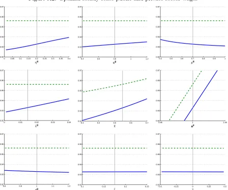
• Figure A2: Optimal steady-state public and private sector wages
• Figure A3: Optimal steady-state public and private sector tightness
• Figure A4: Optimal steady-state share of unemployed searching in public sector
• Figure A5: Optimal steady-state level of public sector employment
• Figure A6: Optimal steady-state unemployment rate
• Figure A7: Cost of higher public sector wages
III - Optimal policy under alternatives sources of fluctuations
• Figure A8: Optimal business cycle policy under an economy wide technology shock
• Figure A9: Optimal business cycle policy under a discount factor shock
IV - Wage rigidity
• Two specifications
• Table A3: Business cycle properties with wage rigidity
V - Derivations
• Social planner’s problem
• Proof of proposition 1
• Welfare costs of high public sector wages
• Welfare costs of business cycles
VI - Model with random search
• Setting
• Social planner’s problem
• Figure A10: Optimal public-private wage ratio with random search