BIROn - Birkbeck Institutional Research Online
Hu, W. and Gao, J. and Xing, J. and Zhang, C. and Maybank, Stephen (2017)
Semi-supervised tensor-based graph embedding learning and its application
to visual discriminant tracking. IEEE Transactions on Pattern Analysis and
Machine Intelligence 39 (1), pp. 172-188. ISSN 0162-8828.
Downloaded from:
Usage Guidelines:
Please refer to usage guidelines at or alternatively
Semi-Supervised Tensor-Based Graph Embedding Learning
and Its Application to Visual Discriminant Tracking
Weiming Hu, Jin Gao, Junliang Xing, and Chao Zhang
(CAS Center for Excellence in Brain Science and Intelligence Technology, National Laboratory of Pattern Recognition, Institute of Automation, Chinese Academy of Sciences, Beijing 100190)
{wmhu, jin.gao, jlxing}@nlpr.ia.ac.cn; [email protected] Stephen Maybank
(Department of Computer Science and Information Systems, Birkbeck College, Malet Street, London WC1E 7HX) [email protected]
Abstract: An appearance model adaptable to changes in object appearance is critical in visual object tracking. In this paper, we treat an image patch as a 2-order tensor which preserves the original image structure. We design two graphs for characterizing the intrinsic local geometrical structure of the tensor samples of the object and the background. Graph embedding is used to reduce the dimensions of the tensors while preserving the structure of the graphs. Then, a discriminant embedding space is constructed. We prove two propositions for finding the transformation matrices which are used to map the original tensor samples to the tensor-based graph embedding space. In order to encode more discriminant information in the embedding space, we propose a transfer-learning- based semi-supervised strategy to iteratively adjust the embedding space into which discriminative information obtained from earlier times is transferred. We apply the proposed semi-supervised tensor-based graph embedding learning algorithm to visual tracking. The new tracking algorithm captures an object’s appearance characteristics during tracking and uses a particle filter to estimate the optimal object state. Experimental results on the CVPR 2013 benchmark dataset demonstrate the effectiveness of the proposed tracking algorithm.
Index terms: Discriminant tracking, Tensor samples, Semi-supervised learning, Graph embedding space
1. Introduction
models can be categorized into generative models and discriminative models [45]. A generative model describes the distribution of the image patches of an object in previous frames. Tracking is reduced to a search for an optimal state that yields an object appearance most similar to the model. A discriminative model describes not only the image patches of the object but also some background image patches. The tracking is based on a binary classifier to distinguish the object from the background. Usually, the image patches corresponding to the tracking results are used as the labeled positive samples, and the image regions selected from the background are used as the labeled negative samples [6, 10]. Then, a classifier is trained in a supervised way using these labeled positive and negative samples. A number of new samples can be selected in each new frame, and these unlabeled samples are used in a semi-supervised way [6, 10] to improve the classifier.
In this paper, we propose a new discriminative tracking algorithm in which each image patch is represented by a 2-order tensor. The relations among object image patches and background image patches in the previous frames are represented by graphs. The 2-order tensor-based graph embedding is used to learn the discriminative subspace (the discriminative embedding space) for distinguishing the object image patches from the background image patches. A number of unlabeled image patches collected from the current frame are used to refine the discriminative embedding space.
1.1. Related work
In order to give the context of our work, we briefly review image-as-vector representation, image-as-feature representation, and image-as-matrix representation for image patches, together with semi-supervised strategies for discriminant tracking.
1) Image-as-vector representation: Many tracking algorithms [21, 35] adopt a holistic image-as-vector representation in which image patches are flattened to vectors. These algorithms include 1 minimization- based tracking algorithms [3, 17, 18, 33, 34], which exploit the sparse representation of image patches on the object. Kwon and Li [8, 9] constructed multiple basic appearance models using sparse principal component analysis (PCA) of a set of feature templates, such as global image-as-vector descriptors of hue, saturation, intensity, and edge information. These image-as-vector representation methods ignore the fact that an image is intrinsically a matrix or a 2-order tensor, and thus mask the underlying 2D structure of an image. This may lead to the loss of the discriminant information required for tracking.
2) Image-as-feature representation: There are algorithms that directly extract features from image patches and use the features to carry out tracking. For instance, Grabner et al. [5, 6] used Haar-like features, histograms of oriented gradients, and local binary patterns to obtain weak hypotheses for boosting-based tracking. In [2, 10] only Haar-like features were used, but great improvements were achieved by novel appearance models. Li et al.
histogram features. Although image-as-feature representations, such as Haar-like featured-based ones, are appropriate for specifically designed discriminant learning methods, such as boosting, a lot of useful information is omitted from the features.
3) Image-as-matrix presentation: image-as-matrix representation, such as tensor representation, retains much more useful information because the original image structure is preserved. It usually models the relations between pixel rows and the relations between pixel columns while the image-as-vector representation usually only models the relations between pixels. Tensor-based subspace learning [7, 27, 29] has been applied to visual tracking [11, 13, 24, 25, 26]. Some tensor-based tracking algorithms [13, 24, 25] conducted PCA on the mode-k
unfolding matrix. There are algorithms [11, 26] in which eigenvalue decomposition on the covariance [19] in the mode-k unfolding matrix was applied to carry out tracking tasks. Although these tensor-based tracking methods take into account the correlations between different dimensions of the object appearance which changes over time, they currently have the following limitations:
The dimension reduction-based subspace learning methods used in [13, 24, 25] have the problem of subspace learning degradations [27] which may lead to loss of tracking. Although Yan et al. [27] proposed to rearrange pixels in the tensor to deal with subspace learning degradation, the time consuming pixel rearrangement is unsuitable for tracking applications.
The current tensor-based tracking algorithms cannot fully detect the intrinsic local geometrical and discriminative structure of the collected image patches in tensor form.
The current tensor-based tracking algorithms ignore the influence of the background and consequently suffer from distractions caused by background regions with appearances similar to the object.
Two-dimensional linear discriminant analysis (2DLDA) [30] was proposed to detect the discriminative structure of 2-order tensor samples. However, the intrinsic local geometrical structure of the samples cannot be detected, because 2DLDA does not take into account the variations in the samples within the same class.
useful for improving the classifier, it is required to select useful unlabeled samples and assign correct class labels to them. Bennett et al. [4] and Rosenberg et al. [20] proposed the classification margin improvement techniques [4, 20] to select the unlabeled samples with the highest classification confidences. These unlabeled samples were assigned with the class labels that are predicted by the current classifier. These techniques may increase the classification margin, but they do not provide any novel information to adjust the discriminative subspace. The margin improvement techniques are inappropriate for visual tracking.
1.2. Our work
[image:5.595.91.502.418.518.2]Graph embedding for dimension reduction [22, 28] provides a new framework to handle the limitations in the image-as-matrix representations. In this paper, we propose a semi-supervised tensor-based graph embedding learning algorithm and apply it to visual discriminant tracking [38]. Fig. 1 shows the high level framework for our tracker. Our algorithm treats an image patch as a 2-order tensor. The labeled object and background tensor samples collected in previous frames and the unlabeled tensor samples collected in the current frame are used to train a tensor-based graph embedding space by our proposed semi-supervised graph embedding learning algorithm. This graph embedding algorithm is incorporated into the particle filtering-based tracking framework to track the object in the current frame. The tracking result in the current frame is used to update the set of the labeled samples.
Fig. 1. The high level framework for our tracker.
In our 2-order tensor-based graph embedding learning algorithm, an intrinsic graph is designed to represent correlations between the object tensor samples and correlations between the background tensor samples. A penalty graph is designed to keep apart the object tensor samples and the background tensor samples. The framework of graph embedding for dimension reduction is used to find the transformation matrices for mapping the original tensor samples to the tensor-based graph embedding space. Due to the degradations in the tensor embedding space learning [27], the embedding may not contain enough discriminative information for reliable tracking. We propose to encode more discriminant information by improving the tensor-based discriminative embedding space using the available unlabeled tensor samples in a semi-supervised way. In discriminant tracking, the existing single transformation matrix-based method [36] improves the discriminant space only by adding to the objective function a constraint term for handling the unlabeled samples. This method is difficult to use intuitively and directly in the 2-order tensor-based graph embedding learning for which two transformation
Labeled tensor samples
Unlabeled tensor samples
Semi-supervised tensor-based graph
embedding
Particle filtering tracking framework
The tracking result at the current frame Update the
matrices are required, because it is difficult to define an appropriate regularizer for handling the two associated transformation matrices. In this paper, we carry out a transfer-learning-based semi-supervised improvement in an iterative way. At each iteration, the unlabeled tensor samples which are most probably misclassified at the previous iteration are selected according to their similarities to the labeled samples which are collected at earlier tracking stages. The corrected class labels are assigned to the selected unlabeled samples and used to learn a new discriminative embedding space into which the information about the earlier changes in object appearance is transferred. The learned embedding spaces from different iterations are combined linearly to form a final adjusted embedding space.
The main contributions of our work are summarized as follows:
We develop a 2-order tensor-based graph embedding learning algorithm. The intrinsic local geometrical and discriminative structures of the tensor samples are effectively represented.
We propose a transfer-learning-based semi-supervised learning method to adjust the 2-order tensor graph embedding space. The semi-supervised technique selects the unlabeled tensor samples by comparing them with the samples with known classes collected at earlier times. Historical complementary information is transferred to adjust the discriminative embedding space.
We incorporate the proposed semi-supervised 2-order tensor-based graph embedding learning procedure into a Bayesian inference framework. Then, a new visual discriminative tracker is formed to effectively capture the appearance changes and reliably separate a moving object from the background. The remainder of the paper is organized as follows: Section 2 proposes our 2-order tensor-based graph embedding learning algorithm. Section 3 presents the transfer-learning-based semi-supervised improvement strategy. Section 4 describes our discriminant tracking algorithm. Section 5 demonstrates the experimental results. Section 6 summarizes the paper.
2. Tensor-Based Graph Embedding
In the following, we summarize the tensor operations, introduce the basic concept of tensor-based graph embedding, and propose our 2-order tensor-based graph embedding learning algorithm.
2.1. Tensor operations
A tensor [23] can be regarded as a multi-order “array” lying in multiplevector spaces. An n-order tensor is denoted as I1 I2 Ik In, where
k
I (k1, 2,..., )n is a positive integer. An element in the tensor is represented as ai1,...,ik,...,in, where 1 ik Ik. The inner product of two n-order tensors and is defined as:
1 2
1 2 1 2 1 2
, ,..., , ,..., 1 1 1
, ...
n
n n
n
I I I
i i i i i i
i i i
a b
. (1)F. The distance between and is .
Each order of a tensor is associated with a “mode”. Along a mode k, a tensor is unfolded into a matrix ( )
( )
k i ki
I I
k
A which consists of Ik-dimensional mode-k column vectors obtained by varying the k-th mode index ik and keeping the indices of the other modes fixed. The inverse of mode-k unfolding is mode-k folding, which restores the original tensor from A( )k . The mode-k product kM of a tensor and a matrix
M Jk Ik is a tensor I1 ...Ik1 Jk Ik1 ...In whose entries are:
1,..., 1, , 1,..., 1,..., 1, , 1,..., 1
, 1,...,
k
k k n k k n
I
i j i i i i i i i ji k
i
c a M j J
. (2)The tensor can also be obtained by matrix multiplication C( )k MA( )k and then mode-k folding of C( )k .
Given a tensor and three matrices Γ JnIn, Ψ KnJn, and Z JmIm (nm), the following tensor
mode-n product formulae hold ( nΓ)mZ( mZ)nΓ nΓmZ and ( nΓ)nΨ n(ΨΓ).
2.2. Tensor-based graph embedding
Let 1 2
1,2,..., { I I In}
i i N
be the set of N training samples in the n-order tensor form. An intrinsic graph and a penalty graph p
, both of which have the vertex set { i}i1,2,...,N, are constructed to model the local geometrical and discriminative structure of tensor samples. Let W and Wp
be the edge weight matrices of and p
, respectively. The entry Wij in W measures the similarity between vertices i and j, and the entry p
ij
W in Wp measures their difference. The intrinsic graph describes desired statistical or geometric properties of the samples. The penalty graph characterizes statistical or geometric properties to be suppressed. The graphs and p
are designed according to the application [40].
The task of the tensor-based graph embedding [28] is to find an optimal low dimensional tensor representation for each vertex in a graph such that the low dimensional tensor representations optimally characterize the similarities between the vertex pairs. The characteristics of the original intrinsic graph are preserved and at the same time the characteristics identified by the penalty graph are suppressed. Let
1,2,..., , {M kk} kk
k l I
k n l I be a set of n transformation matrices which map the samples { i}i1,2,...,N to N points
1 2 ... 1,2,..., { l l ln}
i i N
in a lower dimensional tensor subspace. Namely 1 2 1 2 ...
n
i i M M nM . Then, an optimal transformation which preserves the graph structure is obtained by solving the following optimization:
21 1 1 2 1 1 arg min subject to N N n k
i j ij
k
i j
N N
p
i j ij
where d is a constant.
2.3. Two order tensor-based graph embedding learning
In many applications, such as discriminant tracking, the samples can be expressed in the 2-order tensor form: 1 2
1,2,..., { I I }
i i N
, and the sample set consists of labeled training samples and unlabeled samples. The unlabeled samples are usually given pseudo labels which are predicted by a classifier. Let “ 1 ” indicate the labeled positive samples, and “ 1 ” indicate the labeled negative samples. Let “+2” indicate the pseudo positive samples, and “ 2 ” indicate the pseudo negative samples. Then, the class labels of the training samples are represented by { ,L ii 1, 2,..., }N (Li
2, 1, 1, 2 )
. Let nc be the number of the samples with class
2, 1, 1, 2
c . Then, 2
2
c nc N.The intrinsic graph in the graph embedding framework characterizes the intra-class compactness. The penalty graph characterizes the interclass separability. The distributions of samples, such as the background samples in tracking applications, are disordered, irregular, and multimodal. The global linking [36] between samples for defining the graph structure may not be effective for classes which are widely scattered. As a result, its ability to maximize the between-class scatters is limited. Local linking between samples for defining the graph structure is more appropriate to preserve the scattered sample distributions. In this paper, we design the two graphs, and p, to model the local geometrical and discriminative structure of the tensor samples.
2.3.1. Definition of graph structure
We define the affinity Aij between samples i and j using the local scaling method in [32]. Without loss of generality, we assume that the data points in
i Ni1 are ordered according to their labels { }Li(Li
2, 1, 1, 2
). When Li 0 and Lj0, Aij is defined as: 2exp i j ij i j A (4)
where i i i( )k , and ( )k
i is the k-th nearest neighbor of i in { } 2 1 1
N
j j nn . The affinities for a
positive or pseudo positive sample are defined for all the positive and pseudo positive samples. When Li 0 and Lj 0, Aij is defined as:
2
|| ||
exp , if ( ) or ( )
0, otherwise
i j
k k
ij i j
i N j j N i A
(5)
where N ik( ) is the index set of the k-nearest neighbors of i in
2 1 1 { }n n
j j , ( ) , k
i i i
and ( )k i is the k-th nearest neighbor of i in 2 1
1 { }n n
j j
defined for its k-nearest negative or pseudo negative neighbors. This definition reflects the local spatial relation between negative and pseudo negative samples.
We construct the intrinsic graph by definingthe weights Wij in W of . When i j, i j 0, and then the value of Wii does not influence the optimization in (3). So, we only consider the definition of Wij when i j. The weights are defined as follows:
1 2
1 2 , if
, if 0, 0,
, if 0, 0, 0, otherwise
ij
i j
c
ij
i j i j
ij
ij
i j i j
A
L L c n
A
L L and L L n n
W
A
L L and L L n n
. (6)
When L Li j 0, the nearby data pairs (large values of Aij) are assigned large positive weights, and the data pairs far apart (small values of Aij) are assigned small positive weights. When L Li j 0, there is no linking between the samples.
We construct the penalty graph p
by defining the elements p( ) ij
W i j of Wp
of p
as follows:
1 2
1 2
1 1
, if ,
1 1
, if 0, 0,
1 1
, if 0, 0,
1
, otherwise
ij i j
c
ij i j i j
p ij
ij i j i j
A L L c
N n
A L L and L L N n n
W
A L L and L L N n n
N
. (7)
When L Li j 0, the nearby data pairs are assigned more negative weights. When L Li j 0, the data pairs are assigned a positive weight 1/N. As the penalty graph is used to separate the object from the background, we assign a positive weight to each pair of samples whose labels have different signs (“+” or “-”) in order to increase separability between the object samples and the background samples. We assign a negative weight to each pair of samples whose labels have the same sign, in order to draw closer the samples with the same sign.
2.3.2. Solution
He et al. [7] proposed a tensor subspace analysis method in which only an adjacency graph, rather than an intrinsic graph and a penalty graph, is used. We extend the derivation in [7] to the framework of graph embedding, to reduce (3) to a more tractable form.
Instantiation of (3) for 2-order tensors yields:
2
1 1
2
1 1
minimize || ||
subject to || ||
N N
T T
i j F ij
i j
N N
T T p
i j F ij
i j W W d
U,V U V U V
U V U V
(8)
where UT M1 and VT M2 . We derive (8) in the tensor form. In the 2-order tensor case,
1 2
1 2
i i M M . The mode-1 unfolding of the tensor is A(1) and the mode-2 unfolding is (2)
T
A . Denote 1 1
i M as tensor . Then, can be computed by matrix multiplication 1
(1) (1) T
i i
T M U and mode-1 folding of T(1). Then, T i
U . Tensor i can be computed by matrix
multiplication 2 (2) (2)
T T
i
Y M T V and mode-2 folding of Yi(2). Then, i can be derived as:
(2)
( )T ( T T)T T .
i Yi V VU iV (9) Substitution of (9) into (3) yields (8).
Proposition 1: Let D and Dp
be diagonal matrices whose diagonal elements are
1
Nii j ij
D W and
1
Np p
ii j ij
D W , respectively. The optimization problem in (8) can be reformulated as the following optimization problem:
minimize trace( ( ) ) subject to trace( ( ) )
2 T
U U
T p p
U U
d
U,V V D W V
V D W V
(10)
where
1 1 1
,
N N N
T T T T
U ii i i U ij i j
i i j
D W
D UU W UU (11)
1 1 1
,
N N N
p p T T p p T T
U ii i i U ij i j
i i j
D W
D UU W UU (12)
Proof: Referring to [7], the following equations are obtained:
2
1 1 1
|| || trace
2
N N
T T T
i j F ij U U
i j
W
U V U V V D W V (13)
2
1 1
1 || || trace
2
N N
T T p T p p
i j F ij U U
i j
W
U V U V V D W V (14)(10). In (10), U and V can be swapped. Similar to (11) and (12), we define DV, WV, p V
D , and p V
W .
Proposition 2: When V is fixed, the optimal U is composed of the generalized eigenvectors corresponding to the l 1 largest eigenvalues of the equation (DVpW uVp) (DVW uV) , where u is a vector whose dimension equals the column vector dimension of U. Similarly, when U is fixed, the optimal V is composed of the generalized eigenvectors corresponding to the l2 largest eigenvalues of the equation
( p p) ( )
U U U U
D W v D W v, where v is a vector whose dimension equals the column vector dimension of V.
Proof: The Lagrangian format of the constrained optimization in (10) is:
( ) trace( ( ) ) - trace( ( ) )
2
T T p p
U U U U
d
V V D W V V D W V . (15)
Equation (15) corresponds to a minimization problem and the smallest eigenvalues are required for solving. We transform (15) to
( ) trace( ( ) ) - trace( ( ) )
2
T p p T
U U U U
d
g
V V D W V V D W V . (16)
Equation (16) corresponds to a maximization problem and the largest eigenvalues are required for solving. The partial derivative of (16) yields
trace( ( ) ) trace( ( ) )
( ) T Up Up T U U
g
V D W V V D W V
V
0
V V . (17) It follows that
(( ) ( ) ) (( ) ( ) )
T p p p p T T T
U U U U U U U U
V D W D W V D W D W 0. (18) It is apparent that (DUpWUp)(DUpWUp T) and ( ) ( )
T
U U U U
D W D W . Then
( ) ( )
T p p T T T
U U U U
V D W V D W (19)
( p p) ( )
U U U U
D W V D W V. (20) Then, when U is fixed the optimal V consists of the l2 generalized eigenvectors that correspond to the l2
largest eigenvalues of the equation (DUpW vUp) (DUW vU) . The Laplacian matrix p p
U U
D W is I1I2-dimensional. The corresponding Laplacian matrix for the
image-as-vector representation-based tracking algorithms are (I1I2) ( I1I2) dimensional while the
dimension of a vector obtained by flattening an image is I1I2. Therefore, the number of the samples sufficient to learn an effective tensor subspace is much less than the number of the samples sufficient to learn an effective vector subspace.
2.3.3. Algorithm
(Li
2, 1, 1, 2
), to acquire transformation matrices U and V which are used to project the original tensor samples to the tensor-based graph embedding space. It is difficult to obtain the optimal U and V simultaneously. As in [7], we estimate U and V iteratively. For a fixed U, we estimate the optimal V using Proposition 2. Then, with the estimated V, we update U. This iteration process is repeated a certain number of times. The algorithm is outlined below:Step 1: Initially set U to the first l1 columns of the identity matrix and set the iteration step t to 1.
Step 2: CalculateWand Wp
from (6) and (7), respectively.
Step 3:fort = 1T do
Calculate DU, WU, D p
U, and W p
U from (11) and (12);
Compute V by solving the generalized eigenvector problem: ( p p) ( )
U U U U
D W v D W v;
Calculate DV , WV , D p
V , and W p
V by swapping U and V in (11) and (12);
Update U by solving the generalized eigenvector problem: ( p p) ( )
V V V V
D W u D W u;
end for.
Step 4: Return U and V.
The number of iterations which ensures that the algorithm reaches a satisfactory result is determined empirically. While our graph embedding model updates the samples online, the graph embedding subspace is updated iteratively.
Based on the obtained U and V, a tensor classifier h( ) is constructed using the Euclidean distance in the low dimensional tensor embedding space. The unlabeled samples with pseudo labels are combined with the labeled training samples to train the classifier h( ) which labels according to the weighted center positions R+ of the positive samples and R- of the negative samples. The weighted center position R+ of the positive samples is defined as:
1 1
1 1
( , 2) (1 ) ( , 1)
( , 2) (1 ) ( , 1)
N N
i i i i
T i i
N N i i i i L L L L
R U V (21)
where (0.5 1) is used to give more weight to the samples whose labels are “+2” than the samples whose labels are “+1”, and ( , ) x y equals 1 if xy, otherwise it equals 0. The weighted center position R- of the negative samples is defined as:
1 1
1 1
( , 2) (1 ) ( , 1)
( , 2) (1 ) ( , 1)
N N
i i i i
T i i
N N i i i i L L L L
We define a function f( ):
( ) T T
t
f U VR U VR (23) where t is chosen to ensure that for any training sample i sign( (f i))sign( )Li . Then, the classifier ( )h
is defined by h( )sign( ( ))f . Two points ensure that samples are separable: 1) In general, the object samples are separable from the background samples. 2) In the penalty graph, more weights are defined to separate the object samples from the background samples.
3. Transfer-Learning-Based Semi-Supervised Improvement
We construct a semi-supervised method which uses the unlabeled data to adjust the learned discriminative embedding space. As in the previous discriminant trackers [6, 10], we use the image patches corresponding to the tracking results as the labeled positive samples, and use the image patches in the background as the labeled negative samples. Then, a discriminative embedding space is learned using these labeled positive and negative samples in the supervised way described in Section 2. We further select a number of useful unlabeled samples in the new frame to adjust the embedding space in a semi-supervised way.
semi-supervised improvement makes the appearance model more robust to tracking drift.
In the semi-supervised adjustment, samples with high similarity usually share the same label [41]. We do not use the projected tensor difference to measure the similarities between tensor samples. This is because the initial projection matrices in the iterative semi-supervised improvement process are not accurate enough for projecting tensor samples into a low-dimensional space. We also do not use the similarity measure based on the 2-order tensor distance in (4). This is because in contrast with the graph embedding learning process in which it is only necessary to compute the distances between recent samples, the transfer learning-based semi-supervised improvement requires the computation of the distances between the recent samples in the target set and the earlier samples in the auxiliary set. As the recent environment and earlier environments may be quite different, a simpler similarity measure based on the 2-order tensor distance is not effective enough for measuring similarities between recent samples and earlier samples. Instead, we develop a more accurate block division-based covariance matrix descriptor measuring the similarities between these samples. In the descriptor, the local relations between pixels in sample patches are modeled. The division of an image patch into non-overlapping blocks incorporates more local spatial information into the similarity measurement. The local information in the covariance distance is a supplementary to the holistic features used in the tensor-based graph embedding. In the following, we first describe the block-division-based similarity estimation, and then propose our transfer- learning-based semi-supervised improvement.
3.1. Block division-based similarity estimation
In each sample patch, a feature vector f for each pixel is defined as:
2 2
, , , x , y , ( )x ( y)
x y
f (24) where ( , )x y are the pixel coordinates, is the intensity value of this pixel, and x and y are the first order intensity derivatives. We divide the patch into m n blocks. Given a block (p, q), let be the number of pixels in the block and let μ be the mean of { }fk k1,2,...,. The image block (p, q) is represented using a
covariance matrix Cpq [14, 37] which is obtained by:
1 1
( )( )
1
pq T
k k
k
C f μ f μ . (25)
Given the symmetric positive definite matrix pq
C , the SVD (singular value decomposition) for pq
C
(Cpq EΣFT ) produces the orthogonal matrix E and the diagonal matrix ΣDiag( , 1 2,...,6) where
1,2,...,6
{ }
i i are the eigenvalues of pqC . The matrix logarithm of pq
C is defined by:
1 2 6
matrix, only the elements of its upper triangular matrix are utilized in opq. The off-diagonal elements in log(Cpq) are multiplied with 2 to ensure that the distance between any two symmetric matrices is equal to the distance between the corresponding unfolded vectors. The image patch is represented by the set of vectors
1,2,..., 1,2,..., { }q n
pq p m
o . The similarity between the block (p, q) in patch i and the block (p, q) in patch j is computed by: 2
exp
pq pq
i j
pq
ij pq pq
i j
s
σ σ
o o
(27)
where ( )k
pq pq pq
i i i
o o and i( )k indicates the k-th nearest neighbor of patch i.
The blocks nearer to the center of an image patch are more informative, while the boundary blocks are prone to be influenced by the exterior of the image patch. So, we weight the blocks in a patch using the spatial global Gaussian filtering. The weight pq for a block (p, q) is defined as:
2 2
2
( ) ( )
exp
2
pq o pq o
pq
spatial
x x y y
(28)
where
x
pq andy
pq are the positional coordinates of block (p, q),x
o andy
o are the positional coordinates of the center of the patch, and spatial is a scaling factor. Then, the similarity S( i, j) between samples i and j is defined as:1 1 1 1 ( , ) m n pq pq ij p q
i j m n
pq p q s S
. (29)3.2. Semi-supervised improvement
Let
( , )
N1Ai Li i denote the auxiliary set of the tensor samples, where NA is the number of the auxiliary samples, and Li be the label, either “+1” or “ 1 ”, of sample i. Let
1 ( , A T A
N N
i Li i N
denote the target sample
set, where NT is the number of the samples in the target set. Let
1U
N
j j denote the set of the unlabeled samples, where NU is the number of the unlabeled samples.
We derive the transfer-learning-based semi-supervised adjustment algorithm in an iterative way. Let
1 2 (0)
( ) : I I 1, 1
h denote the tensor classifier that is obtained by the tensor-based graph embedding learning algorithm in Section 2.3.3 only using the labeled samples in the target set. Let
1 2 ( )
( ) : I I 1, 1 t
linearly combining the classifiers obtained in the previous Tˆiterations: ˆ
(0) ( ) 0 1 ( ) ( ) ( ) T t t t
H h h
(30)where 0 and { }t are the combination weights. While h( ) outputs the sign for labeling, the ensemble
classifier H( ) outputs a real value which represents the weight for labeling and whose sign corresponds to the label of . At the (Tˆ1)-th iteration, our goal is to find a new tensor classifier h( ) together with the combination weight , satisfying the following optimization:
1 2 1 2 1 2
1 2
( ),
1 1
1 1
Minimize = exp 2 ( ( ) ( ))
exp ( ) ( ) exp ( ( ) ( ))
Subject to ( ) , 1,... U
A
U U
N N
ij i j j
h
i j
N N
j j j j j j
j j
i i A
F S L H h
S H H h h
h L i N
(31)where η weights the contribution of the inconsistencies among the unlabeled data. The usual value of η is /
A U
N N . The similarity Sij between a sample in the auxiliary set and an unlabeled sample and the similarity
1 2
j j
S between two unlabeled samples j1 and j2 are computed using the block division-based covariance matrix descriptor in Section 3.1. The first term in the objective function in (31) measures the inconsistencies between the labeled samples in the auxiliary set and the unlabeled samples: for an unlabeled sample j which is similar to a labeled sample i (i.e., Sij is large), it decreases the objective function if sample j shares the same label with sample i (i.e., h( j)Li). The second term in the objective function measures the inconsistencies among the unlabeled samples: it decreases the objective function if a pair of similar unlabeled samples j1 and j2 (i.e., Sj j1 2 is large) share the same label (
1 2
( j ) ( j )
h h ). Although there is the product of the labels in the first term, the component Li in the product is 1 or -1, and the product is equal to H( j)h( j) or –(H( j)h( j)). Then, the first term and the second term in the objective function in (31) finally have similar forms.
On regrouping the terms in the objective function F in (31), the objective function is rewritten as follows:
2 ( ) 2 ( )
1 U j j N h h j j j
F P e Q e
(32)where
* * *
( ( ) ( )) 2 ( )
1 1 ( ,1) 2 U A j j j N N H H H
j ij i jj
i j
P S e L S e
(33)* *
*
( ( ) ( )) 2 ( )
1 1
( , 1) 2 U A j j j N N H H H
j ij i jj
i j
Q S e L S e
(34)maximum values of |PjQj| are classified as h( j)sign(PjQj). So, we choose these unlabeled samples, and label them with 2sign(PjQj)(“-2” or “+2”). Then, they are combined with the labeled samples
1
A T
A
N N
i i N
in the target set to learn a new discriminative embedding space which yields a new tensor classifier h( ). By minimizing F [16], the optimal is derived as:
1 1
1 1
( ( ),1) ( ( ), 1)
1 ln 4
( ( ), 1) ( ( ),1)
U U
U U
N N
j j j j
j j
N N
j j j j
j j
P h Q h P h Q h
. (35)Then, the improved tensor classification model H( ) is obtained.
The procedure of the semi-supervised improvement algorithm is outlined as follows:
Step 1: Compute the similarities between the unlabeled samples and the similarities between the auxiliary samples and the unlabeled samples.
Step 2: Train h(0)( ) by the tensor-based graph embedding algorithm only using
1A T
A
N N
i i N
.
Step 3: Compute 0 using (33), (34), and (35).
Step 4: Initialize (0) 0
( ) ( )
H h ;
Step 5:for t 1 Tˆdo
Compute Pj and Qj for every unlabeled sample j using (33) and (34);
Find the unlabeled samples with maximal values of |P Qj j|, and label them with 2sign(PjQj);
Combine these chosen samples with
A T1 AN N
i i N
to train a new classifier
( )
( )
t
h using the tensor-based graph embedding learning algorithm;
Compute t using (35);
adjust the tensor classification model by ( ) ( ) ( )t ( ) t
H H h ;
end for
Step 6: Return H( ).
information at earlier time for compensating for the loss of discriminant information in the tensor-based graph embedding space.
4. Visual Tracking
[image:18.595.60.532.298.455.2]We apply the proposed transfer-learning-based semi-supervised tensor-based graph embedding learning algorithm to appearance-based object tracking. We incorporate it into the flexible and effective Bayesian inference tracking framework [21] to generate a new tracking algorithm. Fig. 2, an extension of Fig. 1, shows an overview of the proposed tracker. The main modules in the proposed tracking algorithm include sampling the positive and negative samples in the target set, collecting the labeled samples in the auxiliary set, sampling the unlabeled samples, and combining the transfer-learning-based semi-supervised tensor graph embedding algorithm with the particle filtering framework.
Fig. 2. An overview of the proposed tracker.
The online update of our tracker is carried out by updating the samples in the target set and the auxiliary set. The tracking results at a number of previous frames are used to generate positive samples in the target set. The variations of these samples are mainly caused by the object appearance variations over time. We draw the negative samples in the target set from the image region near to and surrounding the image patch indicated by the tracking result at the previous frame t-1, to ensure that these negative samples do not lie too far or too close to the object. A dense sampling method is used: a window slides in the surrounding region with high overlap ratio to generate a large number of image patches. A subset of the patches is randomly selected and the elements are labeled as negative. The auxiliary set of the labeled samples is collected from the earlier frames, i.e., we choose a positive sample and some negative samples every several frames for the auxiliary set.
An object’s state is represented using an affine parameter vector η. A Gaussian distribution G(ηt1, )Σ is used to model the state transition distribution corresponding to the dynamic model in the particle filtering. The mean vector of the Gaussian distribution is the affine parameter vector ηt1 estimated at the previous frame t-1, and the covariance matrix Σ is set empirically. We simply consider the object state information in 2D (x, y)
Draw positive samples from a number of
previous frames Draw negative samples
from the previous frame
Draw unlabeled samples from the
current frame
Labeled object data
Unlabeled tensor data
Transfer-learning- based-semi-supervised
tensor-based graph embedding
Tensor-based ensemble classifier H(X)
Particle filtering The tracking
result at the current frame
Auxiliary labeled data Collect auxiliary
translation and scaling in order to fairly compare our results with other tracking algorithms. The particles at the current frame t are drawn from the state transition distribution G(ηt1, )Σ . The image patches determined by the state vectors of these particles are normalized to tensors { }NU1
j j which are used as the unlabeled tensor samples.
We apply the proposed semi-supervised tensor-based graph embedding learning algorithm to the labeled samples in the target set, the labeled samples in the auxiliary set, and the unlabeled samples. Then, the ensemble classifier H( ) is obtained. Corresponding to H( ), the weight E(ηj) of each particle ηj (j=1,2,..,NU) in
the particle filtering is defined as:
ˆ (0) ( ) 0
1
( ) ( ) ( )
T t
j j t j
t
E f f
η (36)
where j is the tensor corresponding to particle ηj. Maximum a posterior (MAP) estimation is used to estimate the tracking result ηt at the current frame t:
arg max ( )
t j
j E
η η . (37)
The global tracking algorithm is summarized as follows:
Step 1: The positive tensor samples in the target set are updated using the tracking results at the previous frame.
Step 2: The negative tensor samples in the target set are drawn from the image region near to and surrounding the patch indicated by the tracking result ηt1 at the previous frame t-1.
Step 3: The samples in the auxiliary set are updated once every several frames.
Step 4: The dynamic model G(ηt1, )Σ is used to produce a number of particles at the current frame t. The tensors corresponding tothese particles are used as the unlabeled tensor samples.
Step 5: The transfer-learning-based semi-supervised tensor graph embedding algorithm is applied to the labeled samples in the auxiliary set, the labeled samples in the target set, and the unlabeled samples. A final graph embedding space is then obtained iteratively.
Step 6: The weight of each particle ηj is evaluated using E(ηj).
Step 7: The particle with the largest weight is taken as the tracking result, as shown in (37).
To simplify the complexity analysis of the algorithm, we assume that l1 l2 l, and I1I2 I. The main computational cost of the proposed tracker is the calculations of WU, WV , WUp, and W
p
V , the generalized eigenvalue decomposition, and calculation of Pj and Qj. Each of the calculations of WU, WV , W
p U , and
Wp
V requires (N2(I22I l2)) floating-point multiplications. The sparseness of W and W p
Calculation of Pj and Qj for each unlabeled sample j requires (NANU) floating-point multiplications. So, the computational complexity of the proposed tracker is ( (ˆ ) (ˆ 1) ( 2( 2 2 2) 3))
A U U
T N N N T T N I I l I . As ˆ, , ,T T I lNNU, The computational complexity approximates (( ) 2)
A U U
N N N N .
5. Experimental Results
There are many comparison results in the conference version of the work [38]. In this paper, we only present the new experimental comparison results focusing on the benchmark tracking dataset [39] published in CVPR 2013. In this dataset, there are 51 fully annotated sequences containing more than 25000 frames. These sequences were annotated with the following 11 attributes: illumination variation, scale variation, occlusion, deformation, motion blur, fast motion, in-plane rotation, out-of-plane rotation, out-of-view, background clutter, and low resolution. The providers of the benchmark evaluated 29 state-of-the-art tracking algorithms and released their results on this dataset. The evaluation of the results is based on the following criteria:
the center location error (CLE) between the center of the predicted bounding box and the center of the ground truth bounding box at each frame;
the visual overlap ratio (VOR) between the predicted bounding box Bp and the ground truth bounding box Bg:
( )
VOR
( )
p g
p g
area B B area B B
. (38)
The benchmark used the precision plots based on the location error metric and the success plots based on the overlap rate metric to evaluate performances of different tracking algorithms:
Precision plot: the x-coordinate of a point in the plot is a location error threshold, and the y-coordinate of the point is the proportion of a video’s frames in which the center location error is less than the threshold. These points form a curve as the threshold is gradually increased.
Success plot: the x-coordinate of a point in the plot is an overlap ratio threshold, and the y-coordinate of the point is the proportion of a video’s frames in which the overlap ratio is larger than the threshold. The following representative precision and representative success rate were used to summarize the overall tracking performance:
The y-coordinate of the curve in the precision plot when the x-coordinate is 20 pixels
The y-coordinate of the curve in the success plot when the x-coordinate is 0.5.
k-nearest neighbors was empirically chosen as 7 according to [32]. The number n1 of the positive samples and the number n1 of the negative samples in the target set were set to 50 and 100, respectively. The scaling factor
spatial
in (28) was set to 2.9. A positive sample and four negative samples were chosen every six frames for theauxiliary set. The number of the positive samples and the number of the negative samples in the auxiliary dataset were set to 20 and 80, respectively. We found 60 unlabeled samples with maximum values of |PjQj| and used them to adjust the ensemble classifier H( ). All the image patches corresponding to the samples were normalized to templates of size 32 32 , making the dimensions of the 2-order tensors unchanged. Each image patch was divided into 4*4 blocks. The number of columns of both U and V in the tensor-based graph embedding learning algorithm were set to 2, i.e., l1 l2 2. The number T of iterations for estimating U and V
was set to 20 for solving 0 ( )
h and to 5 for solving ht( ), t1. The weight β in (21) was set to 0.8. The parameter Tˆ in the semi-supervised adjustment algorithm was set to 4 for a compromise between tracking speed and accuracy, i.e., 5 tensor-based ensemble classifiers are used in the final model. The above parameter settings remained the same in all the experiments.
We evaluated the performance of our tracking algorithm on the entire dataset and on the sub-sets with different annotated attributes. We first validated the main properties of our tracker, such as image-as-matrix representation and semi-supervised improvement. Then, we compared our tracker with state-of-the-art trackers.
5.1. Illustration of properties of our tracking algorithm
Our framework for tracking is a combination of multiple strategies whose coordination ensures the final tracking performance. To illustrate the effectiveness of the strategies of the image-as-matrix representation, the graph embedding for discriminative representation of tensors, the semi-supervised improvement (ensemble learning), the transfer learning, and the spatial Gaussian filtering in our tracking algorithm, we compared our Tensor-based Discriminant Tracking algorithm with Transfer-learning-based Semi-Supervised Improvement (TrSSI-TDT) with the following variants:
TrSSI-VDT: This is the image-as-Vector representation-based Discriminant Tracking algorithm with transfer-learning-based semi-supervised improvement, i.e., the image-as-tensor representation is replaced with the image-as-vector representation. It uses the traditional vector-based graph embedding with only one transformation matrix in [28] to learn the graph embedding. The classifier h( ) is constructed using this transformation matrix. Then, the transfer-learning-based semi-supervised improvement in Section 3 is applied in the vector representation.
TrSSI-2DLDA: This is the tracking algorithm obtained by replacing the 2D tensor discriminant graph embedding in TrSSI-TDT with the 2D linear discriminant analysis (LDA).
i.e., the transfer-learning-based semi-supervised improvement (TrSSI) is removed from TrSST-VDT.
MI-TDT: This is the tensor-based discriminant tracking algorithm combined with the Margin Improvement technique [4], which adjusts the classification margin in a semi-supervised way. Namely, it is obtained by replacing TrSSI in TrSSI-TDT with MI in [4].
SSI-TDT: This is the algorithm obtained by replacing the auxiliary sample set with the target sample set, i.e., transfer learning is not used in the semi-supervised improvement. This algorithm is just the one in our conference version of the work [38].
[image:22.595.109.485.227.696.2] TrSSI-RSF: This algorithm is obtained by Removing the Spatial Filtering in (28) from TrSSI-TDT.
Fig. 3. Tracking results of TrSSI-TDT, TrSSI-2DLDA, TrSSI-VDT, TDT, MI-TDT, SSI-TDT, and TrSSI-RSF.
plots of TrSSI-TDT, TrSSI-2DLDA, TrSSI-VDT, TDT, MI-TDT, SSI-TDT, and TrSSI-RSF on all the sequences in the benchmark dataset. From these figures, the following useful points are revealed:
(a) (b)
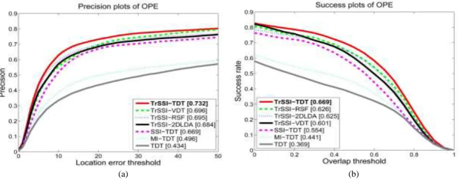
Fig. 4. The precision plots and the success plots of TrSSI-TDT, TrSSI-2DLDA, TrSSI-VDT, TDT, MI-TDT, SSI-TDT, and TrSSI-RSF on all the sequences: each decimal number in the legend is the representative precision or the representative success rate of the corresponding tracker: (a) the precision plots and (b) the success plots.
The transfer-learning-based semi-supervised improvement (TrSSI), semi-supervised improvement (SSI), and margin improvement (MI) enhance TDT, and the enhancement from SSI is higher than from MI. This indicates that TrSSI and SSI effectively adjust the graph embedding subspace.
Our TrSSI-TDT obtains more accurate results than TrSSI-2DLDA. This illustrates the effectiveness of the graph embedding for a discriminative representation for 2D tensors.
TrSSI-TDT yields more accurate results than TrSSI-VDT. As shown in the sixth and seventh examples in Fig. 3, when occlusion occurs, TrSSI-TDT still successfully tracks the objects, but TrSSI-VDT loses the track. This indicates that the 2-order tensor (image-as-matrix) representation which uses the projections U and V retains more useful structure information than image-as-vector representation which uses one projection.
TrSSI-TDT yields more accurate results than SSI-TDT. This indicates that historical information is effectively transferred into our object appearance model. This ensures that our tracker keeps the diversity of object appearance and avoids tracking drift after large changes in appearance, caused by large occlusions or serious pose or scale variations, etc.
TrSSI-TDT yields more accurate results than TrSSI-RSF. This indicates the effectiveness of the spatial filtering in our appearance model.
[image:23.595.58.520.113.293.2]The proposed transfer-learning-based semi-supervised improvement can be used for reference for other tracking algorithms for improving the tracking performance.
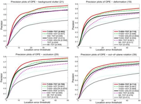
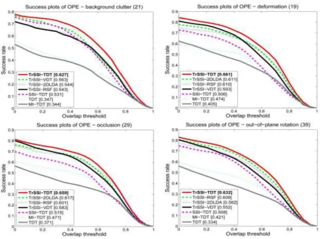
Fig. 5. The precision plots of TrSSI-TDT, TrSSI-2DLDA,TrSSI-VDT, TDT, MI-TDT, SSI-TDT, and TrSSI-RSF for different attributes.
Figs. 5 and 6 show, respectively, the precision plots and the success plots of TrSSI-TDT, TrSSI-2DLDA, TrSSI-VDT, TDT, MI-TDT, SSI-TDT, and TrSSI-RSF for annotated attributes, respectively. Due to the space limitation, only the plots for the attributes of occlusion, deformation, out-of-plane rotation, and background clutter are shown here. The plots for all the 11 annotated attributes are shown in the supplemental file which is published electronically. The following useful points are exhibited:
TrSSI always improves the tracking results except for low resolution videos. TDT and MI-TDT are not robust against large changes in illumination (such as in videos Car4, Cardark, Coke, David, and singer2), occlusions (such as in videos Coke, David3, and Lemming), and background clutter (such as in videos Football, Freeman4, and Lemming), etc. TrSSI-TDT can effectively handle large occlusions (such as in videos Coke, David3, Freeman4, and Lemming). However, the variants lose the track to some extent.
the results of SSI-TDT. For the videos with the attributes of background clutter, in-plane rotation, and illumination variation, transfer learning contributes as much as tensor representation and combination of transfer learning and tensor representation into the semi-supervised adjustment produces a large improvement in the results of our TrSSI-TDT.
Fig. 6. The success plots of TrSSI-TDT, TrSSI-2DLDA, TrSSI-VDT, TDT, MI-TDT, SSI-TDT, and TrSSI-RSF for different attributes.
5.2. Comparison with competing trackers
To show the effectiveness of TrSSI-TDT, we conducted a comparison between TrSSI-TDT and the 29 state-of-the-art trackers whose results were released on the CVPR 2013 benchmark dataset.
Fig. 7 shows some tracking results of TrSSI-TDT and the top 10 ranked competing trackers on the dataset. Fig. 8 shows the precision plots and the success plots of the top 10 ranked trackers among TrSSI-TDT and the 29 competing trackers on all the sequences in the benchmark dataset. The following useful points are seen: