On structural properties of the value function for an unbounded jump Markov process with an application to a processor sharing retrial queue

BIROn - Birkbeck Institutional Research Online

Bhulai, S. and Brooms, Anthony C. and Spieksma, F.M. (2014) On structural

properties of the value function for an unbounded jump Markov process with

an application to a processor sharing retrial queue. Queueing Systems 76

(4), pp. 425-446. ISSN 0257-0130.

Downloaded from:

Usage Guidelines:

Please refer to usage guidelines at

or alternatively

On structural properties of the value function for an

unbounded jump Markov process with an application to a

processor sharing retrial queue

S. Bhulai

_{, A.C. Brooms}

_{, and F.M. Spieksma}

Abstract

The derivation of structural properties for unbounded jump Markov processes cannot be done using standard mathematical tools, since the analysis is hindered due to the fact that the system is not uniformizable. We present a promising technique, a smoothed rate truncation method, to overcome the limitations of standard techniques and allow for the derivation of structural properties. We introduce this technique by application to a processor sharing queue with impatient customers that can retry if they renege. We are interested in structural properties of the value function of the system as a function of the arrival rate.

Keywords: monotonicity; processor-sharing queue; retrial queue; successive approximation.

1

Introduction

In practical applications of Markovian control problems, it is desirable that optimal strategies are well-behaved as a function of the input parameters of the problem. This facilitates computation or approximation of optimal policies. In order to check whether the model has such desirable properties, one needs the relative value function for average or discounted optimal costs to have structural properties such as monotonicity, convexity, and supermodularity (cf. [5]). A general method for checking such properties is the successive approximations method for discrete-time Markov decision chains.

When the original problem can be modeled as a continuous-time Markov decision process, application of the successive approximations method requires that the Markov decision process be uniformizable. In other words, the jump rates must be uniformly bounded as a function of action and state. In modern applications of Markov decision processes to call and contact center problems, however, the jump rates are generally unbounded functions of actions and states. Successive

∗_{VU University Amsterdam, Faculty of Sciences, De Boelelaan 1081a, 1081 HV Amsterdam, The Netherlands.}

†_{School of Economics, Mathematics & Statistics, Birkbeck College, Malet Street, Bloomsbury, London WC1E}

7HX, U.K.

approximations therefore is not applicable, even though the naive approach of simply applying the successive approximations operator without uniformization would preserve the required structural properties. No general method has been developed so far to attack this problem. Model-dependent techniques that have been used are, for instance, sample path based interchange arguments in a competing queues setting or finite state space truncation (see, e.g., [2]). The latter requires an ad hoc choice of the transitions on the boundary of the state space in order to keep the structure that is hidden in the original model, intact. It is not clear whether such an ad hoc choice can always be made.

We develop a novel method for attacking this problem and illustrate it by applying it to a processor sharing retrial queuing model. The proposed method is called the Smoothed Rate Truncation method (abbreviated: SRT, cf. Section 3). This method uses linearly smoothed transition rates, such that the smoothed system has a finite recurrent class, and such that it retains the structural properties of the infinite system. Linear smoothing has the advantage of destroying neither convexity nor concavity, provided the smoothing occurs already at low states. In other words, the rates that would take the system to a state with more customers in the system have to be smoothed in such a way that they become linear decreasing functions of the state variable. The SRT method seems to be a flexible method that we expect to be widely applicable. We then invoke a limiting argument to show that the relative value function for the non-smoothed model has the same desired structural properties as well. The limiting argument relies on continuity properties of a parametrized collection of Markov processes studied in [1] under the condition of uniform recurrence.

The paper is organized as follows. In the next section, we present the model to be studied. In Section 3 we set up the smoothed rate truncation method. In Section 4 we apply the smoothed rate truncation method to a processor sharing retrial queue.

2

Model description

Consider a service facilityQ1at which customers arrive according to a Poisson process with rateλ.

Customers at facilityQ1 are served according to a processor sharing discipline in which potential

inter-departure times are i.i.d. exponential with mean 1/µ. However, customers are impatient in the sense that they renege after an exponentially distributed period with mean 1/βindependently of all other customers in Q1, whilst waiting to complete service. A customer that reneges will

either abandon the system with probability 1−ψ or go to a retrial queueQ2 with probabilityψ.

Each customer in the retrial queue independently attempts to rejoin the tail of facilityQ1after an

exponentially distributed period with mean 1/γ. The retrial node will be modeled by a·/M/∞

queue. The inter-arrival times, potential inter-departure times, times spent inQ1before reneging,

times spent inQ2before retrial, and random variables governing exits immediately after reneging

constitute mutually independent sequences.

the customer joins facilityQ1with probability s, and balks with probability 1−s, independently

of all other customers. Note that this is equivalent to studying a system in which the arrival rate is bounded in interval (0, λ). In the sequel we will explicitly index all variables bysto denote this dependence on the joining rule.

We can model the system in a Markov theoretic framework. For this purpose, let (X(s), Y(s)) =

{Xt(s), Yt(s)}t≥0 be the Markov process associated with the number of customers in facilitiesQ1

andQ2, for joining rules, LetX =N0×N0denote the state space of the system, in other words,

(Xt(s), Yt(s)) = (x, y)∈ X, if at time t there are xcustomers in facility Q1 and y customers in

the retrial queueQ2.

We denote the corresponding transition rate from (x, y) to (x′_{, y}′_{) by q}

xy,x′y′(s). Then for

(x, y),(x′_{, y}′_{)6= (x, y)∈}

N0×N0we have

qxy,x′y′(s) =                   

λs, if (x′_{, y}′_{) = (x+ 1, y)}

µ1{x>0}+βx(1−ψ), if (x

′_{, y}′_{) = (x−1, y)}

βxψ, if (x′_{, y}′_{) = (x−1, y+ 1)}

γy, if (x′_{, y}′_{) = (x+ 1, y−1)}

0, otherwise

corresponding to arrivals, service departures and reneging customers that abandon, reneging cus-tomers that go to the retrial queue, and cuscus-tomers leaving the retrial queue, respectively.

For each s, (X(s), Y(s)) is an irreducible, non-explosive, conservative, standard Markov pro-cess. We assume that it has right-continuous paths. The associated transition function is denoted by the matrix function Pt(s) = Pt,x,y(s)_x,y. Due to abandonments, it is an ergodic Markov

process with stationary distributionπ(s), say, withπxy(s) denoting the stationary probability of

state (x, y), provided thatψ <1 orψ= 1 andλ < µ(cf. Lemma 3.2).

We assume that the system is subject to linear rate costs in each state (x, y), given by

d(x, y) =d1x+d2y,

for some constantsd1≥0 andd2≥0, independent ofs. As has been mentioned in the introduction,

the standard way of obtaining monotonicity properties is to uniformize the system and then apply a successive approximation scheme based on the Poisson equation for the relative value function

Vs. Define gs = π(s)d = P_(x,y)πxy(s)d(x, y) the expected average cost under the stationary

distributionπ(s) associated with joining rule s. Then,

Vs(x, y) = Z ∞

0

Pt,x,y(s)d(x, y)−gsdt.

The desired monotonicity and convexity properties then follow from monotonicity and convexity properties of the relative value function, given a fixed joining rule s.

Vsas a function ofs, properties of the finite horizon value function do not necessarily carry over

to the propertiesVs, since the constant being subtracted, gs, is a function ofs.

Before proceeding, let us first specify and define the structural properties that we are interested in. Letf :N0×N07→R. Thenf is

• Convex(x) iff(x+ 1, y)−f(x, y)≥f(x, y)−f(x−1, y) forx, y∈N0,x≥1;

• Convex(y)iff(x, y+ 1)−f(x, y)≥f(x, y)−f(x, y−1) forx, y ∈N0,y≥1;

• Supermodular(x,y) iff(x+ 1, y+ 1) +f(x, y)≥f(x, y+ 1) +f(x+ 1, y) forx, y ∈N0.

We are also interested in structural properties of the relative value function as a function ofs. Letf : [0,1]×N0×N07→R. Thenf is

• Convex(s) iff(s+ ∆, x, y)−f(s, x, y)≥f(s, x, y)−f(s−∆, x, y) forx, y∈N0;

• Supermodular(s,x)iff(s+∆, x+1, y)+f(s, x, y)≥f(s+∆, x, y)+f(s, x+1, y) forx, y∈N0;

• Supermodular(s,y)iff(s+∆, x, y+1)+f(s, x, y)≥f(s+∆, x, y)+f(s, x, y+1) forx, y∈N0.

Our main theorem is the following. Assume thatψ <1 or thatψ= 1 and λ < µ.

Theorem 2.1:

1. Vsis non-decreasing inxandy. Additionally, it is Convex(x), Convex(y), and Supermodular(x, y)

for eachs;

2. Vsis Supermodular(s, x), and Supermodular(s, y).

This theorem has the following consequences.

Corollary 2.2: gsis monotone non-decreasing and convex ins.

3

Smoothed Rate Truncation Method

In this section we introduce a novel truncation method. As we have discussed in the introduction, in general, finite state truncations that preserve the jump structure imply that the rates become concave as a function of state. This conflicts when one want to show convexity results for the relative value function.

To resolve this problem, we introduce a smoothed rate truncation method. The main idea in this method is to approximate the Markov decision process by (essentially) finite state Markov decision chains. This approximating Markov decision chain is obtained bylinearly decreasingthe relevant transition rates withincreasing state variableuntil these rates equal zero, hence the name

In our processor sharing retrial queue, the smoothed rate truncation method yields a pa-rameterized collection of approximating Markov chains. For each N let b(N) be such that limN→∞b(N) = ∞. Set A = {a = (u, s)|u ∈ {0} ∪ {1/N}N=1,...}. Clearly A is a compact

set in the topology inherited fromR

2_{. We define a parametrized collection (X(a), Y(a)),a∈}

Aby

specifying their rate matrix. Fora= (0, s) we takeQ(0, s) to be the rate matrix defined earlier. In other words (X(0, s), Y(0, s)) is the original processor sharing retrial queue with joining rules.

Fora= (1/N, s), put l=λs/N, k=γ/N,p=ψβ/b(N) and let for (x, y)∈ X

λNx,y(s) = max{0, λs−xl}; γN

x,y = max{0, γ−xk};

(βψ)Nx,y = max{0, ψβ−yp}.

The rate matrixQ(1/N, s) of the process (X(1/N, s), Y(1/N, s)) is defined by

qxy,x′y′(1/N, s) = λN_x,y(s)·1{(x+1,y)}(x

′_{, y}′_{) +γ}N

x,yy·1{(x+1,y−1)}(x

′_{, y}′₎

+(βψ)Nx,yx·1{(x−1,y+1)}(x

′_{, y}′₎

+(µ+β(1−ψ)x)·1{(x−1,y)}(x

′_{, y}′₎

1{1,...,N}(x)1{0,...,b(N)}(y)

+ξ1{(x,y−1)}(x

′_{, y}′_)·max{

1{N+1,...}(x),1{b(N)+1,...}(y)},

for (x′_{, y}′_{)6= (x, y), whereξwill be chosen later on. The ratesq}

xy,xy(1/N, s) make the row sums

ofQ(1/N, s) equal to 0.

These down ratesξare chosen so as to ensure that there is one closed class, and that this class is reached with probability 1 from any state outside the class. The irreducible class of states in the chain is precisely the set{(x, y)∈ X |x≤N, y≤b(N)}, and so essentially this is a finite state Markov chain. Note that we only smooth the rates that increase one of the components of the state variable.

The smoothing used here suffices for showing the desired convexity and supermodularity of the value function given a fixed joining rules. However, for studying the same properties of the value function as a function of the joining rule, we need to refine the smoothing (cf. Section 4).

This method can only work when the relevant performance measures of the Markov decision process can be approximated by the corresponding performance measures of smoothed truncated Markov decision chains. We will recall the results [1] guaranteeing the validity of such approach.

To this end, let us consider a collection of parametrized countable state Markov processes,

X(a) ={Xt(a)}t, where ais a parameter from a compact parameter setA. We assume that each

process is minimal and conservative with rate matrix Q(a). Moreover, each process X(a) has at most one closed class, plus possibly inessential states.

The functionf :E→R+is said to be amoment functionif there exists an increasing sequence

of finite setsEn↑E,n→ ∞, such that inf{f(x)|x6∈En} → ∞asn→ ∞. The following theorem

Theorem 3.1: We assume the following conditions to hold.

(i) {X(a)}a∈A isf-exponentially recurrent for a moment functionf. In other words, there exists

a moment functionf :E→R+, constantsc, d >0, and a finite setKwith X

qxz(a)f(z)≤ −cf(x) +d1{K}(x), x∈E, a∈A. (1)

(ii) There exists a function g:E→R+ and a constantc

′ _{such that}

X

qxz(a)g(z)≤c′g(x), x∈E, a∈A, (2)

with the property that there exists an increasing sequence of finite sets En ↑ E, such that

infx6∈Eng(x)/f(x)→ ∞as n→ ∞.

(iii) Continuity: a7→qxz(a),a7→Pzqxz(a)f(z) are continuous functions for eachx, z∈E.

Then the following properties hold.

(1) {X(a)}a isf-exponentially ergodic, i.e., there exist constants α, κ >0 such that X

z

|Pt,xz(a)−π(a)|f(z)≤κe−αtf(x), t≥0, a∈A,

where π(a) = (πx(a))x∈X is the unique stationary distribution ofX(a).

(2) Letc(a) = (c(x, a))x∈E,a∈A, be a cost function witha7→c(x, a) continuous for eachx∈E.

If supx|supac(x, a)|/f(x) < ∞, thena 7→ g(a) =π(a)c(a) = P

xπx(a)c(x, a) continuous

anda7→V(a) =R∞

0 Pt(a)(c(a)−g(a))dtis componentwise continuous.

f-exponential recurrence is well-studied in the literature. For instance, in [4] f-exponential recurrence and f-exponential ergodicity are shown to be equivalent in the case of one Markov process (#A = 1, i.e., the cardinality of the set A is one). If the parameter space is such that

{Q(a)}a∈Ahas the product property,f-exponential recurrence together withf-exponential

ergod-icity are used for studying average cost and discounted cost optimal strategies in a Markov decision process (cf. [3]; see also [1] for a discussion concerning the relation between these properties).

We will next show that our parametrized collection isf-exponentially recurrent for a function

f that grows exponentially in the state variable, provided that eitherψ <1 orψ= 1 andλ < µ. In caseψ= 1 andλ≥µ, the retrial queue is not positive recurrent, and so this case is not of our interest.

Lemma 3.2: (X(0,1), Y(0,1)) is not positive recurrent wheneverψ= 1 andλ≥µ.

Theorem 3.3: Suppose that eitherψ <1 orψ= 1 andλ < µ. Then there existǫ >0 andξ >0, such that the above defined parametrized collection of Markov processes (X(a), Y(a)), a∈A, is

f-exponentially recurrent for the functionf :E→R+ given by

f(x, y) = exp{ǫx+θǫy}, (3)

provided thatθ∈(1, ψ−1_{),b(N)≤N ψβ/γ, ifψ <1, andθ= 1 ifψ= 1 andλ < µ.}

Additionally, for each choice ofǫandθ satisfying the above restrictions, there existǫ′ > ǫand a constantc′ _{such that the function g:E→}

R+defined by

g(x, y) = exp{ǫ′_x+θǫ′_{y}, (4)}

satisfiesP

yqxy,x′y′(a)g(x′, y′)≤c′g(x, y),a∈A, (x, y)∈E.

In particular, conditions (i,ii, iii) of Theorem 3.1 are satisfied.

Proof : Continuity ofa 7→ qxy,x′_y′(a) holds by construction. Since the jump sizes are bounded

this impliesa7→P

x′y′qxy,x′y′(a)f(x′, y′).

It therefore suffices to show that there exist ǫ >0, a finite setK, and positive constantsc, d, such thatQ(u, s),u= 0,1/N,N = 1, . . ., satisfies (1) for the functionf from (3). In other words, we need to show the existence ofǫ >0, a finite setK and a constantc >0, such that

X

x′,y′

qxy,x′_y′(u, s)f(x′, y′)/f(x, y)≤ −c, (x, y)6∈K. (5)

Foru= 0, this reduces to findingǫ >0, a finite setK and a constantc >0, such that

λs(eǫ−1) +γy(eǫ−θǫ−1)1{y>0}

+βψx(e−ǫ+θǫ−1)1{x>0}+ (µ+β(1−ψ)x)(e

−ǫ₋₁₎

1{x>0}≤ −c, (x, y)6∈K. (6)

Rewriting yields

λs(eǫ_{−1) +γy(e}ǫ−θǫ₋₁₎

1{y>0}

+µ(e−ǫ−1)1{x>0}+βx ψe

−ǫ_(eθǫ_{−1) + (e}−ǫ₋₁₎

1{x>0}≤ −c. (7)

First we assume that ψ <1. If the coefficients of bothxandy in the above expression are both negative, then clearly a finite set K and constant c can be found for (7). The coefficient ofy is negative providedθ >1. The coefficient ofxequals 0 ifǫ= 0. The derivative toǫatǫ= 0 equals

θψ−1,

which is negative if θ < 1/ψ. This settles the case for all Markov processes (X(0, s), Y(0, s)). Next we turn to the smooth approximations (X(1/N, s), Y(1/N, s)). To this end we compute the difference of the resulting expression and the left-hand side of (6). This yields for 0≤x≤N,0≤

y≤b(N)

A sufficient condition for this to be non-negative is

k(eǫ−θǫ−1) +p(e−ǫ+θǫ−1)≥0. (8)

By a similar reasoning as before, we find that the derivative of the left-hand side above is non-negative atǫ= 0 if

k(1−θ) +p(θ−1)≥0.

In other words, ifp≥k, or

ψβ b(N) ≥

γ N,

that isN ≥γb(N)/ψβ.

Ifx > N and/or y > b(N), then it is easily checked that one can choose ξ large enough so that (5) holds for these values of xand y and all parameters. It is easily checked that ǫ can be increased without violating (7) and (8). This yields existence of the function g with the desired properties.

In case thatψ= 1 andλ < µwe take θ= 1. The rest is standard (cf. [4]).

Corollary 3.4: ForV(a) the value function associated with (X(a), Y(a)), we have that

V(1/N, s)→V(0, s), N → ∞,

componentwise.

Note: The constructed parametrized models are all stochastically monotonic (cf. [7]). As in [7] one can construct a function ˆf for which this collection is ˆf-exponentially recurrent with set

K={0}. The results in [7] then imply that the ˆf-exponential ergodicity property holds with rate constantα=c. In other words, we can explicitly compute a bound on the rate of convergence to stationarity. This means that

sup

x,y

1 ˆ

f(x, y)

Vx,y(a)− Z T

0

Ex,yd(Xt(a), Yt(a))−Eπ(a)d(Xt(a), Yt(a))

dt ≤K

e−cT c ,

and so it suffices to approximate the total expected cost over a finite time interval to get an approximation of the relative value function.

The following step to prove is thatV1/N,s have the desired structural properties. This will be

the subject of the next section.

4

Structural results for processor sharing retrial queue

For each N fixed, the associated smoothed rate truncation (X(1/N, s), Y(/N, s)) has the closed recurrent class of states

It is sufficient to restrict the state space toXN_.

In this section we will provide the proof of Theorem 2.1 by using value iteration applied to approximating processes. For the proof of the first part we can use the approximations discussed in the previous section. The proof of the second part concerning the behavior of the value function as a function of the joining rule requires a more refined approximation technique. This will be discussed later on.

First we prove the following theorem.

Theorem 4.1: V1/N,s is non-decreasing in xand y, and, ifkN :=γ/N =ψβ/b(N) =:pN, it is

Convex(x), Convex(y) and Supermodular(x, y) onXN_{, for anyN ≥1.}

We will show that Theorem 4.1 implies the validity of the first part of Theorem 2.1.

Proof of Theorem 2.1 (1): : Theorem 4.1 requires that kN =pN for Convex(x), Convex(y)

and

Supermodular(x, y) to hold. In turn, this requires thatb(N) =N ψβ/γ be integer for at least an infinite sequence of values ofN. To solve this, we slightly perturbγ.

To this end, put b(N) = ⌊N ψβ/γ⌋. Then kN = γ/N < pN = ψβ/b(N). Next choose the

perturbed parameterγ(N) =N pN. Then

γ < γ(N)≤γ· ψβ

ψβ−(γ/N).

Moreover,γ(N)/N=ψβ/b(N), so that the condition of Theorem 4.1 is satisfied.

Consider the parametrized collection ( ˆX(u, s),Yˆ(u, s)),u∈ {0}∪{1/N}N≥N0, where ˆX(0, s) =

X(0, s), ˆY(0, s) =Y(0, s), and ( ˆX(1/N, s),Yˆ(1/N, s)) is the SRT, with rateγ(N) instead ofγ, and closed set of statesXN _{withb(N) specified as above. By inspection of the proof of Theorem 3.3,}

it follows that this collection satisfies the conditions of Theorem 3.1. The result follows directly taking the limitN → ∞.

For the proof of Theorem 4.1 we fix N. We will use a standard successive approxima-tions argument, applied to the uniformized chain with uniformization constant η = λ+µ+

βb(N) +γN. One then applies successive approximations to the discrete time chain, denoted by (Xd_{(1/N, s), Y}d_{(1/N, s)) with transition probabilities}

Pxy,x′_y′(1/N, s) =δ_xy,x′_y′ +

1

ηqxy,x′y′(1/N, s), (x, y),(x

′_{, y}′_{)∈ X}N_.

Scaling the cost rates also byη, the relative value function for the associated discrete time model equals the continuous relative value function (cf. Lippman [6], Serfozo [9]). Now, rescaling the rates by a factorηand denoting these again bys,β,γandµ, we have to slightly modify the cost function

dη(x, y) =d1x+d2y

η .

LetV0

s ≡0 onXN. The successive approximations scheme applied to discrete time

approxi-mation yields

Vsn+1(x, y) = λNx,y(s)Vsn(x+ 1, y) +1{x>0}µV

n

s(x−1, y) +1{y>0}γ

N

x,yVsn(x+ 1, y−1)

+1{x>0}βx(1−ψ)V

n

s (x−1, y) +1{x>0}(βψ)

N

x,yxVsn(x−1, y+ 1)

+(1−λNxy(s)−µ1{x>0}−(β−yp)x−γ

N

xyy)Vsn(x, y) + (d1x+d2y),

where Vn

s (x′, y′) = 0 for (x′, y′) 6∈ XN. By virtue of (Lippman [6], Serfozo [9]), Vsn(x, y)− Vn

s(0,0)→V1/N,s(x, y)−V1/N,s(0,0), asn→ ∞.

For proving the induction step, a general principle is to take out the smallest common factor in front of difference terms, or the factor in front of the largest term.

Theorem 4.2: Vn

1/N,sand the relative value functionV1/N,sare non-decreasing function in both

variablesx, y onXN_.

Proof : Here, as in the proofs of the next theorems, we suppress the dependence on the parameter

N in our notation. Since V0

s ≡ 0, this function is clearly non-decreasing in both x and y. Therefore, assume

that Vn

s is non-decreasing in xand y. We first show that Vsn+1 is non-decreasing in x. To this

end, define Vn

s (x, y) = Vsn(0, y) for x <0 and Vsn(x, y) = Vsn(x,0) for y < 0. Then, consider

0≤x < N −1 and 0≤y < b(N). Then,

Vsn+1(x+ 1, y)−Vsn+1(x, y) =d1[(x+ 1)−x]

+(λs−(x+ 1)l)Vsn(x+ 2, y)−(λs−xl)Vsn(x+ 1, y)

+µ[Vsn(x, y)−Vsn(x−1, y)]

+(γ−(x+ 1)k)y Vsn(x+ 2, y−1)−(γ−xk)y Vsn(x+ 1, y−1)

+(x+ 1)β(1−ψ)Vn

s (x, y)−xβ(1−ψ)Vsn(x−1, y)

+(x+ 1)(βψ−yp)Vsn(x, y+ 1)−x(βψ−yp)Vsn(x−1, y+ 1)

+(1−(λs−(x+ 1)l)−µ−(β−yp)(x+ 1)−(γ−(x+ 1)k)y)Vsn(x+ 1, y)

−(1−(λs−xl)−µ−(β−yp)x−(γ−xk)y)Vsn(x, y)

≥ (λs−(x+ 1)l) [Vsn(x+ 2, y)−Vsn(x+ 1, y)]

+(γ−(x+ 1)k)y[Vn

s (x+ 2, y−1)−Vsn(x+ 1, y−1)]

+βx(1−ψ) [Vsn(x, y)−Vsn(x−1, y)] +β(1−ψ)Vsn(x, y)

+x(βψ−yp) [Vsn(x, y+ 1)−Vsn(x−1, y+ 1)] + (βψ−yp)Vsn(x, y+ 1)

+(1−(λs−xl)−µ−(β−yp)(x+ 1)−y(γ−xk)) [Vsn(x+ 1, y)−Vsn(x, y)]

−(β−yp)Vsn(x, y)

≥ d1+ (βψ−yp) [Vsn(x, y+ 1)−Vsn(x, y)]

For the first inequality we interchange the terms (λs−xl)Vn

s(x+1, y) and (λs−(x+1)l)Vsn(x+1, y);

we use non-decreasingness inx, y for the first and second inequalities.

At the boundary x=N−1 andy =b(N) the induction step follows in the same way as the above, since naturally the transition rates leading outside XN _{are 0 and so one may defineV}n s

outsideXN _{as one likes.}

We now continue the proof by showing that Vsn+1 is increasing in y. To this end, consider

0≤x < N and 0≤y < b(N)−1. Then,

Vsn+1(x, y+ 1)−Vsn+1(x, y)

= d2[(y+ 1)−y] + (λs−xl)[Vsn(x+ 1, y+ 1)−Vsn(x+ 1, y)]

+µ[Vsn(x−1, y+ 1)−Vsn(x−1, y)]

+βx(1−ψ)Vsn(x−1, y+ 1)−βx(1−ψ)Vsn(x−1, y)

+x(βψ−(y+ 1)p)Vsn(x−1, y+ 2)−x(βψ−yp)Vsn(x−1, y+ 1)

+(y+ 1)(γ−xk)Vsn(x+ 1, y)−y(γ−xk)Vsn(x+ 1, y−1)

+(1−(λs−xl)−µ−(β−(y+ 1)p)x−(y+ 1)(γ−xk))Vn

s(x, y+ 1)

−(1−(λs−xl)−µ−(β−yp)x−y(γ−xk))Vsn(x, y)

≥ y(γ−xk) [Vsn(x+ 1, y)−Vsn(x+ 1, y−1)] + (γ−xk) (Vsn(x+ 1, y)−Vs(x, y)

+px(Vsn(x, y+ 1)−Vsn(x−1, y+ 1))

+(1−(λs−xl)−µ−(β−yp)x−(y+ 1)(γ−xk) [Vsn(x, y+ 1)−Vsn(x, y)]

≥ (γ−xk) [Vsn(x+ 1, y)−Vsn(x, y)] +px(Vsn(x, y+ 1)−Vsn(x−1, y+ 1))

≥ 0.

Both inequalities follows from the induction hypothesis by using increasingness inxand y. The last inequality uses increasingness in x, y. One can easily check that in a similar way the result also holds for the boundaries corresponding to x = N and y = b(N)−1. The proof is finally concluded by taking the limit asn→ ∞.

Let us now move on to second-order properties ofV1/N,s.

Theorem 4.3: Vn

1/N,s, V1/N,s are Convex(x), Convex(y) and Supermodular(x, y) onX N_{, ifk}

N = γ/N =pN =ψβ/b(N).

Proof : V0

s ≡0 has the three properties Convex(x), Convex(y), and Supermodular(x,y). Assume

that these properties hold forVn

s . We first show thatVsn+1satisfies Convex(x). To this end, define Vn

and 0≤y < b(N). Then,

Vsn+1(x+ 1, y)−2Vsn+1(x, y) +Vsn+1(x−1, y)

= (λs−(x+ 1)l)Vsn(x+ 2, y)−2(λs−xl)Vsn(x+ 1, y) + (λs−(x−1)l)Vsn(x, y)

+µ[Vsn(x, y)−2Vsn(x−1, y) +Vsn(x−2, y)]

+β(1−ψ) [(x+ 1)Vn

s (x, y)−2x Vsn(x−1, y) + (x−1)Vsn(x−2, y)]

+(βψ−yp) [(x+ 1)Vsn(x, y+ 1)−2x Vsn(x−1, y+ 1) + (x−1)Vsn(x−2, y+ 1)]

+(γ−(x+ 1)k)yVsn(x+ 2, y−1)−2(γ−xk)yVsn(x+ 1, y−1)

+(γ−(x−1)k)yVsn(x, y−1)

+(1−(λs−(x+ 1)l)−µ−(β−yp)(x+ 1)−y(γ−(x+ 1)k))Vsn(x+ 1, y)

−2(1−(λs−xl)−µ−(β−yp)x−y(γ−xk))Vn s(x, y)

+(1−(λs−(x−1)l)−µ−(β−yp)(x−1)−y(γ−(x−1)k)Vsn(x−1, y)

≥ (λs−(x+ 1)l)[Vsn(x+ 2, y)−2Vsn(x+ 1, y) +Vsn(x, y)]

+2l[Vsn(x, y)−Vsn(x+ 1, y)]

+β(1−ψ)(x−1)[Vsn(x, y)−2Vsn(x−1, y) +Vsn(x−2, y)]

+2β(1−ψ) [Vsn(x, y)−Vsn(x−1, y)]

+(βψ−yp)(x−1)[Vn

s (x, y+ 1)−2Vsn(x−1, y+ 1) +Vsn(x−2, y+ 1]

+2(βψ−yp) [Vsn(x, y+ 1)−Vsn(x−1, y+ 1)]

+(γ−(x+ 1)k)y[Vsn(x+ 2, y−1)−2Vsn(x+ 1, y−1) +Vsn(x, y−1)]

+2ky[Vsn(x, y−1)−Vsn(x+ 1, y−1)]

+(1−(λs−(x−1)l)−µ−(β−yp)(x+ 1)

−y(γ−(x−1)k))[Vn

s (x+ 1, y)−2Vsn(x, y) +Vsn(x−1, y)]

+2l[Vsn(x+ 1, y)−Vsn(x, y)]−2(β−yp)[Vsn(x, y)−Vsn(x−1, y)]

+2ky[Vsn(x+ 1, y)−Vsn(x, y)]

≥ 0.

The first inequality follows from the induction hypothesis on the terms having the factor µ. In the second inequality the terms with factor 2lcancel; we use Supermodular(x−1, y) for the terms with factor 2(βψ−yp), so that the terms with factor 2β all cancel; we use Supermodular(x, y−1) for the terms with factor 2ky; for the remaining terms evidently one should use the appropriate convexity properties.

As before the boundaries x=N −1 and y =b(N) follow in the same manner, by the usual argument that the rates leading out ofXN _{are zero.}

Then

Vsn+1(x, y+ 1)−2Vsn+1(x, y) +Vsn+1(x, y−1)

≥ µ[Vsn(x−1, y+ 1)−2Vsn(x−1, y) +Vsn(x−1, y−1)]

+x[(βψ−(y+ 1)p)Vsn(x−1, y+ 2)−2(βψ−yp)Vsn(x−1, y+ 1)

+(βψ−(y−1)p)Vn

s(x−1, y)]

+β(1−ψ)x[Vsn(x−1, y+ 1)−2Vsn(x−1, y) +Vsn(x−1, y−1)]

+(γ−xk) [(y+ 1)Vsn(x+ 1, y)−2y Vsn(x+ 1, y−1) + (y−1)Vsn(x+ 1, y−2)]

+(1−(λs−xl)−µ−(β−(y+ 1)p)x−(y+ 1)(γ−xk))Vsn(x, y+ 1)

−2(1−(λs−xl)−µ−(β−yp)x−y(γ−xk))Vsn(x, y)

+(1−(λs−xl)−µ−(β−(y−1)p)x−(y−1)(γ−xk))Vsn(x, y−1)

≥ x(βψ−(y+ 1)p)[Vsn(x−1, y+ 2)−2Vsn(x−1, y+ 1) +Vsn(x−1, y)]

+2(γ−xk) [Vsn(x+ 1, y)−Vsn(x+ 1, y−1)−Vsn(x, y) +Vsn(x, y−1)]

+(1−(λs−xl)−µ−(β−(y−1)p)x

−(y+ 1)(γ−xk))[Vsn(x, y+ 1)−2Vsn(x, y) +Vsn(x, y−1)]

≥ 0.

The first inequality follows from Convex(y) for the term with (λs−xl). The second from Convex(y) for the terms withµandβ(1−ψ)x; from Convex(y−1) for the term withγ−xk, and by rearranging terms such that Supermodular (x−1, y) parts of the induction hypothesis can be used. The second inequality follows from Convex(y), Convex(y+ 1) and Supermodular(x, y−1). The result also holds trivially at the boundariesx=N andy=b(N)−1 by the same arguments as before.

b(N)−1. Then

Vsn+1(x+ 1, y+ 1) +Vsn+1(x, y)−Vsn+1(x+ 1, y)−Vsn+1(x, y+ 1)

= (λs−(x+ 1)l)Vsn(x+ 2, y+ 1) + (λs−xl)Vsn(x+ 1, y)

−(λs−(x+ 1)l)Vsn(x+ 2, y)−(λs−xl)Vsn(x+ 1, y+ 1)

+µ[Vn

s(x, y+ 1) +Vsn(x−1, y)−Vsn(x, y)−Vsn(x−1, y+ 1)]

+β(1−ψ) (x+ 1)Vsn(x, y+ 1) +β(1−ψ)x Vsn(x−1, y)

−β(1−ψ)(x+ 1)Vsn(x, y)−β(1−ψ)x Vsn(x−1, y+ 1)]

+(βψ−(y+ 1)p) (x+ 1)Vsn(x, y+ 2) + (βψ−yp)x Vsn(x−1, y+ 1)

−(βψ−yp)(x+ 1)Vsn(x, y+ 1)−(βψ−(y+ 1)p)x Vsn(x−1, y+ 2)]

+(γ−(x+ 1)k) (y+ 1)Vn

s(x+ 2, y)

+(γ−xk)y Vsn(x+ 1, y−1)−(γ−(x+ 1)k)y Vsn(x+ 2, y−1)

−(γ−xk) (y+ 1)Vsn(x+ 1, y)

+(1−(λs−(x+ 1)l)−µ−(β−(y+ 1)p)(x+ 1)−(y+ 1)(γ−(x+ 1)k))Vsn(x+ 1, y+ 1)

+(1−(λs−xl)−µ−(β−yp)x−y(γ−xk))Vsn(x, y)

−(1−(λs−(x+ 1)l)−µ−(β−yp)(x+ 1)−y(γ−(x+ 1)k))Vn

s(x+ 1, y)

−(1−(λs−xl)−µ−(β−(y+ 1)p)x−(y+ 1)(γ−xk))Vsn(x, y+ 1)

≥ (λs−(x+ 1)l)[Vsn(x+ 2, y+ 1) +Vsn(x+ 1, y)−Vsn(x+ 2, y)−Vsn(x+ 1, y+ 1)]

+β(1−ψ)x[Vsn(x, y+ 1) +Vsn(x−1, y)−Vsn(x, y)−Vsn(x−1, y+ 1)]

+(βψ−(y+ 1)p)x[Vsn(x, y+ 2) +Vsn(x−1, y+ 1)−Vsn(x, y+ 1)−Vsn(x−1, y+ 2)]

+β(1−ψ)[Vsn(x, y+ 1)−Vs(x, y)] + (βψ−(y+ 1)p)[Vsn(x, y+ 2)−Vsn(x, y+ 1)]

+pxVn

s(x−1, y+ 1)−p(x+ 1)Vsn(x, y+ 1)

+(γ−(x+ 1)k)y[Vsn(x+ 2, y) +Vsn(x+ 1, y−1)−Vsn(x+ 2, y−1)−Vsn(x+ 1, y)]

(γ−(x+ 1)k)Vsn(x+ 2, y) +kyVsn(x+ 1, y−1)−k(y+ 1)Vsn(x+ 1, y)

−(γ−(x+ 1)k)Vsn(x+ 1, y)

+(1−(λs−xl)−µ−(β−yp)(x+ 1)−(y+ 1)(γ−xk))[Vsn(x+ 1, y+ 1) +Vsn(x, y)

−Vn

s(x+ 1, y)−Vsn(x, y+ 1)]

+p(x+ 1)Vsn(x+ 1, y+ 1) + (β−yp)Vsn(x, y)−pxVsn(x, y+ 1)−(β−yp)Vsn(x, y+ 1)

+k(y+ 1)Vn

s (x+ 1, y+ 1) + (γ−xk)Vsn(x, y)−(γ−(x+ 1)k)Vsn(x+ 1, y)

−k(y+ 1)Vsn(x+ 1, y)

≥ p(Vsn(x+ 1, y+ 1) +Vsn(x, y)−2Vsn(x, y+ 1)) +k(Vsn(x+ 1, y+ 1) +Vsn(x, y)−2Vsn(x+ 1, y))

≥ 0,

µ. The second inequality follows by rearranging terms such that the induction hypothesis can be used again. For the final inequality we use Supermodular(x, y). The result also holds for the boundaries. Finally, the proof is concluded by taking the limit asn→ ∞.

Proof of Theorem 4.1 : By combination of Theorems 4.2 and 4.3.

As has been mentioned in Section 2, structural properties of the value function as a function of the joining rules (or, equivalently, the arrival rateλ) are much harder to obtain by value iteration. Comparing systems with different joining rules, and smoothing as we did before, has the effect that the smoothed arrival rates for the system with the larger joining rule decreasefasterthan for the system with a smaller joining rule. This destroys propagation of the induction step.

A solution to this problem is by smoothing the arrivals for different joining rules at the same rate, independently of the γ-transfers. This solves the problem up to the x-boundary where the smoothed arrival rates for the approximation with a smaller initial joining rule becomes 0. For larger values of x we have the same problem that we indicated above. As in the previous analysis (where we used compensation ofγ-transitions byβψ-transitions or vice versa in showing supermodularity), this can be solved by introducing transitions in the opposite direction.

First fixs∈(0,1), and ∆, such thats+ ∆, s−∆∈[0,1]. Hence we restrict to the joining rules [s′_{], s}′_{∈ {s−∆, s, s+ ∆}. It is convenient to chooses,∆ such thatλs, ∆sare rational. Further,}

we choose a sequence{Nt}t⊂N0, such thatNt(s−∆)/(s+ ∆),Nt∆/(∆ +s) are integer. Further

we putlt=λ(s+ ∆)/Ntand putMt=λ(s−∆)/lt. By our conditionMt is integer.

Next we construct the processes (X(1/Nt, s′), Y(1/N, s′), s′ ∈ {s−∆, s, s+ ∆} in the same

way as in Section 4, except that we smooth the arrival rates differently. Forx≤Nt,y≤b(Nt)

λNt

x,y(s−∆) = max{λ(s−∆)−xlt,0}, λNt

x,y(s) = max{(λs−xlt) 0}, λNt

x,y(s−∆) = λ(s+ ∆)−xlt.

We further increase the departure rates by putting

µNt

x,y(s−∆) = µ+β(1−ψ)x+ltx, µNt

x,y(s+ ∆) =µN

t

s,x,y = µ+β(1−ψ)x+ min{ltx, Mtlt}.

The N-approximations (X(1/Nt, s′), Y(1/Nt, s′), s′ ∈ {s−∆, s, s+ ∆} live on the finite space

XNt. As in Theorem 3.3 it can be checked that the collection {X(1/N

t, s′), Y(1/Nt, s′), s′ ∈

Without loss of generality we may suppress the dependence ont in our notation. We index the corresponding finite horizon expected total cost functions in the same manner as before. It is straightforward to show that Vn

1/N,s′ is increasing in x and y on X

N_{, for n, N = 1, . . .,}

s′_{∈ {s−∆, s, s+ ∆}. Moreover,V}n

1/N,s−∆is Convex(x), Convex(y) and Supermodular(x, y). This

can be seen directly from the equations used for showing these properties for the approximations from Section 4. Note that a problem may only occur at the boundaryx=M. We will show the following theorem.

Theorem 4.4: V1/N,s′ is non-decreasing ins′∈ {s−∆, s, s+∆}, and, ifkN :=γ/N =ψβ/b(N) =: pN, it is Convex(s′) ons′ ∈ {s−∆, s, s+ ∆}and Supermodular(s′, x) on Supermodular(s′, y) on s′_{∈ {s−∆, s} ors}′_{∈ {s−∆, s+ ∆}, all onX}N_{, for any N≥1.}

Proof of Theorem 2.1 (2): : This is a copy of the proof of Theorem 2.1 (1).

Let us now proceed to proving Theorem 4.4. It consists of a number of steps.

Theorem 4.5: Vn

1/N,s′ is componentwise non-decreasing in s

′ _{∈ {s−∆, s, s+ ∆} on X}N_{, for} n= 1, . . ., , and so isV1/N,s′.

Proof : The statement clearly holds forV0

s′ ≡0. Assume hence that the statement is true upto

valuen.

Let first 0≤x≤M, 0≤y < b(N). Then,

Vn+1

s (x, y)−Vsn−+1∆(x, y)

= (λs−xl)Vsn(x+ 1, y)−(λ(s−∆)−xl)Vsn−∆(x+ 1, y)

+µ[Vsn(x−1, y)−Vsn−∆(x−1, y)] + (βx(1−ψ) +lx) [Vsn(x−1, y)−Vsn−∆(x−1, y)]

+x(βψ−yp) [Vsn(x−1, y+ 1)−Vsn−∆(x−1, y+ 1)]

+y(γ−xk) [Vsn(x+ 1, y−1)−Vsn−∆(x+ 1, y−1)]

+(1−(λs−xl)−µ−(β−yp)x−lx−y(γ−xk))Vn s (x, y)

−(1−(λ(s−∆)−xl)−µ−(β−yp)x−lx−y(γ−xk))Vsn−∆(x, y)

≥ (λ(s−∆)−xl) [Vn

s (x+ 1, y)−Vsn−∆(x+ 1, y)] +λ∆[Vsn(x+ 1, y)−Vsn(x, y)]

+(1−(λ(s−∆)−xl)−µ−(β−yp)x−lx−y(γ−xk)) [Vsn(x, y)−Vsn−∆(x, y)]

≥ λ∆[Vsn(x+ 1, y)−Vsn(x, y)]

≥ 0.

The first two inequalities follow from applying the induction hypothesis by using increasingness ins′_{. The last inequality follows from increasingness inx.}

Suppose that M < x ≤ N, y ≤ b(N). First suppose that λN

x,y(s) > 0. The only λ-terms

occurring are factors ofVn

s(x, y) andVsn(x+ 1, y). This is easily seen to give a contribution (λs− xl)[Vn

terms of factors withxl−M landM l, we get the extra term (xl−M l)[Vn

s−∆(x, y)−Vsn−∆(x−1, y)]

By increasingness inxofVn

s−∆, this contribution is non-negative.

The case of λN

x,y(s) = 0 is similar.

For the boundaries y=b(N) andx=N, the argument is precisely the same as in the above, since the rates leading out ofXN _{are 0.}

A similar derivation holds, when comparing Vsn andVsn+∆. The proof is concluded by taking

the limit asn→ ∞.

The extension of Theorem 4.3 to our adapted SRT provides the necessary ingredients for showing convexity in s′_{. Note that, similar to the case of the first-order properties, the proof of this}

result only depends on the properties of the facilityQ1, i.e., convexity inxin this case. However,

convexity in x depends on convexity in y for queue Q2. For the convexity in s′ we also need

supermodularity ins′ _{in combination with the other variables.}

Theorem 4.6: Vn

1/N,s′ is Convex(s

′_{) on{s−∆, s, s+∆}, andV}n

1/N,s′, V1/N,s′are Supermodular(s−

∆, x) and Supermodular(s−∆, y) on {s−∆, s}and{s−∆, s+ ∆}.

Proof : ForV0

s′(x, y)≡0, clearly this function satisfies Convex(s′) on{s−∆, s, s+ ∆}, as well as

Supermodular(s−∆, x) and Supermodular(s−∆, y) on{s−∆, s}and{s−∆, s+ ∆}. Therefore, assume that these properties hold forVn

s′. We first show thatV n+1

s′ satisfies Convex(s′). To this

end, consider 0≤x≤M and 0≤y < b(N). Then,

Vn_s+∆+1(x, y)−2Vn+1

s (x, y) +V n+1

s−∆(x, y)

≥(λ(s+ ∆)−xl)Vsn+∆(x+ 1, y)−2(λs−xl)Vsn(x+ 1, y) + (λ(s−∆)−xl)Vs−∆(x+ 1, y)

+ (1−(λ(s+ ∆)−xl)−µ−lx−(β−py)x−y(γ−xk))Vsn+∆(x, y)

−2(1−(λs−xl)s−µ−lx−(β−py)x−y(γ−xk))Vsn(x, y)

+ (1−(λ(s−∆)−xl)−µ−lx−(β−py)x−y(γ−xk))Vsn−∆(x, y)

≥2λ∆ [Vsn(x+ 1, y)−Vsn−∆(x+ 1, y)−Vsn(x, y) +Vsn−∆(x, y)]

≥0.

The first inequality follows from the induction hypothesis on the terms having factors with no

s. The second inequality follows by rearranging terms such that the induction hypothesis can be used again on terms with factorλ(s+ ∆)−xland 1−(λ(s+ ∆)−xl)−µ−lx−(β−py)x−yγ. The final inequality follows from Supermodular(s−∆, x) on{s−∆, s}.

Next consider the case M ≤x≤N, withλN

x,y(s)>0. Separating the departure rates xlinto

terms with factorM l=λ(s−∆) and with factorxl−M l=xl−λ(s−∆), we get

(λ(s+ ∆)−xl)Vsn+∆(x+ 1, y)−2(λs−xl)Vsn(x+ 1, y)

+(xl−M l)[Vsn−∆(x−1, y)−Vsn−∆(x, y)] +M l Vsn−∆(x, y)

−2(1−(λs−xl)s−µ−M l−(β−py)x−y(γ−xk))Vsn(x, y)

+(1−µ−M l−(β−py)x−y(γ−xk))Vsn−∆(x, y)

≥ (λ(s+ ∆)−xl)Vsn+∆(x+ 1, y)−2(λs−xl)Vsn(x+ 1, y)

+(xl−λ(s−∆))[Vsn−∆(x, y)−Vsn−∆(x+ 1, y)]

+(1−(λ(s+ ∆)−xl)−µ−M l−(β−py)x−y(γ−xk))Vsn+∆(x, y)

−2(1−(λs−xl)s−µ−M l−(β−py)x−y(γ−xk))Vsn(x, y)

+(1−µ−M l−(β−py)x−y(γ−xk))Vsn−∆(x, y),

where we have used thatVn

s−∆is Convex(x). The rest is analogous to the previous.

Finally, we consider the case that alsoλN

x,y(s) = 0. The only terms of interest to consider are

(λ(s+ ∆)−xl)[Vn

s+∆(x+ 1, y)−Vsn+∆(x, y)]−(xl−lM)[Vsn−∆(x, y)−Vsn−∆(x−1, y)],

which is non-negative by first applying Supermodular(s−∆, x) (w.r.t{s−∆, s+ ∆}) to the first term and then Convex(x) for Vsn−∆. Note that λ(s+ ∆) ≥ lM. The result also holds at the

boundaries corresponding tox=N and y=b(N).

We next proceed to prove Supermodular(s−∆, x) on{s−∆, s}. The proof on{s−∆, s+ ∆}is completely analogous. To this end, consider 0≤x < M and 0≤y < b(N).

Vsn+1(x+ 1, y) +Vsn−+1∆(x, y)−V

n+1

s (x, y)−Vsn−+1∆(x+ 1, y)

≥ (λs−(x+ 1)l)Vsn(x+ 2, y) + (λ(s−∆)−xl)Vsn−∆(x+ 1, y)

−(λs−xl)Vsn(x+ 1, y)−(λ(s−∆)−(x+ 1)l)Vsn−∆(x+ 2, y)

+(β(1−ψ) +l) [(x+ 1)Vsn(x, y) +x Vsn−∆(x−1, y)

−x Vsn(x−1, y)−(x+ 1)Vsn−∆(x, y)]

+(βψ−yp) [(x+ 1)Vn

s(x, y+ 1)

+x Vn

s−∆(x−1, y+ 1)−x Vsn(x−1, y+ 1)−(x+ 1)Vsn−∆(x, y+ 1)]

+(γ−(x+ 1)k)y Vsn(x+ 2, y−1) + (γ−xk)y Vsn−∆(x+ 1, y−1)

−(γ−xk)y Vsn(x+ 1, y−1)−(γ−(x+ 1)k)y Vsn−∆(x+ 2, y−1)

+(1−(λs−(x+ 1)l) −µ−(x+ 1)l−(β−yp)(x+ 1)−y(γ−(x+ 1)k))Vsn(x+ 1, y)

+(1−(λ(s−∆)−xl)−µ−xl−(β−yp)x−y(γ−xk))Vsn−∆(x, y)

−(1−(λs−xl)−µ−xl−(β−yp)x−y(γ−xk))Vsn(x, y)

−(1−(λ(s−∆)−(x+ 1)l)−µ−(x+ 1)l−(β−yp)(x+ 1)−y(γ−(x+ 1)k))Vsn−∆(x+ 1, y)

≥ ∆λ[Vsn−∆(x+ 2, y)−2Vsn−∆(x+ 1, y) +Vsn−∆(x, y)]

+l[Vn

s−∆(x+ 1, y)−Vsn(x+ 1, y) +Vsn(x+ 1, y)−Vsn−∆(x+ 1, y)]

+(β(1−ψ) +l) [Vsn(x, y)−Vsn−∆(x, y) +Vsn−∆(x, y)−Vsn(x, y)]

+(βψ−yp) [Vsn(x, y+ 1)−Vsn−∆(x, y+ 1) +Vsn−∆(x, y)−Vsn(x, y)]

≥ 0.

The first inequality follows from the induction hypothesis on terms having only the factor µ. The second inequality follows by rearranging terms such that the induction hypothesis can be used on terms with factors λs−(x+ 1)l, (β(1−ψ) +l)x, (βψ−yp)x, (γ−(x+ 1)k)y, and 1−(λs−xl)−µ−(x+ 1)l−(β−yp)(x+ 1)−y(γ−xk). The final inequality follows from Convex(x+ 1) (w.r.t. s−∆) for the first; and Supermodular(s−∆, y) and Supermodular(s−∆,

y−1) for the two last lines.

Suppose thatx≥M withλN_{(x, y)(s)>0. We only consider the crucial terms and get}

(λs−(x+ 1)l)Vsn(x+ 2, y)−(λs−xl)Vsn(x+ 1, y) +M lVsn(x, y)−M lVsn(x−1, y)

+(1−(λs−(x+ 1)l)−M l)Vsn(x+ 1, y)−(1−(λs−xl)−M l)Vsn(x, y)

+xlVn

s−∆(x−1, y)−(x+ 1)lVsn−∆(x, y)

+(1−xl)[Vsn−∆(x, y)−(1−(x+ 1)l)Vsn−∆(x+ 1, y)

≥ (λs−(x+ 1)l)[Vsn(x+ 2, y)−Vsn(x+ 1, y)] +M l[Vsn−∆(x, y)−Vsn−∆(x−1, y)]

+(1−(λs−xl)−lM)[Vsn(x+ 1, y)−Vsn(x, y)]

+xlVsn−∆(x−1, y)−(x+ 1)lVsn−∆(x, y)

+(1−xl)Vn

s−∆(x, y)−(1−(x+ 1)l)Vsn−∆(x+ 1, y)

≥ (λs−(x+ 1)l)[Vsn(x+ 2, y)−Vsn(x+ 1, y)] + (1−(λs−xl)−lM)[Vsn(x+ 1, y)−Vs(x, y)]

+(xl−M l)[Vsn−∆(x, y)−Vsn−∆(x−1, y)]−(1−xl)[Vsn−∆(x+ 1, y)−Vsn−∆(x, y)]

+l[Vsn−∆(x+ 1, y)−Vsn−∆(x, y)]

≥ (λs−(x+ 1)l)[Vsn(x+ 2, y)−Vsn(x+ 1, y)] + (1−(λs−xl)−lM)[Vsn(x+ 1, y)−Vs(x, y)]

−(1−M l)[Vn

s−∆(x+ 1, y)−Vsn−∆(x, y)]

+l[Vsn−∆(x+ 1, y)−Vsn−∆(x, y)]≥0.

In the first inequality we use Supermodular(s−∆, x−1), in the third we use Convex(x) w.r.t

s−∆ and the final inequality we use Supermodular(s−∆, x+ 1) and Convex(x+ 1) (w.r.ts−∆) for the first term and Supermodular(s−∆, x) for the second.

The argument is similar for the case that M < x < N with λN

x,y(s) = 0: theλterms in the

above are absent.

We continue the proof by showing Supermodular(s, y). Consider 0 < x ≤ M and 0 < y < b(N)−1. Then

Vsn+1(x, y+ 1) +Vsn−+1∆(x, y)−Vsn+1(x, y)−Vsn−+1∆(x, y+ 1)

≥ (λs−xl) [Vsn(x+ 1, y+ 1) +Vsn−∆(x+ 1, y)−Vsn(x+ 1, y)−Vsn−∆(x+ 1, y+ 1)]

+λ∆[Vsn(x+ 1, y+ 1)−Vsn(x+ 1, y)]

+(βψ−(y+ 1)p)xVn

+(βψ−yp)xVsn−∆(x−1, y+ 1)−(βψ−yp)xVsn(x−1, y+ 1)+

−(βψ−(y+ 1)p)xVsn−∆(x−1, y+ 2)

+(γ−xk) [(y+ 1)Vsn(x+ 1, y) +y Vsn−∆(x+ 1, y−1)

−y Vsn(x+ 1, y−1)−(y+ 1)Vsn−∆(x+ 1, y)]

+(1−(λs−xl)−µ−lx−(β−(y+ 1)p)x−(y+ 1)(γ−xk))Vsn(x, y+ 1)

+(1−(λ(s−∆)−xl)−µ−lx−(β−yp)x−y(γ−xk))Vsn−∆(x, y)

−(1−(λs−xl)−µ−lx−(β−yp)x−y(γ−xk))Vsn(x, y)

−(1−(λ(s−∆)−xl)−µ−lx−(β−(y+ 1)p)x−(y+ 1)(γ−xk))Vsn−∆(x, y+ 1)

≥ λ∆ [Vsn(x+ 1, y+ 1)−Vsn(x+ 1, y)−Vsn−∆(x, y+ 1) +Vsn−∆(x, y)]

+x(βψ−(y+ 1)p)[Vsn(x−1, y+ 2) +Vsn−∆(x−1, y+ 1)

−Vsn(x−1, y+ 1)−Vsn−∆(x−1, y+ 2)]

+(γ−xk) [Vn

s (x+ 1, y)−Vsn−∆(x+ 1, y) +Vsn(x, y)−Vsn(x, y)]

+px[Vsn(x, y+ 1) +Vsn−∆(x−1, y+ 1)−Vsn(x−1, y+ 1)−Vsn−∆(x, y+ 1)]

≥ 0.

The first inequality follows from the induction hypothesis on the terms having factors with nosor

yin them. The second inequality follows by rearranging terms such that the induction hypothesis can be used on terms with factorsλs, (γ−xk)y, 1−(λs−xk)−µ−xl−(β−yp)x−(y+ 1)(γ−

xk). The final inequality follows from Supermodular(x, y) [Theorem 4.3], Supermodular(s, x) and Supermodular(s, y).

We now consider M < xandλN

x,y(s)>0. The relevant terms become:

(λs−xl)[Vsn(x+ 1, y+ 1)−Vsn(x+ 1, y)] +M l[Vsn(x−1, y+ 1)−Vsn(x−1, y)]

+(1−(λs−xl)−lM)[Vn

s (x, y+ 1)−Vsn(x, y)]

−xl[Vsn−∆(x−1, y+ 1)−Vsn−∆(x−1, y)]

−(1−xl)[Vsn−∆(x, y+ 1)−Vsn−∆(x, y)]

≥ (λs−xl)[Vsn(x+ 1, y+ 1)−Vsn(x+ 1, y)]

+(1−(λs−xl)−lM)[Vsn(x, y+ 1)−Vsn(x, y)]

−(xl−M l)[Vsn−∆(x−1, y+ 1)−Vsn−∆(x−1, y)]

−(1−xl)[Vn

s−∆(x, y+ 1)−Vsn−∆(x, y)]

≥ (λs−xl)[Vn

s−∆(x, y+ 1)−Vsn−∆(x, y)]

+(1−(λs−xl)−lM)[Vsn(x, y+ 1)−Vsn(x, y)]

−(1−M l)[Vsn−∆(x, y+ 1)−Vsn−∆(x, y)]

≥ 0.

In the first inequality we use Supermodular(s−∆, y) for the first and second terms; in the second we use Supermodular (x−1, y).

Let finally M < xandλN

terms are absent.

The result also holds at the boundaries corresponding tox=b(N) andy=N−1. SinceVn

u,s(x, y)−Vu,sn (x′, y′)→Vu,s(x, y)−Vu,s(x′, y′), the supermodularity properties ofV1n/N

carry over to analogous supermodularity properties of the value functions.

Proof of Theorem 4.4: : By combination of Theorems 4.5 and 4.6, using that the value func-tionVs is componentwise continuous ins.

The proofs of Corollary 2.2 has already been given at the end of Section 3, henceforth we omit these here.

5

Discussion

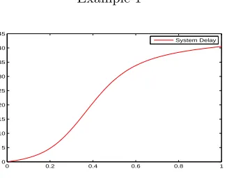
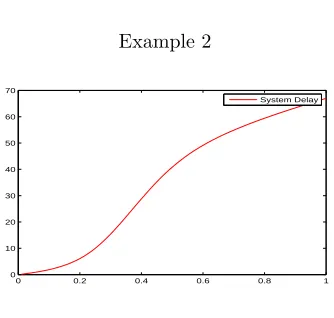
It is natural to ask to what extent the usual finite state truncation really destroys structural properties. The usual finite state truncation limits the state space to a finite set parameterized by N, and the transition probabilities leading towards states out of this set and mapped back to some state inside the set. Sennott ([8], Section C4 and C5) shows that the average expected cost under the truncated model converges to the average expected cost of the original model as

N tends to infinity. However, the following examples show that the structural properties of the original model are lost in the finite-state truncations.

In the following, we calculate and plot the system delay cost,gs, as a function of s∈ (0,1].

We truncate the state space to the set{0, . . . ,20} × {0, . . . ,50}. In the two examples we see that

gs is increasing in s, however,gs lacks convexity. As seen, convexity is not preserved under this

truncation. In some cases, ad-hoc choices of the transition rates on the boundaries do preserve structural properties of the relative value function (see, e.g., Down et al. [2]). Their approach does not apply to our model.

Example 1

0 0.2 0.4 0.6 0.8 1

0 5 10 15 20 25 30 35 40 45

System Delay

Example 2

0 0.2 0.4 0.6 0.8 1

0 10 20 30 40 50 60 70

System Delay

Figure 2: λ= 50, µ= 10, β = 10, γ= 10, ψ= 0.9, and R= 1.

References

[1] H. Blok and F.M. Spieksma. Continuity and ergodicity properties of a parametrised collection of countable state Markov processes. In preparation, 2013.

[2] D.G. Down, G.M. Koole, and M.E. Lewis. Dynamic control of a single server system with abandonments. Queueing Systems, 69:63–90, 2011.

[3] X. Guo and O. Hern´andez-Lerma. Continuous-Time Markov Decision Processes. Springer-Verlag Berlin Heidelberg, 2009.

[4] A. Hordijk and F.M. Spieksma. On ergodicity and recurrence properties of a Markov chain with an application to an open Jackson network.Advances in Applied Probability, 24:343–376, 1992.

[5] G.M. Koole. Monotonicity in Markov reward and decision chains: Theory and applications.

Foundations and Trends in Stochastic Systems, 1:1–76, 2006.

[6] S. Lippman. Applying a New Device in the Optimization of Exponential Queuing Systems.

Operations Research, 23:687–709, 1975.

[7] R.B. Lund, S.P. Meyn, and L. Tweedie. Computable exponential convergence rates for stochastically ordered Markov processes. Annals of Applied Probability, 6(1):218–237, 1996.

[8] L.I. Sennott. Stochastic Dynamic Programming and the Control of Queueing Systems. John Wiley & Sons, 1999.

[9] R.F. Serfozo. An equivalence between continuous and discrete time Markov Decision Pro-cesses. Operations Research, 27(3):616–620, 1979.