Journal of Hydraulic Structures J. Hydraul. Struct., 2020; 6(1): 33-54
DOI: 10.22055/jhs.2020.31685.1125
Air flow effect on the behavior of lock-exchange gravity
current
Ali Koohandaz
1 Ehsan Khavasi2Hamid Yousefi3
Hossein Sadeghi Sarsari1
Abstract
The main goal of this study is investigating the effect of air flow above the free surface on the behavior of gravity current. Lock-release gravity current has been simulated in a channel, by using VOF method, for modeling free surface at the interface of gas and liquid phases. Eulerian approach is used to consider the presence of particles in the flow. The results of simulation with free surface assumption are in a well agreement with the previous experimental results. It is observed that the flows containing particles with larger diameter experience higher deposition rate, due to their higher terminal velocities which are 0.000129m/s, 0.000359m/s and 0.000808m/s for the particles with 12μm, 20μm and 30μm diameters respectively. Increasing the size of particles diameter leads to decrease in the driving force, the front position of flow containing particles with 30μm diameter is 11% less than that of flow containing particles with 12μm diameter, thereby the flow velocity decays quickly. The results show that the presence of particles leads to a reduction in the value of entrainment rate. It is concluded that the velocity of air-phase affects the shape of flow and instabilities. By considering three different values of 0.1m/s, 0.12m/s and 0.18m/s for the air-phase velocity, it is observed that the amount of run-out length, in the case where the air velocity is 0.18m/s, is nearly 3% more than that in other cases at the end of channel, moreover it leads to an increase in the value of entrainment rate.
Keywords: Gravity current, lock exchange, multiphase flows, free surface, large eddy simulation.
Received: 12 November 2019; Accepted: 23 January 2020
1 Faculty of Mechanical engineering ,University of Zanjan, Zanjan,Iran
2 Faculty of Mechanical engineering ,University of Zanjan, Zanjan,Iran. [email protected]
(Corresponding author)
1. Introduction
Gravity currents are formed by difference in the density of two fluids, which can be due to the difference in temperature, salinity or particle suspension [1, 2]. Indeed, the density differences cause the horizontal hydrostatic pressure gradients [3]. Salinity and temperature are the causes of density gradients in homogeneities and suspended material is the cause of density gradient in turbidity currents [4]. Density currents can widely be found in nature (oceanic overflows, sea breeze fronts, avalanches, submarine landslides) [5]. In reservoirs, sediment deposition from turbidity currents leads to storage capacity loss [6]. They have an important role in the sediment transport when they propagate in the lakes and oceans [7]. The density contrast is usually small, consequently the Boussinesq approximation is appropriate to study the problem, hence this assumption is applied in this study. Most efforts to obtain an intuitive understanding of the dynamics of gravity currents, have done by means of laboratory experiments [8 - 13]. In recent years, with the improvement of computational methods, researchers have tended to conduct fully three-dimensional, depth-resolved simulations of gravity currents [14 - 19].
In the other hand, in the propagation of gravity current, boundary conditions are effective parameters in the transition from laminar to turbulent flow and also in the mixing processes, for example, if the wall boundary condition is assumed to be solid, lobe-cleft instability has an important role for the transition, in the frontal region. It should be mentioned that the lobe-cleft instability is created because of the unstable stratification due to the lifting of nose from the wall and the movement of ambient fluid under the gravity current, if the boundary condition is shear-free, lobe-cleft instability will not occur [20], for example, when an oil spreads over the surface of the ocean [21].
Many researchers have accomplished experimental studies, or numerical investigations with various boundaries. The type of boundaries are classified into no-slip and slip conditions, in other words, wall and free surface boundary conditions [20].
Many studies have examined gravity currents in a channel with different boundary conditions, for example when the top and bottom boundaries are walls [14, 22, 23, 24], or when both the upper and lower boundaries have slip or no-slip condition [25, 26]. Longo et al. [27] have performed experiments on inertial gravity currents advancing ambient fluid without top lid. Some studies have been done in order to determine the effect of wave on the characteristics of gravity current [28, 29], for example Viviano et al. [29] have investigated the wave influence on shape of the interface between gravity current and ambient fluid, mixing, turbulence, velocity and vorticity fields. The roughness of the bed, has affected the problem, when the wall boundary conditions is applying [30 - 34]. In this paper, smooth walls are considered. It should be mentioned that when the gravity current is in shallow ambient fluid, the upper boundary condition is more effective on the dynamics of flow than when the gravity current is in a deep ambient fluid, so considering top boundaries as free surface instead of wall, in shallow ambient fluid, will change the behavior of gravity current.
Liu and Jiang [20], investigated the impact of various depth ratio, on the Boussinesq gravity current in the wall-bounded and open channels by both laboratory experiments and numerical simulation. In addition, they analyzed the effect of propagation speed of density current on the lobe-cleft instability, Kelvin-Helmholtz billows, and the height of the gravity current. They also explored the impact of boundary conditions on the energy dissipation.
Ottolenghi et al. [36], have investigated the behavior of lock-release gravity current, experimentally and numerically. Their focus was mostly on the speed of current propagation, during the early stages after the flow formation. There was a good match between the results of experiments with that of simulations which has been done by LES model with considering shear-free for top boundary.
An important point to be noted with regard to the above studies is the fact that not much researches have focused on the effect of free-surface boundary condition on gravity current in the simulations. Noticeably, Liu [20] compared density current in two different conditions: wall-bounded and open channels by means of direct numerical simulation, in addition, the lobe-cleft instability, Kelvin-Helmholtz billows, and the effect of density current height were investigated. They showed that the boundary conditions change the turbulent flow field and the propagation of the front. With the decrease of initial release depth ratio (D/H), (where D is the depth of dense fluid and H is the channel depth), the effect of the top boundary becomes less important.
Many different researches have been done to simulate the gravity current in the channel by numerical methods. In reality, the air above the surface of the surrounding water containing gravity current mostly flows over the free surface. To the best of authors’ knowledge there is no research considers the air flow above the surrounding water. So, this issue selected as the main novelty of this paper. The effect of the air flow on the behavior of gravity and turbidity current is studied numerically with the aim of LES turbulence model in OpenFOAM. To model the free surface between the air and water VOF (Volume of Fluid) method is applied. To produce gravity (or turbidity current) the concentration equation (with Stokes settling velocity) is added to the interFoam solver. To check the free surface validity a part of the paper discusses about the effect of this type of boundary condition comparing with result of previous experimental studies. The effect of particle size on the general behavior of the current and depositional trend is also investigated. The effect of mentioned parameters (such as the air flow and particles) on the entrainment is studied, too.
Section. 2 formulates the governing equations and also the modeling approach has been presented. Section. 3 focuses on discussion and comparison of the numerical results and, finally, section. 4 summarizes findings and also main conclusions of investigation has expressed.
.
2. Methodology
2.1. Physical model and governing equations
As mentioned previously Boussinesq approximation will be taken into consideration to solve the Navier-Stokes equations (i.e. if the difference of the gravity current with the ambient fluid is low enough, by assuming a constant density equal to the reference density, except in the gravity-buoyancy term of the momentum equations [37]).
The Navier-Stokes equations which is adopted to model the motion of flow, plus a transport equation for the Eulerian description of the concentration field is presented:
0 k k u x =
(1)
(
)
2 ' 211
2
pl l l
w SGS
k lk
w
k k k k l
u
u
u
u
S
g c
t
x
x
x
x
x
+
=
+
−
−
(2)
2 2
S k
V
n n n n n
SGS k
k k k k k k
c
u
c
c
c
c
t
x
x
x
x
x
x
+
+
=
+
(3)
Here 𝜌𝑊 and 𝜈𝑤 are the density and kinematic viscosity of ambient fluid, respectively.𝑔′ is
reduced gravity acceleration 𝑔′= 𝛽𝑔 where 𝛽 =(𝜌−𝜌𝜌 𝑤)
𝑤 . Concentration is defined as 𝐶 =
(𝜌−𝜌𝑤)
(𝜌𝑚𝑎𝑥−𝜌𝑤) where 𝜌 is density of the current. In the concentration equation, 𝑉𝑠 is the terminal
settling velocity which takes the following form:
2 18
P w
s p
V gD
−
=
(4)
where μ is fluid viscosity and 𝐷𝑝 is particle diameter. 𝜌𝑤 is the density of ambient fluid and
𝜌𝑝 is the density of particles. The Schmidt number 𝑆𝑐 =𝜈𝛼 is the ratio of the kinematic viscosity
𝜈 𝛼 𝑆𝑐 ≥ 1
properties [37 - 39], hence its value is considered to be 𝑆𝑐 = 1 .In the LES method, Subgrid-scale eddy viscosity, 𝜈𝑆𝐺𝑆 ,is modeled, therefore by having turbulent Schmidt number 𝑆𝑐𝑆𝐺𝑆
equal to one [25, 40], 𝛼𝑆𝐺𝑆 will be computed through the equation:
SGS SGS
SGS
Sc
=
(5)
It should be noted that in this paper, spherical particles with three different diameters (12, 20 and 30μm) have been used. The density of the particles is taken as 2650kg/m3in all runs which indicates that the type of particles is kaolin. Deposition profile is a criterion to show the deposition behavior of current and it can be assessed in each section of the channel and compared with its value at the entrance:
0
( , )
s w s
Q C x t V dt
=
(6)
In abovementioned relation the values of terminal settling velocity and concentration are that of near the channel bed.
VOF model is a technique for simulation of free surface using a fixed mesh. This method is designed for simulation of two or more immiscible fluids. The formulation of the VOF model is based on the principle that different phases are not combined together. In this method identifying the location of the interface between two fluids is the main object [35].
Actually, the interface between two fluids is followed implicitly in this method. Fundamentally, in VOF model, the boundary is determined from the quantity of α called volume fraction, which is stored in the computational cells in domain, and it determines which fluid exist in the cells. In this study, in a cell filled with water, the value of α is equal to 1, and in a cell void of water and filled with air, α is equal to 0. In the cells of interface, which is between two phases, α is between 0 and 1. The advantage of this method is solving the governing equations on the fluid with considering the boundary in cells that makes it easier to apply. Identifying the boundary between phases is done by solving a transport equation for volume fraction. This equation is as follows [41]:
.( V) 0
t
+ =
(7)
For each computational cell in the domain, the average fluid properties for density and viscosity are calculated by [41]:
(8)
1 (1 ) 2
= + −
(9)
1 (1 ) 2
= + −
.( V ) .Vr (1 ) 0
t
+ + − =
(10)
Where 𝑉𝑟 , is the relative velocity between two phases and 𝑉̄ is calculated by weighted average of two fluids velocities, as follows:
1 2
r
V =V −V
(11)
1
(1
)
2V
=
V
+ −
V
(12)
With considering the effect of free-surface, momentum equations have form [43]:
( )
.( ) ( ). .( ) ST
V
V V p g V V F
t
+ = − + + + +
(13)
Where 𝐹𝑆𝑇 is the surface tension force which is obtained by:
ST
F =
k
(14)
in abovementioned relation,
is surface tension coefficient andk
is the curvature, calculated by: . k
=
(15)
In this paper the amount of entrainment is also calculated. The dimensionless number 𝐸𝑖_𝑏𝑢𝑙𝑘
which is a criterion to measure entrainment, is expressed as:
_ _
2
ei i bulk i bulkW
E
U
=
(16)
Where the 𝑈𝑖_𝑏𝑢𝑙𝑘 is the bulk velocity which indicates the velocity of gravity current head, and
𝑊𝑒𝑖 is entrainment velocity:
ei ei i
Q
W
S
=
(17)
In aforementioned relation, 𝑄𝑒𝑖 is the bulk entrainment discharge:
i ei i
V
Q
t
=
(18)
In fact, Qei is the rate of separated fluid volume from the ambient fluid volume in each time
step. Each volume in each time step, is calculated by the MeshLab software, which is used for geometrical computation.
In relation (17), 𝑆𝑖 is the interface and is obtained by multiplying the width of channel 𝑑 and location of current head 𝑥𝑓:
.
i f
In the other hand in this study Reynolds number defined as:
0
Re
H
g H
=
(20)
where 𝑔0′ is reduced gravity, H is the height of ambient fluid, and 𝜈 is the viscosity of water.
The interaction between gravity current and the particles is considered to be a one-way coupling, based on the assumption that the effect of particles on the turbulent flow is negligible due to low particle loading. In the other words, the value of particle volume fraction (calculated by Eq. 21) is less than 10−6, accordingly the effect of turbulent flow on the particles is predominant, and the effect of particles on the behavior of turbulent flow is considered negligible [38].
P p
MV V
=(21)
Here 𝑉 denotes the volume of fluid and particles, 𝑉𝑃 is the volume of particle and 𝑀 is
number of particles.
2.2 Numerical methods
The computational domain size is 600 × 60 × 40, respectively, in the streamwise, bottom wall-normal, and spanwise directions. In order to resolve viscous sub-layer, the height of first cell near the wall, should be sufficient, which has traditionally been studied by 𝑦+as the dimensionless distance from the wall [37]:
u y y
+ = (22)
where: wu
=
(23)
𝑦+ nearly equal to 1, is sufficient to capture the viscous sub-layer [45], so this value is
considered for 𝑦+ in the present work.
No-slip condition is considered at the walls. The concentration of gravity current has a uniform value of 0.8 in the initial condition for the all runs. For the velocity of the air-phase at the free-surface, three different values of 0.1m/s, 0.12m/s and 0.18m/s are applied.
Reynolds number is more than 1000 in the all cases, which is the critical Reynolds number based on initial height of gravity current, it shows that the effect of viscosity is negligible and it ensures that the flow is turbulent [36].
More than 16 cells in the geometry is a minimum number of cells, for having an accurate LES and representing the largest structures of flow. Therefore the maximum mesh size should be scale with 16𝐻 where 𝐻 is the height of the lock part, while the minimum mesh size of an LES should be higher than the Kolmogorov length scale, which is defined based on the energy
cascade theory of homogeneous turbulence, as (𝐻2) 𝑅𝑒−
3
4 [37]. Hence, the mesh size h should be
in the size range of (𝐻
2) 𝑅𝑒
−3
4 ≤ℎ< 𝐻
In order to discretize the divergence terms in equations, Gauss linear method, Gauss QUICK method, Gauss limited linear method, Gauss LUST method and Van Leer method are utilized, in addition to discretize the Laplacian terms, modified Gauss linear, are used. QUICK method is a fourth order method for the gradient term a fourth order method presented by Peer et al. [46] has been employed meanwhile time discretization scheme is a backward second order method [17].
2.3 validation
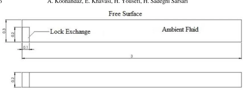
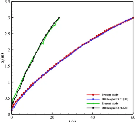
Experimental results obtained by Ottolenghi et al. [36] are used in order to validate the numerical simulations of this study. Figure. 2 shows the comparison between the profiles of gravity current head location at various times, obtained by Ottolenghi et al. [36] and the profiles of present simulations. The length and width of the lock part can change, due to the release conditions, beside these variables, reduced gravity acceleration is another factor which is changed by Ottolenghi et al. [36]. In the following, the effect of combination of these changes has been investigated and the profiles of head locations have been compared. In the investigation of Ottolenghi et al. [36], depth ratio (the ratio of lock height to lock length) and reduced gravity in exp1, were 2 and 0.01529m/s2, also 1 and 0.06014m/s2 in exp2, respectively. These two cases are simulated in the present study, too. The comparison of the results is shown in figure 2. The difference of the present study results with the experimental results of [36] is in order of 2%. So, the numerical results have acceptable accuracy. It should be noted that in the numerical simulations the total height of the channel is 0.3m in which the lock height is 0.2m and the remaining is the air phase.
Figure 2. Comparison between profiles of gravity current head location at various times, obtained from numerical simulation of this study, and experimental results obtained by Ottolenghi
et al. [36].
t (s)
xf
(m
)
0 20 40 60
0 0.5 1 1.5 2 2.5 3 3.5
3. Results and discussions
3.1. Effect of particles
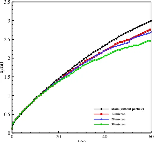
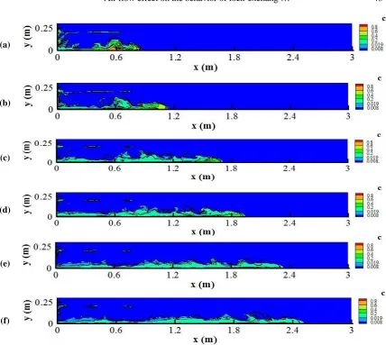
In this section, the effect of particles on the flow is studied, and like the previous section, VOF method is used to simulate free surface. In order to assess the effect of particles on the flow structure, Stokes terminal velocity is added to the concentration equation, and the flow behavior in the presence of particles with diameters of 12μm, 20μm and 30μm has been investigated. Figure 3 compares the front location of no particle gravity current with particulate gravity current (turbidity current) with various particle diameters.
Figure 3. Comparison of the front positions of gravity current containing particles with (a) red line: 12μm, (b) blue line: 20μm, (c) green line: 30μm diameter, and (d) black line: the case without
particle, in the channel with considering free-surface boundary condition
By observing figure 3, it is clearly seen that the temporal evolution of flow has been similar in all cases by t=14s, but after that the trend has changed. It is also possible to observe that the particles with 30μm diameter sediment quickly, because of their higher weight, and dense flow have lost its driving force, due to lowering the density contrast. Thus, the flows containing particles with 12μm and 20μm diameters, have travelled more quickly along the channel, in comparison with turbidity current containing particles with 30μm diameter. As shown in figure 4, the front position of flow, where the particles have 30μm diameter, is reduced by 11%, compared to the case with 12μm particle diameter. The deposition profiles of the particles in the flow obtained by the relation (6) for these three cases are illustrated in figure 4. In the cases where the suspended particles are 12μm, 20μm and 30μm, the values of Stokes terminal velocity are 0.000129m/s, 0.000359m/s and 0.000808m/s respectively. 𝐶𝑤(𝑥, 𝑡) is the value of flow concentration near the channel bed and can be obtained in each section of channel. In order to
t (s)
xf
(m
)
0 20 40 60
0 0.5 1 1.5 2 2.5 3 3.5
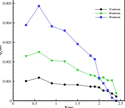
observe the deposition profile, 12 cross-sections along the channel are chosen at all times. In figure 4, the effect of particle diameter on the depositional behavior of the current, along the channel is investigated.
Figure 4. Comparison of the deposition profiles of particles with (a) black line: 12μm (b) green line: 20μm and (c) blue line: 30μm, in the channel with considering free-surface boundary condition.
Larger particles sediment faster because of their higher weight, therefore in a certain length of channel, the value of sediment deposition in a flow containing particles with larger diameters, is more than the case with smaller particle diameter. Since density contrast in the flows containing larger particles, is reduced quickly, due to the fast deposition of its particles, driving force of gravity current is decreased, thereby flow advancement of gravity current with larger particle diameter is slower than that of gravity current with smaller particle diameter. As a result, the value of deposition of particles with 30μm diameter, reaches the value of 0, faster than other cases, (see figure 4). Contours of concentration for flows containing particles with 12μm and 30μm diameters, are depicted in figures 5 and 6, respectively.
X(m)
Q
s
(m
)
0 0.5 1 1.5 2 2.5
0 0.001 0.002 0.003 0.004 0.005
(a)
(b)
(c)
(d)
(e)
(f)
(a)
(b)
(c)
(d)
(e)
(f)
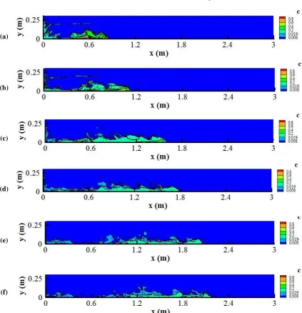
Figure 6. The evolution of gravity current, containing particles with 30μm diameter, visualized by concentration contours. Results for (a) t=12s, (b) t=18s, (c) t=30s, (d) t=36s, (e) t=48s and (f) t=54s.
(a)
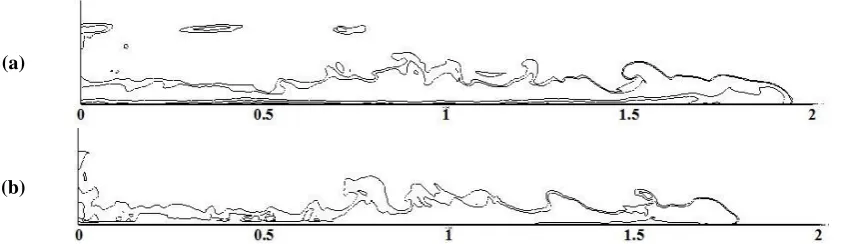
(b)
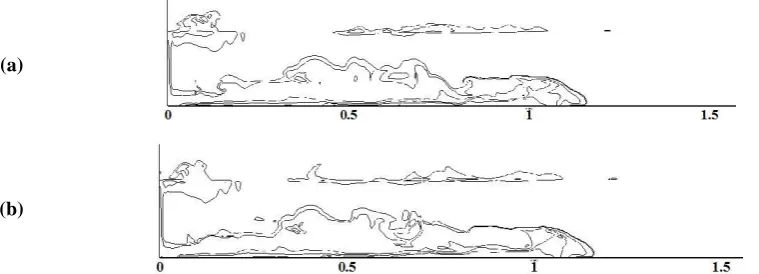
Figure 7. Concentration contours of gravity current containing particles with (a) 12μm and (b) 30μm diameters, with considering free-surface boundary condition, from side view of the channel, after 18 seconds.
(a)
(b)
Figure 8. Concentration contours of gravity current containing particles with (a) 12μm and (b) 30μm diameters, with considering free-surface boundary condition, from top view of the channel,
after 18 seconds.
(a)
(b)
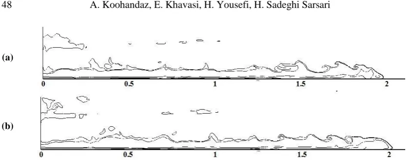
Figure 9. Concentration contours of gravity current containing particles with (a) 12μm and (b) 30μm diameters, with considering free-surface boundary condition, from side view of the channel,
(a)
(b)
Figure 10. Concentration contours of gravity current containing particles with (a) 12μm and (b) 30μm diameters, with considering free-surface boundary condition, from top view of the channel,
after 36 seconds.
In figures 7 to 10, it is observed that there is no significant difference between the two flows with different particle diameters up to 18s, but after that the differences are remarkable. First of all, it can easily be seen that the front location of turbidity current containing larger particles fall behind the flow with smaller particle. The second point is that the thickness and size of the head reduces as the particle diameter increases.
3.2 Effect of air-phase velocity at the free surface
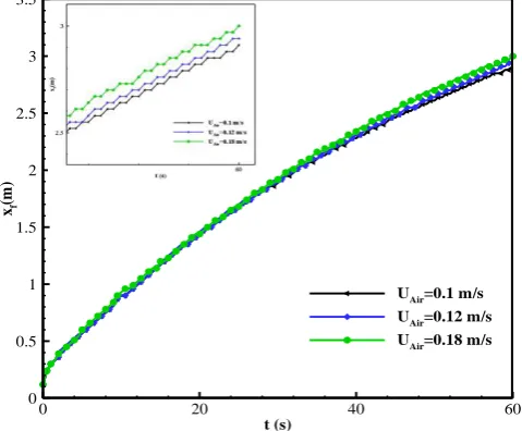
As said before the main goal of this study is considering the effect of air flow on the free surface on the behavior of gravity current. So, in this section the impact of air-phase velocity at the free surface when the airflow over the fluid-phase enters the left side of the channel is studied by investigating front position, concentration contours and comparing the structure of gravity current in different cases. For this purpose, three different values for the air-phase velocity are taken into account. Figure 11 shows variation of the front location of gravity current with time in three different values of 0.1m/s, 0.12m/s and 0.18m/s for the air-phase velocity.
Figure 11. Variation of the front position of gravity current with time. Results for (a) 0.1m/s air velocity, (b) 0.12m/s air velocity and (c) 0.18m/s air velocity.
t (s)
xf
(m
)
0 20 40 60
0 0.5 1 1.5 2 2.5 3 3.5
UAir=0.1 m/s
UAir=0.12 m/s
According to figure 11 the temporal evolution of flow is same for all cases until t=30s, and then flow velocity increases with increasing the air velocity. As a result, the value of run-out length, in the case where the air velocity is 0.18m/s, is approximately 3% more than that in other cases, at the end of channel. In order to obtain a better understanding of the effect of the air-phase velocity general shape of the flow structure for two cases where the values of air-air-phase velocity are 0.18m/s and 0.1m/s are compared at the 18s, 36s and 48s and shown in figures 12-17 from front and top views.
(a)
(b)
Figure 12 . Concentration contours of gravity current considering the values of (a) 0.1m/s and (b) 0.18m/s for the air-phase velocity, from side view of the channel, at the 18s.
(a)
(b)
(a)
(b)
Figure 14. Concentration contours of gravity current considering the values of (a) 0.1m/s and (b) 0.18m/s for the air-phase velocity, from side view of the channel, at 36s.
(a)
(b)
Figure 15. Concentration contours of gravity current considering the values of (a) 0.1m/s and (b) 0.18m/s for the air-phase velocity, from top view of the channel, at 36s.
(a)
(b)
(a)
(b)
Figure 17. Concentration contours of gravity current considering the values of (a) 0.1m/s and (b) 0.18m/s for the air-phase velocity, from top view of the channel, at 48s.
By observing figures 12 to 17 it can be seen that the variations in the structure of flow consist of the nose and the body as well as the instabilities due to the change in the value of air-phase velocity are not significant. Just, the location of the head changes with the air flow at the top boundary. This could be due to the extra momentum induced by air flow into the ambient water and then gravity current.
3.3 Entrainment rate
One of the most considerable problems, in context of gravity current is the entrainment of ambient fluid into the current. At the interface of two fluids due to existence of interfacial shear stress, lighter ambient fluid is pushed into the denser fluid, and it leads to the mixing, increasing flow height and reducing the driving force. This section aimed to shed light on the entrainment of gravity current. The assessment of the amount of entrainment is an important factor in the numerical simulation of gravity current. The amount of entrainment is generally expressed by the dimensionless parameter, called entrainment factor [36] which is calculated by relation (16). As shown in figure 18, In all runs, the height of the lock part is considered to be equivalent to two-third of the h, and one-third of h is occupied by the air-phase, where h is the height of channel.
Figure 18. Schematic of sections occupied by the air and water phases.
Figure 19. Entrainment factor of the gravity current in the channel with the heights of (a) 0.5m and (b) 0.3m, as well as (c) considering the value of 0.12m/s for the air-phase velocity.
The results, indicates that the rate of entrainment decreases with evolution of flow. It also shows that the air-phase velocity causes a significant enhancement in the value of entrainment, due to the increasing of the driving force, especially in the early stages of the flow advancement.
Figure 20. Entrainment factor of gravity current, containing particles with (a) 30μm and (b) 12μm diameter, [with considering free surface boundary condition].
In figure 20, it can be observed that the flow containing particles with larger diameter has less
xf/H
Ei_
b
u
lk
0.2 0.3 0.4 0.5 0.6 0.7
0 0.015 0.03 0.045 0.06
UAir=0.12 m/s
Channel Height=0.3 m
Channel Height=0.5 m
xf/H Ei_
b
u
lk
0.2 0.3 0.4 0.5 0.6 0.7
0 0.02 0.04 0.06 0.08
instabilities are obviously decreased and flow experiences higher deposition rate and thereby gravity current decays quickly.
4. Conclusion
The main goal of this paper was studying numerically the effect of wind or air flow above the ambient water of the lock-release gravity current. As this condition needs to consider both phases of water and air VOF method has been employed to model the interface of the water and air. In order to assess the effect of particles on the structure of flow, the numerical simulation of the flow, with and without considering particles has been carried out. Eulerian approach has been used to consider the existence of the particles. In the flow containing particles, driving force is reduced due to increasing the size of particles diameter and subsequently decreasing density contrast. As a result, particles with larger diameter, deposit faster and flow decays quickly. In the next step, the effect of various air-phase velocities on gravity current have been studied. With increasing the value of air-phase velocity, the value of run-out length increases, in addition it was observed that the velocity of air-phase, affects the formation of instabilities. Finally, entrainment rate has been studied, the results show reduction of entrainment rate with evolution of flow on the channel bed. It was found that the air-phase velocity causes an enhancement in the value of entrainment, due to increasing the driving force. Another result is that the flow containing particles with larger diameter has less entrainment rate.
5. References
1. Khavasi, E., & Firoozabadi, B. (2019). Linear spatial stability analysis of particle-laden stratified shear layers. Journal of the Brazilian Society of Mechanical Sciences and Engineering, 41(6), 246.
2. Khavasi, E., & Firoozabadi, B. (2018). Experimental study on the interfacial instability of particle-laden stratified shear flows. Journal of the Brazilian Society of Mechanical Sciences and Engineering, 40(4), 193.
3. Nasr-Azadani, M. M., Meiburg, E., & Kneller, B. (2018). Mixing dynamics of turbidity currents interacting with complex seafloor topography. Environmental Fluid Mechanics, 18(1), 201-223.
4. Kyrousi, F., Leonardi, A., Roman, F., Armenio, V., Zanello, F., Zordan, J., Juez, C., & Falcomer, L. (2018). Large Eddy Simulations of sediment entrainment induced by a lock-exchange gravity current. Advances in Water Resources, 114, 102-118.
5. Ottolenghi, L., Adduce, C., Roman, F., & Armenio, V. (2019). Analysis of the flow in gravity currents propagating up a slope. International Journal of Sediment Research, 34(3), 240-250.
6. Zhao, L., Yu, C., & He, Z. (2019). Numerical modeling of lock-exchange gravity/turbidity currents by a high-order upwinding combined compact difference scheme. International Journal of Sediment Research, 34(3), 240-250.
8. Bonnecaze, R. T., Huppert, H. E., & Lister, J. R. (1993). Particle-driven gravity currents. Journal of Fluid Mechanics, 250, 339-369.
9. De Rooij, F., & Dalziel, S. (2001). Time‐and space‐resolved measurements of deposition under turbidity currents. Particulate gravity currents, 207-215.
10. Gladstone, C., Phillips, J., & Sparks, R. (1998). Experiments on bidisperse, constant-volume gravity currents: propagation and sediment deposition. Sedimentology, 45(5), 833-843.
11. Kane, I. A., McCaffrey, W. D., Peakall, J., & Kneller, B. C. (2010). Submarine channel levee shape and sediment waves from physical experiments. Sedimentary Geology, 223(1-2), 75-85.
12. Luthi, S. (1981). Experiments on non-channelized turbidity currents and their deposits. Marine Geology, 40(3-4), M59-M68.
13. Peakall, J., Amos, K. J., Keevil, G. M., Bradbury, P. W., & Gupta, S. (2007). Flow processes and sedimentation in submarine channel bends. Marine and Petroleum Geology, 24(6-9), 470-486.
14. Cantero, M. I., Balachandar, S., Cantelli, A., Pirmez, C., & Parker, G. (2009). Turbidity current with a roof: Direct numerical simulation of self‐stratified turbulent channel flow driven by suspended sediment. Journal of Geophysical Research: Oceans, 114(C3).
15. Huang, H., Imran, J., & Pirmez, C. (2008). Numerical study of turbidity currents with sudden-release and sustained-inflow mechanisms. Journal of Hydraulic Engineering, 134(9), 1199-1209.
16. Kassem, A., & Imran, J. (2004). Three-dimensional modeling of density current. II. Flow in sinuous confined and uncontined channels. Journal of Hydraulic Research, 42(6), 591-602. 17. Nasr-Azadani, M. M., & Meiburg, E. (2011). TURBINS: an immersed boundary, Navier– Stokes code for the simulation of gravity and turbidity currents interacting with complex topographies. Computers & Fluids, 45(1), 14-28.
18. Necker, F., Härtel, C., Kleiser, L., & Meiburg, E. (2002). High-resolution simulations of particle-driven gravity currents. International Journal of Multiphase Flow, 28(2), 279-300. 19. Necker, F., Härtel, C., Kleiser, L., & Meiburg, E. (2005). Mixing and dissipation in
particle-driven gravity currents. Journal of Fluid Mechanics, 545, 339-372.
20. Liu, X., & Jiang, Y. (2014). Direct numerical simulations of boundary condition effects on the propagation of density current in wall-bounded and open channels. Environmental Fluid Mechanics, 14(2), 387-407.
21. Scotti, A. (2008). A numerical study of the frontal region of gravity currents propagating on a free-slip boundary. Theoretical and Computational Fluid Dynamics, 22(5), 383 22. Benjamin, T. B. (1968). Gravity currents and related phenomena. Journal of Fluid
Mechanics, 31(2), 209-248.
24. Séon, T., Znaien, J., Salin, D., Hulin, J., Hinch, E., & Perrin, B. (2007). Transient buoyancy-driven front dynamics in nearly horizontal tubes. Physics of Fluids, 19(12), 123603.
25. Härtel, C., Meiburg, E., & Necker, F. (2000). Analysis and direct numerical simulation of the flow at a gravity-current head. Part 1. Flow topology and front speed for slip and no-slip boundaries. Journal of Fluid Mechanics, 418, 189-212.
26. Bonometti, T., Balachandar, S., & Magnaudet, J. (2008). Wall effects in non-Boussinesq density currents. Journal of Fluid Mechanics, 616, 445-475.
27. Longo, S., Ungarish, M., Di Federico, V., Chiapponi, L., & Petrolo, D. (2018). Gravity currents produced by lock-release: theory and experiments concerning the effect of a free top in non-Boussinesq systems. Advances in Water Resources,121, 456-471.
28. Musumeci, R. E., Viviano, A., Foti, E. (2017). Influence of Regular Surface Waves on the Propagation of Gravity Currents: Experimental and Numerical Modeling. Journal of Hydraulic Engineering, 143(8), 04017022.
29. Viviano, A., Musumeci, R. E., & Foti, E. (2018). Interaction between waves and gravity currents: description of turbulence in a simple numerical model. Environmental Fluid Mechanics, 18(1), 117-148.
30. Dallimore, C. J., Imberger, J., & Ishikawa, T. (2001). Entrainment and turbulence in saline underflow in Lake Ogawara. Journal of Hydraulic Engineering, 127(11), 937-948.
31. Fernandez, R. L., & Imberger, J. (2006). Bed roughness induced entrainment in a high Richardson number underflow. Journal of Hydraulic Research, 44(6), 725-738.
32. Hebbert, B., Patterson, J., Loh, I., & Imberger, J. (1979). Collie river underflow into the Wellington reservoir. Journal of the Hydraulics Division, 105(5), 533-545.
33. La Rocca, M., Adduce, C., Sciortino, G., & Pinzon, A. B. (2008). Experimental and numerical simulation of three-dimensional gravity currents on smooth and rough bottom. Physics of Fluids, 20(10), 106603.
34. Lauber, G., & Hager, W. H. (1998). Experiments to dambreak wave: Horizontal channel. Journal of Hydraulic Research, 36(3), 291-307.
35. Adduce, C., Sciortino, G., & Proietti, S. (2011). Gravity currents produced by lock exchanges: experiments and simulations with a two-layer shallow-water model with entrainment. Journal of Hydraulic Engineering, 138(2), 111-121.
36. Ottolenghi, L., Adduce, C., Inghilesi, R., Armenio, V., & Roman, F. (2016). Entrainment and mixing in unsteady gravity currents. Journal of Hydraulic Research, 54(5), 541-557. 37. Pelmard, J., Norris, S., & Friedrich, H. (2018). LES grid resolution requirements for the
modelling of gravity currents. Computers & Fluids, 174, 256-270.
38. Nasr-Azadani, M. M., & Meiburg, E. (2013). Influence of seafloor topography on the depositional behavior of bi-disperse turbidity currents: a three-dimensional, depth-resolved numerical investigation. Environmental Fluid Mechanics, 14(2), 319-342. i:10.1007/s10652-013-9292-5.
40. Härtel, C., Carlsson, F., & Thunblom, M. (2000). Analysis and direct numerical simulation of the flow at a gravity-current head. Part 2. The lobe-and-cleft instability. Journal of Fluid Mechanics, 418, 213-229.
41. Lopes, P. (2013). Free-surface flow interface and air-entrainment modelling using OpenFOAM.
42. Weller, H., & Derivation, M. (2005). Solution of the Conditionally Averaged Two-Phase Flow Equations. OpenCFD, Ltd.
43. Ketabdari, M. J. (2016). Free Surface Flow Simulation Using VOF Method. Numerical Simulation: From Brain Imaging to Turbulent Flows, 365.
44. Elghobashi, S. (1991). Particle-laden turbulent flows: direct simulation and closure models Computational fluid Dynamics for the Petrochemical Process Industry (pp. 104): Springer.
45. Ottolenghi, L., Adduce, C., Inghilesi, R., Roman, F., & Armenio, V. (2016). Mixing in lock-release gravity currents propagating up a slope. Physics of Fluids, 28(5), 056604. 46. Peer, A., Gopaul, A., Dauhoo, M., & Bhuruth, M. (2008). A new fourth-order