Homotopy Analysis Method for Equations of the Type Δ2=b(x,y) and Δ2u=b(x,y,u)

(1)

http://dx.doi.org/10.4236/jamp.2015.34049

Homotopy Analysis Method for Equations

of the Type

∇

2 u

=

b x y

(

,

)

and

(

)

2 _{, ,}

∇

u

=

b x y u

Selcuk Yildirim

Department of Electrical and Electronics Engineering, Siirt University, Siirt, Turkey Email: [email protected]

Received January 2015

Abstract

In this paper, the homoto pyanalysis method (HAM) is presented to solve some of engineering problems. The homotopy analysis method is applied in obtaining exact solutions for equations of

the type 2

(

)

,

∇ =u b x y and ∇2u=b x y u

(

, ,

)

on an elliptical domain. Exact solutions are presented

for several examples involving to demon strate the applic ability and efficiency of HAM.

Keywords

Homotopy Analysis Method, Engineering Problems, Exact Solutions

1. Introduction

The homotopy analysis method is developed in 1992 by Liao [1]-[8]. It is an analytical approach to get the series solution of linear and nonline arpartial differential equations. The difference with the other perturbation methods is that this method is independent of small/large physical parameters. It also provides a simple way to ensure the convergence of series solution [9]. This method has been successfully applied to solve many linear and non linear partial differential equationsin various fields of science and engineering by many authors [1]-[16]. The homotopy analysis method is useful and efficient for obtaining both analytical and numerical approximations of linear or nonlinear differential equations. In this study, we will concentrate on exact solutions for equations type of

( )

2

, u b x y

∇ = and ∇ =2u b x y u

(

, ,

)

frequently used in applied and engineering mathematics.

2. The Engineering Equations on an Elliptical Domain

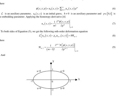
We refer to the problem given by Partridge and Brebbia [17]. Consider the following engineering equations

( )

2 2

2 2 ,

u u

b x y

x y

∂ ₊∂ ₌

(2)

(

)

2 2

2 2 , ,

u u

b x y u

x y

∂ ∂

+ =

∂ ∂ (2)

where b x y

( )

, , that is, considered to be a known function of position and b x y u

(

, ,

)

will be considered as a known function of the potential.

In all applications, the domain bounded by the ellipse given in Figure 1 will be used. The boundary condition is the Dirichlet condition with u=0 on the boundary.

The equation of the ellipse is

2 2

1 4

x y

+ = (3)

3. Homotopy Analysis Method

We apply the HAM to equations of the type ∇ =2u b x y

( )

, and ∇ =2u b x y u

(

, ,

)

with Dirichlet boundary condition. We consider the following differential equation

( )

, 0

N u x y_ _= (4)

where N is a linear operator, x and y are independent variables, u x y

( )

, is an unknown function. In HAM, the zeroth-orderde formation equation is constructed as

(

1−p

)



φ

(

x y p, ;

)

−u0

( )

x y, =p N 

φ

(

x y p, ;

)

 (5)

where

(

, ;

)

0

( )

, 1

( )

,

m m

m

x y p u x y u x y p

φ

∞

=

= +

∑

(6)

 is an auxiliary parameter, u₀

(

x y,

)

is an initial guess, ≠0 is an auxiliary parameter and p∈

[ ]

0,1 is the embedding parameter. Applying the homotopy-derivative [4]

( )

(

)

0

, ; 1

, !

m

m m

p

x y p u x y

m p

φ

=

∂ =

∂ (7)

To both sides of Equation (5), we get the following mth-order deformation equation

( )

, 1

( )

, 1

m m m m

u x y −

χ

u − x y = ℜ −

 

  

 (8)

where

(

)

(

)

1

1 1

0

, ; 1

1 !

m

m m

p

N x y p

m p

φ

−

− −

=

∂ _ _

ℜ =

− ∂ (9)

[image:2.595.94.541.336.709.2]

And

(3)

0, 1,

1, 1.

m

χ _{= } ≤

>

 (10)

Note that u_m

( )

x y, for m≥1 can be obtained by solving the linear Equation (8) with linear boundary con-ditions that come from original problem. If the power series Equation (6) of φ

(

x y p, ;

)

converges at p=1, then we gets the following series solution:

( )

, 0

( )

, m1 m

( )

,

u x y =u x y +

∑

∞₌u x y (11)

4. Applications

We apply Homotopy Analysis Method to equations of the type ∇ =2u b x y

( )

, and ∇ =2u b x y u

(

, ,

)

, as fol-lows:

Equation (1) suggests that we define an equation of linear operator as

(

)

2

(

2

)

2

(

2

) ( )

, ; , ;

, ; x y p x y p ,

N x y p b x y

x y

φ φ

φ =∂ +∂ +

 

  _∂ _∂ (12)

And Equation (2) suggests that we define an equation of linear operator as

(

)

2

(

2

)

2

(

2

)

(

)

, ; , ;

, ; x y p x y p , , , ;

N x y p b x y x y p

x y

φ φ

φ =∂ +∂ + φ

 

  _∂ _∂ (13)

Using the above definitions, the zeroth-orderde formation equation is constructed as

(

1−p

)



φ

(

x y p, ;

)

−u0

( )

x y, = p N 

φ

(

x y p, ;

)



Applying the homotopy-derivative to the zeroth-orderde formation equation, we obtain the following mth- orderde formation equations

( )

, 1

( )

, 1

m m m m

u x y −

χ

u − x y = ℜ −

 

  



Since m≥1, χ =m 1, now the solution of the mth-orderde formation equation becomes

( )

1

[

]

1 1

, ,

m m m

u x y =u − x y +− ℜ − (14)

where

( )

_{( ) ( )}

2 2

1 1

1 2 2

, ,

,

m m m

u x y u x y

b x y

x y

− −

−

∂ ∂

ℜ = + +

∂ ∂ (15)

( )

₍

_{( )}

₎

2 2

1 1

1 2 2 1

, ,

, , ,

m m

u x y u x y

b x y u x y

x y

− −

∂ ∂

ℜ = + +

∂ ∂ (16)

Example 1. Consider the equation of the type 2

u b

∇ =

2 2

2 2 2

u u

x y

∂ ₊∂ _{= −}

∂ ∂ (17)

With initial guess

( )

2

0

4 4

,

5 5

u x y = − y + (18)

using HAM, were cursively obtain

( )

2 0

( )

2 0

( )

1 0 0 2 0 0 2 0 0

, ,

, x x u x y d d x x u x y d d x x2d d

u x y x x x x x x

x y

∂ ∂

= + +

∂ ∂

∫ ∫

   (19)

( )

2

1

1 ,

5

(4)

( )

₀ ₀ 2 1

( )

2 1

( )

2 1 2 ₀ ₀ 2

, ,

, , x x u x y d d x x u x y d d

u x y u x y x x x x

x y

∂ ∂

= + +

∂ ∂

∫ ∫

  (21)

( )

(

2

)

2

1 ,

5

u x y =  + x (22)

( )

₀ ₀ 2 2

( )

2 2

( )

3 2 2 ₀ ₀ 2

, ,

, , x x u x y d d x x u x y d d

u x y u x y x x x x

x y

∂ ∂

= + +

∂ ∂

∫ ∫

  (23)

( )

(

2 3

)

2

3

1

, 2

5

u x y = +  + x (24)



( )

4 2 4 1 2

(

2

)

1 2

(

2 3

)

1 2

, 2

5 5 5 5 5

u x y = − y + + x +  + x + +  + x + (25)

When = −1, we obtain the exact solution as follows:

( )

1 2 4 2 4

,

5 5 5

u x y = − x − y + (26)

( )

4 2 2

, 1

5 4

x

u x y = − _ +y − _

  (27)

Example 2. Consider the equation of the type ∇ =2u b x y

( )

,

2 2

u u

x

x y

∂ ∂

+ = −

∂ ∂ (28)

with initial guess

( )

3

0

2 ,

14 7

x x

u x y = − + (29)

( )

₀ ₀ 2 0

( )

₀ ₀ 2 0

( )

₀ ₀

1 2 2

, ,

, y y u x y d d y y u x y d d y y d d

u x y y y y y x y y

x y

∂ ∂

= + +

∂ ∂

∫ ∫

   (30)

( )

2

1

2 ,

7 x

u x y = y (31)

( )

₀ ₀ 2 1

( )

2 1

( )

2 1 2 ₀ ₀ 2

, ,

, , y y u x y d d y y u x y d d

u x y u x y y y y y

x y

∂ ∂

= + +

∂ ∂

∫ ∫

  (32)

( )

(

2

)

2

2 ,

7 x

u x y =  + y (33)

( )

₀ ₀ 2 2

( )

2 2

( )

3 2 2 ₀ ₀ 2

, ,

, , y y u x y d d y y u x y d d

u x y u x y y y y y

x y

∂ ∂

= + +

∂ ∂

∫ ∫

  (34)

( )

(

2 3

)

2

3

2

, 2

7 x

u x y = +  + y (35)



( )

3 2 2 2

(

2

)

2 2

(

2 3

)

2 2

, 2

14 7 7 7 7

x x x x x

(5)

When = −1, we obtain the exact solution as follows:

( )

3 2 2 2

,

14 7 7

x x x

u x y = − + − y (37)

( )

2 2 2

, 1

7 4

x x

u x y = − _ +y − _

  (38)

Example 3. Consider the equation of the type _{∇ =}2_u _{b x y u}_{( , , )}

2 2

u u

u

x y

∂ ₊∂ _{= −}

∂ ∂ (39)

with initial guess

(

)

0 ,

u x y =x (40)

( )

₀ ₀ 2 0

( )

₀ ₀ 2 0

( )

₀

( )

1 2 2 ₀ 0

, ,

, x x u x y d d x x u x y d d x x , d d

u x y x x x x u x y x x

x y

∂ ∂

= + +

∂ ∂

∫ ∫

   (41)

( )

3

1 ,

3! x

u x y = (42)

( )

₀ ₀ 2 1

( )

₀ ₀ 2 1

( )

₀ ₀

( )

2 1 2 2 1

, ,

, , x x u x y d d x x u x y d d x x , d d

u x y u x y x x x x u x y x x

x y

∂ ∂

= + + +

∂ ∂

∫ ∫

   (43)

( )

(

2

)

3 2 5 2 ,

3! 5!

x x

u x y =  + + (44)

( )

₀ ₀ 2 2

( )

₀ ₀ 2 2

( )

₀ ₀

( )

3 2 2 2 2

, ,

, , x x u x y d d x x u x y d d x x , d d

u x y u x y x x x x u x y x x

x y

∂ ∂

= + + +

∂ ∂

∫ ∫

   (45)

( )

(

2 3

)

3

(

2 3

)

5 3 7

3 , 3 2

3! 5! 7!

x x x

u x y = +  +  +  + + (46)



( )

3

(

2

)

3 2 5

(

2 3

)

3

(

2 3

)

5 3 7

, 3 2

3! 3! 5! 3! 5! 7!

x x x x x x

u x y = +x  +  + + + +  +  +  + + + (47)

For = −1, we obtained the closed form series solution as

( )

, 3 5 7

3! 5! 7!

x x x

u x y = −x + − + (48)

(

,

)

sin

u x y = x (49)

which is the exact solution.

Example 4. Consider the equation of the type ∇ =2u b x y u

(

, ,

)

2 2

u u u

x

x y

∂ ₊∂ _{= −}∂ ∂

∂ ∂ (50)

with initial guess

( )

0 , 1

u x y = −x (51)

(6)

( )

2 0

( )

2 0

( )

0

( )

1 0 0 2 0 0 2 0 0

, , ,

, x x u x y d d x x u x y d d x x u x y d d

u x y x x x x x x

x x y ∂ ∂ ∂ = + + ∂ ∂ ∂

∫ ∫

   (52)

( )

2

1 ,

2! x

u x y = − (53)

( )

2 1

( )

2

( )

0 0 0 0

1 ₀

1

2 2 2 0

1

, , ,

, , x x u x y d d x x u x y d d x x u x y d d

u x y u x y x x x x x x

x x y ∂ ∂ ∂ = + + + ∂ ∂ ∂

∫ ∫

   (54)

( )

(

2

)

2 2 3

2 ,

2! 3!

x x

u x y = − +  − (55)

( )

2 2

( )

2

( )

0 0 0 0

2 ₀

2

3 2 2 0

2

, , ,

, , x x u x y d d x x u x y d d x x u x y d d

u x y u x y x x x x x x

x x y ∂ ∂ ∂ = + + + ∂ ∂ ∂

∫ ∫

   (56)

( )

(

2 3

)

2

(

2 3

)

3 3 4

3 , 2 2

2! 3! 4!

x x x

u x y = − +  + −  + − (57)



( )

2

(

2

)

2 2 3

(

2 3

)

2

(

2 3

)

3 3 4

, 1 2 2

2! 2! 3! 2! 3! 4!

x x x x x x

u x y = − −x  −  + − − +  + −  + − − (58)

( )

, 1 2 3 4

2! 3! 4!

x x x

u x y = − +x − + − (59)

( )

, e x

u x y = − (60) which is the exact solution.

Example 5. Consider the equation of the type ∇ =2u b x y u

(

, ,

)

2 2

u u u u

x y

∂ ∂ ∂ ∂

+ = − −

∂ ∂

∂ ∂ (61)

with initial guess

( )

0 , e 1

x

u x y = − + −y (62) using HAM, were cursively obtain

( )

2 0

( )

2 0

( )

0

( )

0

( )

1 0 0 2 0 0 2 0 0 0 0

, , , ,

, y y u x y d d y y u x y d d y y u x y d d y y u x y d d

u x y y y y y y y y y

x y x y ∂ ∂ ∂ ∂ = + + + ∂ ∂ ∂ ∂

∫ ∫

    (63)

( )

2

1 ,

2! y

u x y = − (64)

( )

0 0 0 0 0 0

0 0

2 2

1 1 1

2 1 2 2

1

, , ,

, ,

d d d d

,

d d

, d d

y y y y y y y y

u x y u x y u x y

u x y u x y y y y y y y

x

x y

u x y y y y ∂ ∂ ∂ = + + + ∂ ∂ ∂ ∂ + ∂

∫ ∫

    (65)

( )

(

2

)

2 2 3

2 ,

2! 3!

y y

(7)

( )

0 0 0 0 0 0

0 0

2 2

2 2 2

3 2 2 2

2

, , ,

, ,

d d d d

,

d d

, d d

y y y y y y y y

u x y u x y u x y

u x y u x y y y y y y y

x

x y

u x y

y y y

∂ ∂ ∂

= + + +

∂

∂ ∂

∂ +

∂

∫ ∫

  



(67)

( )

(

2 3

)

2

(

2 3

)

3 3 4

3 , 2 2

2! 3! 4!

y y y

u x y = − +  + −  + − (68)



( )

2

(

2

)

2 2 3

(

2 3

)

2

(

2 3

)

3 3 4

, e 1 2 2

2! 2! 3! 2! 3! 4!

x y y y y y y

u x y = − + − −y  −  + − − +  + −  + − − (69)

( )

, e 1 2 3 4

2! 3! 4!

x y y y

u x y = − + − +y − + − (70)

( )

, e x e y

u x y = − + − (71) which is the exact solution.

5. Conclusion

In this paper, the homotopy analysis method has been applied to solve some of engineering problems defined on an elliptical domain. Exact solutions for equations of the type ∇ =2u b x y

( )

, and ∇ =2u b x y u

(

, ,

)

are ob-tained using the HAM. Obviously for = −1 the obtained solutions are as the same Reference [17]. There sults show that HAM is very efficient technique in finding the exact solutions for equations of the type

( )

2

, u b x y

∇ = and ∇ =2u b x y u

(

, ,

)

having wide applications in engineering mathematics.

References

[1] Liao, S.J. (2005) Comparison between the Homotopy Analysis Method and Homotopy Perturbation Method. Applied Mathematics and Computation, 169, 1186-1194.

[2] Liao, S.J. (2004) On the Homotopy Analysis Method for Nonlinear Problems. Applied Mathematics and Computation, 147, 499-513.

[3] Liao, S.J. (2010) An Optimal Homotopy-Analysis Approach for Strongly Nonlinear Differential Equations. Com- munications in Nonlinear Science and Numerical Simulation, 15, 2003-2016.

[4] Liao, S.J. (2009) Notes on the Homotopy Analysis Method: Some Definitions and Theorems. Communications in Non- linear Science and Numerical Simulation, 14, 983-997.http://dx.doi.org/10.1016/j.cnsns.2008.04.013

[5] Liao, S.J. (2005) An Analytic Approach to Solve Multiple Solutions of a Strongly Nonlinear Problem. Applied Mathe- matics and Computation, 169, 854-865.

[6] Liao, S.J. (2003) Beyond Perturbation: Introduction to the Homotopy Analysis Method. Chapman and Hall/CRC Press, Boca Raton.

[7] Liao, S.J. (2012) Homotopy Analysis Method in Nonlinear Differential Equations. Springer, New York.

[8] Liao, S.J. (1992) Proposed Homotopy Analysis Techniques for the Solution of Nonlinear Problems. Ph.D. Thesis, Shanghai Jiao Tong University, Shanghai.

[9] Das, S., Vishal, K., Gupt, P.K. and Ray, S.S. (2011) Homotopy Analysis Method for Solving Fractional Diffusion Equation. International Journal of Applied Mathematics and Mechanics, 7, 28-37.

[10] Song, L. and Zhang, H. (2007) Application of Homotopy Analysis Method to Fractional Kdv-Burgers-Kuramoto Equation. Physics Letters A, 367, 88-94.

[11] Abdulaziz, O., Hashim, I. and Saif, A. Solutions of Time-Fractional PDEs by Homotopy Analysis Method. Differential Equations and Nonlinear Mechanics, 2008, Article ID: 686512.

[12] Ganjiani, M. (2010) Solution of Nonlinear Fractional Differential Equations Using Homotopy Analysis Method. Ap- plied Mathematical Modelling, 34, 1634-1641.http://dx.doi.org/10.1016/j.apm.2009.09.011

(8)

Comparison with Adomian’s Decomposition Method. Computers & Mathematics with Applications, 59, 2743-2750. [14] Molabahrami, A. and Khani, F. (2009) The Homotopy Analysis Method to Solve the Burgers-Huxley Equation.

Nonlinear Analysis: Real World Applications, 10, 589-600.http://dx.doi.org/10.1016/j.nonrwa.2007.10.014

[15] Ghanbari, B. (2104) An Analytical Study for (2+1)-Dimensional Schrödinger Equation. The Scientific World Journal, 2014, Article ID: 438345.

[16] Inc, M. (2007) On Exact Solution of Laplace Equation with Dirichlet and Neumann Boundary Conditions by Ho- motopy Analysis Method. Physics Letters A, 365, 412-415.