© 2017, IRJET | Impact Factor value: 6.171 | ISO 9001:2008 Certified Journal | Page 1414
Argument to use both statistical and graphical evaluation techniques in
groundwater models assessment
Sage Ngoie
1, Jean-Marie Lunda
2, Adalbert Mbuyu
3, Elie Tshinguli
41Philosophiae Doctor, IGS, University of the Free State, Republic of South Africa 2Philosophiae Doctor, Prof. of Geotech. Eng., Univ. of Lubumbashi, Dem. Rep. of Congo
3,4 Junior Lecturer, Dept. of Geology, University of Kolwezi, Dem. Rep. of Congo
---***---Abstract -
Groundwater models are mostly used to simulateunderground water behavior when pumping aquifers for multiple purpose as open pits mines dewatering. More of them are based on the Finite Element Method (FEM) and Finite Difference Method (FED). Modelling aquifers simultaneously with other methods, such as artificial neural network, genetic algorithm, multiple regression or fuzzy logic is a very powerful tool for groundwater management especially for open pit. In this paper, four transfer functions were tested and their performance were assessed. The hyperbolic tangent transfer function is better than sigmoid functions for dewatering purpose because of his best statistical performance. Sigmoid functions provided poor results for prediction. Performed using synthetic data, the artificial neural network model with six nodes in a single hidden layer was more successful. It had very good performance along RMSE, RSR, PI, NSE, NRMSE, Pearson correlation and percent bias. Beyond six nodes in the hidden layer, the performance of the model based on the hyperbolic tangent function used to decrease. This behavior can be understood that more neurons in the hidden layers of the artificial neural network (ANN)increase its capability to memorize smallest variation due sometimes to noises than to clean data making it inaccurate. In other hand, the graphical techniques of performance assessments were carried out for all observation points for each scenario and the result shown that data are not normally distributed and the model is nonlinear.
Key Words: Finite Element Methods, Artificial Neural Networks, Performance analysis, Graphical and statistical evaluation techniques, accuracy.
1. INTRODUCTION
In N. Sage et al., 2017 b, were developed ANNs to predict the impacts of mine dewatering on the groundwater elevations. Different architectures were considered for the ANNs, and the abilities of the ANNs to accurately predict the groundwater levels were investigated by using synthetic datasets, generated with a numerical groundwater model (refer to N. Sage et al., 2017a), for training and validation. From trial-and-error adjustments to the architecture, the four architectures yielding the best results were identified. These four ANNs make use of four different transfer functions at the neurons of their hidden layers.
The aim of this research is to use the four identified ANNs, and to investigate which transfer function allows the most accurate prediction of the groundwater levels. To do this, performance analyses will be carried out by using statistical and graphical evaluation techniques. The groundwater levels
predicted by the ANNs will again be compared to the groundwater levels obtained from the numerical model.
Seven statistical performance evaluation techniques will be used. These are the Root Mean Squared Error (RMSE), Normalised RMSE (NRMSE), Nash-Sutcliffe Efficiency coefficient (NSE), Performance Index (PI), Percent Bias (PBIAS), RMSE-Observations Standard Deviation Ratio (RSR) and Pearson’s r techniques (Anderson and Woessener, 1992). Graphical evaluation techniques that will be used to investigate the performance of the ANNs include normal plots and residual plots.
2. LITTERATURE REVIEW
The main purpose of the performance analysis is to ensure that the ANN is able to generalise what was used for its training, rather than just memorising the relationship between the inputs and outputs of the training dataset. The ANN can be assumed robust only if the performance on an independent dataset (not used during training) is adequate.
Most model evaluations are done through statistical and graphical techniques (Moriasi et al., 2007). The main statistical evaluation techniques are:
- The Slope and Y-intercept method shows how
well the predicted data match the observed data. In this techniques it assumed that compared data have a linear relationship, measured data are free of error and all errors come from predicted data. In reality, the measured data often have errors. For this reason, the Slope and Y-intercept method has to be used carefully;
- The Pearson correlation coefficient (r) describes
© 2017, IRJET | Impact Factor value: 6.171 | ISO 9001:2008 Certified Journal | Page 1415 Where n is the number of data points, Xi is the
observed value of data point i, Yi is the predicted value for data point i, and Xmean and Ymean are the mean values of the observed and predicted data, respectively.
- The Nash-Sutcliffe Efficiency coefficient (NSE or
E) is a statistical method that calculates the magnitude of the measured data variance compared to the residual variance (Nash and Sutcliffe, 1970). The NSE can range from - to 1 (inclusive). If the value is equal to 1, it means that the model outputs match the observations perfectly. Values between 0 and 1 indicate acceptable performance, whereas negative values indicate unacceptable performance. The NSE is defined as:
- The Percent Bias (PBIAS) measures the general
trend of predicted data values compared to the observed data values. Data values are compared to determine whether the predicted values are generally smaller or larger than the observed values (Gupta et al., 1999). Positive values for the PBIAS indicate that the model is biased towards underestimation, while negative values indicate that that the model is biased towards overestimation. The optimal value for the PBIAS is zero, indicating no bias in the predicted data. The PBIAS is calculated as:
- The Root Mean Square Error (RMSE) is based on
the difference between the observed and predicted values. That difference is called the “residual”. According to Singh et al. (2005), a lower RMSE indicates better performance of the model. It can be defined as:
- The RMSE-Observations Standard Deviation
Ratio (RSR) is a ratio of the RMSE and standard deviation of the observed data. It is a way of standardising the RMSE. The lower the RSR, the better the performance of the model (Moriasi et al., 2007). The optimal value of the RSR is zero, indicating a perfect fit between the observed and predicted data. The RSR is defined as:
- The Normalised RMSE (NRSME) allows the
comparison of the performance of models where differences in the mean data values of the models may lead to different performances if evaluated using the standard RMSE. The optimal value of the NRMSE is zero. It is calculated as follows:
Where Xmax and Xmin are the maximum and minimum values of the data in the observed dataset.
- Lin and Cunningham III (1995) developed a new
approach to fuzzy-neural knowledge extraction, which can be used to check the accuracy of complex models. They defined a parameter called the Performance Index (PI). They concluded that the lower the PI, the better the model. The PI is defined as followed:
Graphical residual analysis is a technique, which allows a modeller to evaluate at first glance the performance of the model. It is based on the residual (difference between predicted and observed data) and is used to evaluate whether the four following assumptions are satisfied (Osborne and Waters, 2002):
- Data from the different datasets display a linear
relationship. There are several methods to investigate the linearity of models (Cohen and Cohen, 1983; Pedhazur, 1997). The commonly used method is the plotting of residuals as function of predicted values, called residual plots. The spread of residuals has to be approximately constant from left to right of the plot (random pattern) to assume that the model is linear. In the case of non-random pattern (U-shaped or inverted U), the model is said to be non-linear;
- Data are independent. As for the linearity, the
independence of variables is detected based on the residual plots. From the residual plots, a datasets can be judged independent (randomly distributed), positively correlated or negatively correlated;
- Data are normally distributed. A histogram and a
© 2017, IRJET | Impact Factor value: 6.171 | ISO 9001:2008 Certified Journal | Page 1416 Data are assumed to be normally distributed if the
scatter points lie close to a line with slope 1. A normal probability plot, formed by plotting the percentile versus the residual, can also be used to check the normality of the model. If the plot is almost linear it can be assumed that data are normally distributed;
- Data have an equal variance. The residual plot is
also used to check the error variance. If a residual plot shows an increasing or decreasing trend, it can be concluded that the data do not have an equal variance.
If any of the above assumptions are violated, the results of the analysis may be misleading or completely wrong. In such a case, data have to be refined or transformed to meet the assumptions of the linear regression model. If the problem still remains unsolved, then it will have to be assumed that the model is non-linear.
3. STATISTICAL MODEL EVALUATION TECHNIQUES
Since the finite-difference numerical model included nine observation wells, and since four abstraction scenarios (3, 6, 9 and 12 abstraction wells) were modelled, a total of 36 different datasets of modelled groundwater elevations are available against which the performance of the ANNs can be evaluated. Each dataset consists of 36 modelled values of the groundwater elevations at different times (Refer to N. Sage, 2017).
Since the performances of four different ANNs using four different transfer functions are to be evaluated in this section, it will not be possible to include the evaluations for each observation well, under each abstraction scenario, for each choice of transfer function. For this reason, only a selected number of evaluations will be shown and discussed.
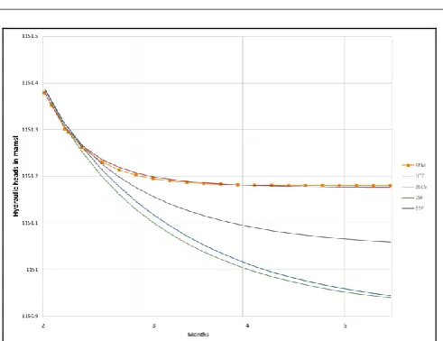
In Figure 1, the modelled and predicted groundwater elevation at observation well OBS_9 are shown for the four dewatering strategies as examples of the responses obtained. In this figure, the modelled (FEM) groundwater elevations, as well as the groundwater elevations predicted by four ANNs using different transfer functions, are plotted against the dates of measurement.
[image:3.595.312.558.66.255.2]It can be seen that the predictions of hydraulic heads made by the ANNs models generally underestimate the hydraulics heads from the numerical model. It can be also seen that ANN using the hyperbolic transfer function (HTF) yielded the best predictions of the modelled (FEM) hydraulic heads for three of the four dewatering scenarios (3, 6, 9 and 12 abstractions wells). It can furthermore be seen that the accuracy of the head predictions made by the ANNs generally decreased over time. However, for all observation points, the difference between the modelled and predicted hydraulic heads seldom exceeded 0.5 m.
Figure 1: Modelled and predicted hydraulic heads at observation well OBS_9 for a dewatering strategy using 12
dewatering wells
To verify the accuracy of the hydraulic head predictions, statistical techniques were used to assess the performance of the different ANNs. The performance analyses were carried by considering the modelled and predicted hydraulic heads at all nine observation points (OBS_1 to OBS_9) for all four dewatering simulations (using 3, 6, 9 and 12 abstraction wells).
In Figure -2, the Root Mean Square Errors (RMSEs) for the hydraulic head predictions made by the ANNs using the four different transfer functions are shown at all nine observation points. The RMSEs for the ANNs using the BSF, LSF, ZLBSF and HTF are shown in green, blue, brown and orange, respectively. From this figure it can be seen that the HTF yielded the smallest errors at most observation wells, followed by the BSF. The ANN using the ZLBSF and LSF gave the largest errors (poorest predictions). Similar observations can be made when considering the Normalised Root Mean Square Errors (NRMSEs) (refer to Figure -3).
Figure -4 shows the RSR calculated for the hydraulic head data at all the observation wells. From this figure, it is seen that the ANN using the HTF yielded the lowest RSR values at most observation wells, and therefore gave the best performance in predicting the hydraulic heads at the different piezometers.
In Figure -5 the PBIAS for the groundwater elevation data at all the observations wells is shown. Again the ANN with the HTF gives the lowest (closest to zero) values for the PBIAS at most observation wells. This ANN therefore performed the best in predicting the hydraulic heads.
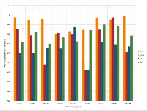
© 2017, IRJET | Impact Factor value: 6.171 | ISO 9001:2008 Certified Journal | Page 1417 r correlation coefficients therefore indicate that the ANN was
able to successfully predict changes in the hydraulic heads. At six of the nine observation wells, the ANN using the HTF had r-values closer to 1 than the ANNs using the other transfer functions. It can therefore be concluded that the ANN using the HTF performed better than the other ANNs in predicting the hydraulic heads at the observations wells.
From Figure -7, it is seen that large negative NSE-values were calculated at some of the observation wells for the predictions made by the ANNs using the ZLBSF, LSF and BSF. Positive or small negative NSF-values were calculated for the ANN using the HTF. This ANN therefore outperformed the others in its predictions of the hydraulic heads.
[image:4.595.315.556.66.245.2]From Figure -8 it can be seen that, at most wells, the lowest PI values were calculated for the ANN using the HTF. This transfer function therefore yielded the best results.
Figure -2: Root Mean Square Errors (RMSEs) for the hydraulic head predictions at the different observation
wells
Figure -3: Normalised Root Mean Square Error (NRMSE) for the hydraulic head predictions at the different
[image:4.595.314.553.285.459.2]observation wells
[image:4.595.43.281.292.460.2]Figure -4: RMSE-observations Standard deviation RATIO (RSR) for all observation points
Figure -5: Percent BIAS (PBIAS) for all observation points
Figure -6: Pearson correlation coefficient (r) for the hydraulic head predictions at the different observation
[image:4.595.312.555.491.675.2] [image:4.595.42.281.513.683.2]© 2017, IRJET | Impact Factor value: 6.171 | ISO 9001:2008 Certified Journal | Page 1418 Figure -7: Nash-Sutcliffe Efficiency (NSE) for the hydraulic
head predictions at the different observation wells
Figure -8: Performance Index (PI) for all observation points
4. GRAPHICAL MODEL EVALUATION TECHNIQUES
From the statistical evaluation techniques, the model based on the HTF was found to be most suitable to predict the groundwater elevations. In this section, graphical residual analysis will be used to further assess the performance of the ANN using this transfer function.
In Figure -9, the hydraulic heads predicted at OBS_9 by the ANN using the HTF are plotted against the modelled (FEM) hydraulic heads for the four dewatering scenarios (3, 6, 9 and 12 dewatering wells). From this figure, it can be seen that predicted values give good approximations of the modelled values. The R-squared values of the linear fits range between 0.91 and 0.99, indicating that hydraulics heads predicted by ANN fit the regression line well.
However, it is known that the R-squared value cannot determine if the hydraulics heads predicted by the ANN are biased. For this reason, normal probability plots and residual plots were constructed for the data at the different observation wells. There are several methods to test the normality of data distribution. For graphical analysis, the
common techniques are the quantile-quantile (Q-Q) probability plot and the normal probability plot. The Q-Q plot is a technique used to determine if the data used for the analysis are from populations with the same distribution. The normal probability plot helps to evaluate if the dataset follows a normal or Weibull distribution (Chambers et al., 1983). In the current study, normal probability plots were used. These plots are graphs showing the percentile of the normal distribution against the residual values.
The normality plot for observation well OBS_9 during the four dewatering strategies is presented in Figure -10. From this figures it can be observed that there are minor deviations from the straight line fit. It can therefore be concluded that the data are normally distributed, since that plot shows strong linear patterns with R-squared values close to 1. No significant outliers are observed in the data.
The comparison between the outputs from the ANN and the FEM revealed good agreement between these two datasets. However, further examination of the data by means of residual plots could reveal systematic differences between the two datasets. Graphical residual analysis is used in this research to verify the quality of the agreement between the modelled and predicted data to determine whether the ANN needs further refinement for linearization.
Residual plots are firstly used to determine if the data fits the linearity and homogeneity of the variance assumptions. The plots have to be randomly distributed if the variance is homogeneous. To meet the linearity requirement, the residuals have to be equally scattered above and below the x-axis of the plot.
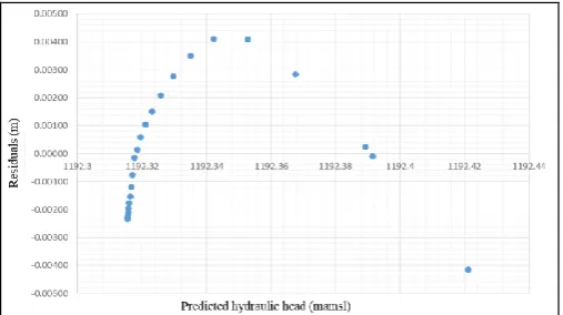
The residual plots of observation well OBS_9 is shown in Figure -11 for the four dewatering strategies. From that figure it is seen that the residual plots have non-random, inverted U-shaped patterns, suggesting that a better fit to the data could have been obtained using a non-linear model. The shapes of the residual plots suggest that the function used to describe data should be quadratic.
In an attempt to improve the predictions of the ANN, the ANN was refined by transformation of the data to achieve linearity. Transforming a dataset is to re-express it with another measurement scale using an appropriate mathematical operation. A non-linear transformation increases or decreases a linear relationship between variables, changing their correlation by so-doing.
[image:5.595.41.282.292.460.2]© 2017, IRJET | Impact Factor value: 6.171 | ISO 9001:2008 Certified Journal | Page 1419 Figure -9: ANN versus FEM hydraulic heads for
observation point OBS_9 using three dewatering wells
Figure -10: Normal probability plot for observation point OBS_9 using three dewatering wells
Figure -11: Residuals plots for observation point OBS_9 using three dewatering wells
7. DISCUSSION AND CONCLUSION
The main objective of this research was to use statistical methods to evaluate which transfer function used by the different ANNs results in the best prediction of the hydraulic heads obtained from the numerical model. ANNs using four different transfer functions were used and their performances were evaluated based on seven statistical evaluation techniques. The statistical evaluation results show that the ANN using the HTF best predicts the effects of the dewatering process at the open pit.
To simplify the concept, it is important to generate mathematical relation which can describe more easily the model. Then comes the need to use graphical techniques.
From the graphical residual analysis it is seen that there is a systematic non-linearity between the modelled and predicted datasets. Despite this non-linearity, all the other graphical evaluation techniques showed that the ANN was successful in predicting the hydraulic heads with high accuracy. For further researches, the developed ANN will be applied to a real open pit mine to predict the impact of dewatering strategies.
REFERENCES
[1] D. Moriasi, J. Arnold, M. Van Liew, R. Bingner, R. Harmel and T. Veith, “Model for evaluation guidelines for systematic quantification of accuracy in watershed simulations”, American Society of Agricultural and Biological Engineers, Vol. 50(3), 2007, pp. 885−900.
[2] H Gupta, S. Sorooshian and P. Yapo, “Status of automatic calibration for hydrologic models”, Journal of Hydrologic Engineering, Vol. 4 (2), 1999, pp 135 – 143.
[3] J. Cohen, J. and P. Cohen, “ Applied multiple regression - correlation analysis for the behavioral sciences”, Hillsdale, NJ: Lawrence Erlbaum Associates, Inc., 2017.
[4] J. Nash and J. Sutcliffe, “River flow forecasting through conceptual model, Part I – A discussion of principles”, Journal of hydrology, Vol 10, 1970, pp. 282 – 290.
[5] J. Osborne and E. Waters, “Four assumptions of multiple regression that researches should always test, Pratical assessment”, Research and Evaluation, Vol. 8 (2), 2002.
[6] J. Singh, H. Knapp and M. Demissie, “Hydrologic modeling of the Iroquois River watershed using HSPF and SWAT”, Journal of American Water Resources Association, Vol. 41 (2), 2005, pp 361 – 375.
[7] N. Sage, A. Mbuyu, J. Kabulo and A. Kalau, “ Implementation of a Finite Element Model to generate synthetic data for open pit’s dewatering”, IRJET, Vol. 4 (12), 2017.
[8] N. Sage, J. Lunda, A. Mbuyu and J. Kabulo, “Application of synthetic observations to develop an Artificial Neural Network for mine dewatering”, IRJET, Vol. 4 (12), 2017.
[9] N. Sage, “Development of artificial neural network for mine dewatering”, PhD thesis, University of the Free State, 200p., 2017.
[image:6.595.36.288.263.401.2] [image:6.595.36.290.446.588.2]© 2017, IRJET | Impact Factor value: 6.171 | ISO 9001:2008 Certified Journal | Page 1420 BIOGRAPHIE