Efficient Bayesian inference for partially observed stochastic epidemics and a new class of semi parametric time series models

(1)

Efficient Bayesian Inference for

Partially Observed Stochastic

Epidemics

and

A New Class of Semi

₋

Parametric

Time Series Models

Theodore Kypraios, MSc.

Submitted for the degree of Doctor of Philosophy

at Lancaster University,

(2)

Efficient Bayesian Inference for Partially Observed Stochastic Epidemics and A New class of Semi−Parametric Time Series Models

Theodore Kypraios, MSc.

Submitted for the degree of Doctor of Philosophy

at Lancaster University,

June 2007.

Abstract

This thesis is divided in two distinct parts. In the first part we are concerned

with developing new statistical methodology for drawing Bayesian inference for

partially observed stochastic epidemic models. In the second part, we develop a

novel methodology for constructing a wide class of semi−parametric time series models.

First, we introduce a general framework for the heterogeneously mixing

stochas-tic epidemic models (HMSE) and we also review some of the existing methods of

statistical inference for epidemic models. The performance of a variety of centered

Markov Chain Monte Carlo (MCMC) algorithms is studied. It is found that as

the number of infected individuals increases, then the performance of these

al-gorithms deteriorates. We then develop a variety of centered, non−centered and partially non₋centered reparameterisations. We show that partially non₋centered reparameterisations often offer more efficient MCMC algorithms than the centered

ones.

The methodology developed for drawing efficiently Bayesian inference for HMSE

is then applied to the 2001 UK Foot-and-Mouth disease outbreak in Cumbria.

Unlike other existing modelling approaches, we model stochastically the infectious

(3)

unknown. Due to the high dimensionality of the problem, standard MCMC

algo-rithms are inefficient. Therefore, a partially non−centered algorithm is applied for the purpose of obtaining reliable estimates for the model’s parameter of interest.

In addition, we discuss similarities and differences of our findings in comparison

to other results in the literature.

The main purpose of the second part of this thesis, is to develop a novel class of

semi−parametric time series models. We are interested in constructing models for which we can specify in advance the marginal distribution of the observations and

then build the dependence structure of the observations around them. First, we

review current work concerning modelling time series with fixed non₋Gaussian margins and various correlation structures. Then, we introduce a stochastic

pro-cess which we term a latent branching tree (LBT). The LBT enables us to allow for

a rich variety of correlation structures. Apart from discussing in detail the tree’s

properties, we also show how Bayesian inference can be carried out via MCMC

methods. Various MCMC strategies are discussed including non−centered param-eterisations. It is found that non−centered algorithms significantly improve the mixing of some of the algorithms based on centered reparameterisations. Finally,

we present an application of this class of models to a real dataset on genome

(4)

Acknowledgments

I feel extremely lucky that I met Petros Dellaportas during my undergraduate

studies in Athens University of Economic and Business. Apart from being a great

teacher, Petros was the first person who advised me to do a PhD and in particular

to come to the UK and be supervised by Gareth Roberts. I will always be grateful

to Petros for this suggestion and his valuable guidance all these years.

Working with Gareth has been really exciting. Apart from his energy and his

enthusiasm for research, his support and guidance throughout my PhD have been

invaluable. I very much enjoyed discussions on the intuition behind the work in

this thesis and many other subjects. I am grateful to Gareth for trying hard and

succeeding in a finding me a scholarship without which I would not be able to study

for a PhD. Gareth has been encouraging and very patient while I was writing up

this thesis and provided me with very constructive comments. After 4 years now,

I believe that I made a very good friend. For all these and many more I would like

to thank him.

It has been a great pleasure that I had the chance to study in Lancaster where I

had the chance to exchange ideas and collaborate with many interesting people.

In particular, I would like to thank Paul Fearnhead for his support and guidance

through my PhD. I am also grateful to him for many interesting discussions and

for providing me the genome scheme data used in the second part of this thesis.

Furthermore, I feel very lucky that coming to the UK, the first person I met

was Omiros Papaspiliopoulos. Apart from being a very good friend, Omiros has

(5)

been very supportive and his help during my PhD has been very important. I

would also like to thank my friends Alexandros Beskos, Kostas Kalogeropoulos

and Nikos Demiris for many fruitful discussions. Pete Neal and Chris Jewell have

been exciting collaborators and I am very happy that I had the chance to work

with them.

In addition, many other people made my time in Lancaster enjoyable. I would

particularly like to mention my officemates Jamie Kirkham, Chris Sherlock, Mark

Latham and Rosemeire Fiaccone for suffering silently when half of the Greek

com-munity in Lancaster was visiting me in the office. Furthermore, I would like to

mention the friends of mine who I played music with (Dimitris, Kostas, Kostas

and Manolis) and those who have suffered listening to us (too many to mentioned

here). Also, a big thank to my flatmates throughout the years I spent on campus:

Alexandra, Vanessa, Dina, Nik and George - I will never forget the moments we

shared together. Although there are people out there who sharing the time with

has been very rewarding, there are too many to be mentioned here. My special

thanks to Anastasia Lykou for printing for me the final version of this thesis!

I would also like to thank Omiros Papaspiliopoulos, Paul Fearnhead, Simon

Pre-ston, Pete Neal and Chris Jewell for useful comments on earlier versions of this

thesis. I would also like to thank Thomas Miles in DEFRA who provided us for

the data on 2001 UK Foot-and-Mouth disease outbreak.

Last but not least, my family was extremely supportive throughout this period,

despite me being abroad - many thanks to them. Since my my very best friends

from Rhodes (Thanasis, Leandros, Mixalis and Stefanos) also considered as

’fam-ily’, they also deserve to be thanked for their patience and support for all the years

we know each other.

Finally, I would like to thank Lancaster University for its financial support during

(6)

Declaration

I hereby declare that this thesis is my own work, except otherwise stated, and has

not been submitted in substantially the same form for the award of a higher degree

elsewhere.

The computationally intensive algorithms in Chapters 2, 3 and 5 were coded in

the C programming language and used the GNU Scientific Library for generating

random variables. All other computational work in this thesis was carried out in

the R statistical environment. All computer code included in this thesis was my

own.

Theodore Kypraios

(7)

(8)

List of Tables

2.1 Nomenclature for the centered MCMC algorithms . . . 79

2.2 Nomenclature for the centered reparameterized MCMC algorithms . 85

2.3 Nomenclature for the PNC algorithms . . . 92

2.4 Nomenclature for the EPNC MCMC algorithms . . . 98

2.5 Three simulated datasets with different infectious period . . . 101

2.6 Estimates of the integrated autocorrelation function of the

param-eter γ using the 10% deterministic scan centered algorithms for datasets D1, D2, D3 . . . 107

2.7 Estimates of the integrated autocorrelation function of γ using the

centered reparameterised algorithms for datasets D1, D2, D3 . . . . 115

2.8 Estimates of the integrated autocorrelation time of the parameter

γ for the different PNC and EPNC algorithms . . . 118

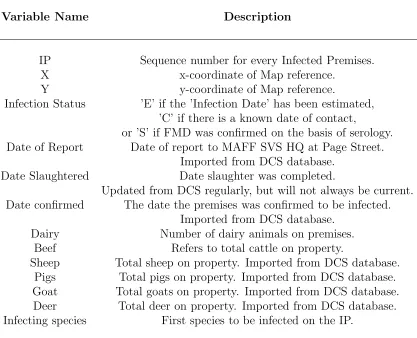
3.1 Information on the infected premises . . . 150

3.2 Summary statistics for the number of cattle and sheep of each farm

in Cumbria . . . 155

3.3 The form of the different kernels used for the 2001 UK FMD outbreak163

3.4 Parameter estimates and approximate 95% highest posterior density

region for model’s parameters . . . 167

(9)

5.1 A variety of transformations of a standardized Normal VariableX ∼

N(0,1) . . . 193

(10)

List of Figures

1.1 The graphical model of the centered reparameterisation . . . 22

1.2 The graphical model of the non₋ centered reparameterisation . . . 22 1.3 A path in [0,1] of a standard Brownian motion. It has been

simu-lated by discretising time in intervals of length 0.001 and simulating

from the corresponding increments of the process . . . 24

2.1 The three transition states of an individual. . . 40

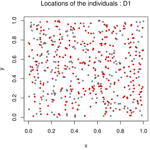
2.2 The locations of the 501 susceptibles individuals. Red dots denote

the infected individuals of the dataset D1. . . 101

2.3 The distributions of the infectious periods for the simulated data

sets 1 (black), 2 (red), 3 (green). . . 102

2.4 ACFs for the average infection time I using random scan (top left),

10%, 50% and 100% deterministic scan update (top right, bottom

left and right, respectively) applying the standard [C] algorithm to

dataset 1. . . 106

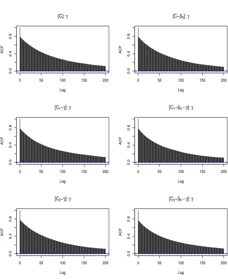
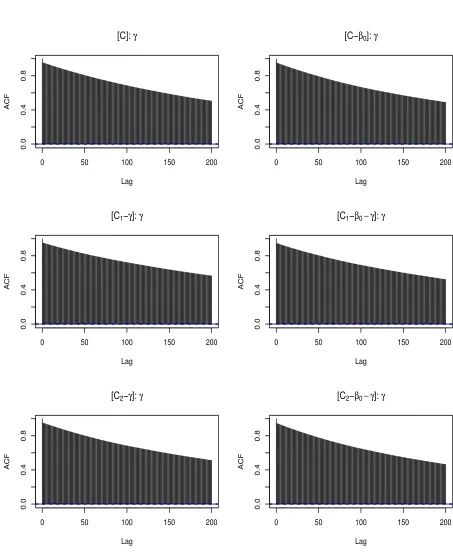
2.5 ACFs of parameter γ, using the centered algorithms presented in

Table 2.1 for dataset D1. . . 108

(11)

2.8 ACFs of the parameter ψ =β0/γ, using samples of the parameters

β0 and γ, obtained from the [C] algorithm (see Table 2.1). Each

ACF refers to the different datasets (see Table 2.5). . . 111

2.9 Scatter plot between γ and I obtained from their posterior samples

using the [C] algorithm for each of the three different datasets. . . 113

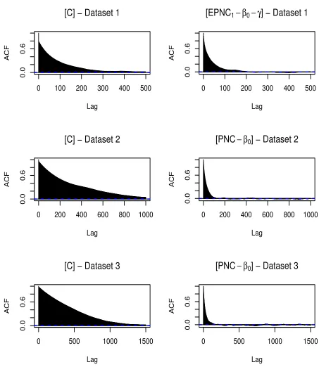
2.10 Comparison of ACFs of γ between the centered and the optimal

PNC algorithm for the different datasets. Details on the

nomencla-ture of the algorithms are given in Tables 2.3 and 2.4 . . . 119

3.1 The spatial distribution of susceptible farms in the UK at the start

of the outbreak (green) and of the infected farms at the end of the

outbreak (red). . . 152

3.2 The spatial distribution of susceptible farms in Cumbria at the start

of the outbreak (green) and of the infected farms at the end of the

outbreak (red). . . 153

3.3 Histograms of the number of cattle and sheep for the all the

suscep-tible farms in Cumbria . . . 154

3.4 Different distributions for the infectious period given specific values

of the shape and the scale parameter . . . 157

3.5 Posterior distribution of parameter γ (left) and the corresponding

mean infectious period (right) . . . 161

3.6 A 95% highest posterior density region of K(i, j). The black line

refers to the “average” shape of the Kernel, based on the posterior

mean of π(δ_|R) . . . 162 3.7 The relative kernel’s effect for the Cauchy-, geometric- and

(12)

3.8 Posterior distributions of the model parameters. Red line shows the

prior distributions. . . 166

3.9 Average posterior farm’s infectivity under the number of cattle

(green) and sheep (red), T = nζ

c and T = nζs respectively (top) and susceptibility, S =ξnζ

c and S =nζs respectively (bottom). . . . 168

4.1 The four compartments of the SINR model. . . 180

5.1 A series 3,000 observations collected over time. . . 188

5.2 Histogram (left) and ACF plot for the data shown in Figure 5.1(right).188

5.3 Generation of four real data points (Y1, Y2, Y3, Y4) where the ”jump

distribution” is Uniform[0,1]. (see the text for more details) . . . . 192 5.4 Rate of decay of the covariance, O(·) . . . 198 5.5 Density plots of the Beta distributions (left) and ACF plots for the

realizations (right). . . 200

5.6 The first 5,000 realizations obtained via a LBT using Beta(1,20)

(top) and Beta(20,1) (bottom) as “jump distributions” . . . 201 5.7 An LBT construction using a mixture of Beta distributions as“jump

distribution” . . . 202 5.8 A Skeleton of a LBT . . . 205

5.9 Graphical model of the centered (top) and and non₋centered hier-archical parameterisation of the model . . . 218

5.10 ECDF of times for the Uniform“jump distribution”- Red line shows the true CDF . . . 224

5.11 Posterior distributions of the divergence times τ20, τ22, τ12 . . . 226

(13)

5.13 ECDF of times for the Fr´echet“jump distribution” - Red line shows the true CDF . . . 228

5.14 ACF of the average divergence time point - JD: Fr´echet . . . 229

5.15 Posterior distribution of α obtained via the Centered MCMC

algo-rithm . . . 233

5.16 ECDF of times for the Beta(α,1) “jump distribution” - Red line shows the true CDF . . . 234

5.17 ACF plot of the posterior sample obtained via the centered

algo-rithm . . . 235

5.18 Correlation plot between missing data and model parameter . . . . 236

5.19 Centered (top) and Non−Centered Parameterisations . . . 236 5.20 ACF plot of the posterior sample obtained via the non₋centered

algorithm . . . 240

5.21 Number of C+Gs included in each window of 3,000 from the DNA

sequence . . . 243

5.22 ACF and PACF plot of the normalised data . . . 243

5.23 Histogram of the non-normalised (left) and normalised (right) data.

Red lines reveals the Normal curve. . . 244

5.24 ACF plots for two subsets of the data . . . 244

5.25 ACF plot of the data. The green line indicates the rate of decay of

the covariance function according to an assumed Fr´echet distribution245

5.26 Posterior distribution for the 4thdivergence time points assuming a Uniform (top) and a Fr´echet (bottom) prior for the vector τ. . . 250 5.27 Posterior distribution for the 5thdivergence time points assuming a

(14)

5.28 Posterior distribution for the 6thdivergence time points assuming a

Uniform (top) and a Fr´echet (bottom) prior for the vector τ. . . 252 5.29 A simulate realisation from the fitted model using the posterior

mean of the divergence times . . . 253

5.30 Smoothed Spectrum and PACF plots of 1,000 realisations of the

fitted model using samples from the posterior distribution of the

divergence time points τ. The blue line is obtained by simulating a realisation of the model using the posterior means the posterior

distributions. The green line refers to the plots obtained from the

actual real data. . . 254

(15)

Chapter 1 Introduction

1.1 Motivation

During the last two decades, sampling-based methods for performing Bayesian

inference have been widespread. The need for considering realistic models to

adequately explain particular phenomena has lead to inferential problems which

involve multidimensional analytically intractable integrations. However, such

in-tegrations can be easily managed by using Monte Carlo methods which are

par-ticularly appropriate within this framework, (see for example, Smith and Roberts,

1993). Suppose, we have a probability density π(x), corresponding to some

ran-dom variable, X and a function f of interest. It is often the case that we might

be interested in evaluating integrals of the following form:

Eπ(f) =

Z

x

f(x)π(x) dx (1.1)

Suppose thatπ(x) is multidimensional and analytical calculations are impossible.

However, we are able to draw a sequence of values,Xi, such thatXi are identically and independently distributed (i.i.d.) with density π. Then it is true that

E

"

1

n

X

i=1 f(Xi)

#

=Eπ(f) (1.2)

(24)

and by the strong law of large numbers if we take n to be large enough we could approximate the desired expectation by:

1

n

X

i=1

f(Xi)≈Eπ(f) (1.3)

Furthermore, we might also use the Central Limit Theorem (CLT), given that π

admits a variance for the function f(x), say σ2_{, to see how accurate this estimate}

might be:

1

n

Pn

i=1(f(Xi)−Eπ(f))

σ√n ∼N(0,1) (1.4)

Therefore, the computational challenge which has to be faced is how to draw

sam-ples fromπwhich will be used in (1.3). Techniques which attempt to draw directly

from π(x) have been shown to have limited applicability. Instead, a large

collec-tion of powerful, iterative computacollec-tional algorithms which are general and easy

to implement, have found a great success within the statistical community since

early 1990s. These methods are known as Markov Chain Monte Carlo (MCMC) and the main idea goes back to 1953 in the particle Physics literature (Metropolis

et al., 1953). Then it was generalised in statistical context by Hastings (1970).

Nevertheless it is much later with Gelfand and Smith (1990) that the statistical

community became aware of the potential of MCMC for Bayesian inference. Since

then, the use of Bayesian methods for applied statistical modelling has increased

rapidly.

MCMC methods enable us to draw a sequence Xn, n = 1,2, . . ., which although neither independent nor identically distributed, still satisfies (1.3). The idea behind

MCMC is the following: for a given distribution π, on an arbitrary state space X, construct a Markov chain with the same state space and stationary distributionπ.

(25)

distributional convergence of the realisations, i.e.

Xn d →π

where→d denotes the convergence in distribution. In addition, they ensure consis-tency of “ergodic averages”, for any integrable scalar function f,

1

n

X

i=1

f(Xi)→

Z

X

f(x)π(x) dx, asn_{→ ∞}, almost surely

The dependence among the simulated values plays a very significant role in terms

of the efficiency of an MCMC algorithm. The “ergodic averages” such as in (1.3)

can become very unstable and converge very slowly to their strong limited values

in the presence of very high serial correlation in the_{Xn}series.

Therefore, the motivation behind this thesis is to provide a general methodology

for constructing efficient MCMC algorithms so as to reduce the serial dependence

and obtain more reliable results.

1.2 Structure of the Thesis

This thesis is divided into two discrete parts. The first part is mainly concerned

with drawing Bayesian inference for stochastic epidemic models. The focus is

to construct and analyse a class of non−centered parameterisations which can improve the speed of the convergence of the Gibbs sampler (see Section 1.6.1

for definition) and other related MCMC algorithms. This part consists of three

chapters and which are outlined below.

• Chapter 2. In this chapter, we will first explain why understanding the spread of an infectious disease is an important issue in order to prevent major

outbreaks. We will also provide a historical background on deterministic and

(26)

briefly review the previous work in epidemic modelling by mainly focusing

on the general stochastic epidemic model and describing existing approaches

for drawing classical (frequentist) and Bayesian inference for its associated

parameters.

Furthermore, we introduce a more general and realistic model to capture the

dynamics of infectious diseases. We will demonstrate how standard methods

can be applied for inferential purposes and also show via an illustrative

ex-ample that they can be problematic in some cases. Therefore, we will mainly

focus how to develop a class of centered and non₋centered reparameterisa-tions in order to obtain more robust and efficient algorithms.

• Chapter 3. This chapter is mainly concerned with modelling the 2001 UK Foot-and-Mouth (FMD) outbreak from a fully Bayesian perspective. First,

we will refer to the previous work on modelling the FMD outbreak and then

adopting the methodology presented in Chapter 2 we will focus on describing

the transmission’s dynamics of the disease. Moreover, we will compare our

findings with those presented in the literature already.

• Chapter 4. In the final chapter of Part I, we discuss various extensions of methods and applications for partially observed stochastic epidemics. This

chapter also includes a first attempt to provide a real-time risk assessment

tool for a potential Avian Influenza outbreak in the poultry industry of the

UK.

In the second part of the thesis we introduce a wide class of semi₋parametric time series models based on an underlying stochastic process, which we term la-tent branching tree. The motivation behind this chapter is to develop a general methodology to construct time series with pre-specified marginal distributions of

the observations and build the correlation structure around them. The structure

(27)

• Sections 5.1, 5.2, 5.3. In the beginning of this chapter we will briefly review the literature on constructing time series models with fixed margins

outside the Gaussian context with a specific correlation structure. Then, we

present some motivating examples of time series that we will be interested

in modelling via our class of models.

• Sections 5.4, 5.5, and 5.6. In these sections, the construction of a latent branching tree based on diffusions is given and the general properties of the

tree are discussed. We will refer to the nature of realisations obtained via

the proposed stochastic process by focusing on their marginal distribution

and their corresponding dependence structure.

• Sections 5.7 and 5.8. We show how we can simulate a latent branching tree

exactly without the need of discretisation of the diffusions processes which are chosen to build the tree. We demonstrate how Bayesian inference can

be conducted for the parameters of interest via MCMC methods. Moreover,

we describe in detail alternative MCMC strategies, including non−centered parameterisations, so as to improve the efficiency of the standard algorithms.

• Sections 5.10 and 5.11. In these sections we first present a simulation study to illustrate the performance of the proposed class of models. Then

we apply our methodology to analyse some real genome scheme data.

• Sections 5.13 and 5.12. Finally, we summarize the advantages of the proposed methodology and also discuss further extensions regarding

gener-alisations of the existing methods and also extensions which are motivated

by real applications.

1.3 Bayesian Inference

In this section we will describe the fundamentals of Bayesian inference. A rigorous

(28)

1.3.1 Bayes’ Theorem

Bayesian inference, similarly to likelihood inference, requires a sampling model

that produces thelikelihood, the conditional distribution of the data given the pa-rameters. Then, the Bayesian approach will additionally place apriordistribution on the model parameters. The likelihood and the prior are then combined using

Bayes theorem to derive the posterior distribution. The posterior distribution is the conditional distribution of the (unknown) parameters, denoted byθ given the data, denoted byY. All Bayesian inference arises from the posterior distribution. Adopting a Bayesian approach, a prior distribution is assigned to θ and we are interested in deriving explicitly or sampling from the posterior distribution of θ,

π(θ_|Y). In the case of a continuous state space, the posterior turns out to be:

π(θ_|Y) = R π(θ)L(Y|θ) θπ(θ)L(Y|θ) dθ

(1.5)

We refer to this formula as the Bayes’theorem. The integral in the denominator is essentially a normalising constant and its calculation has traditionally been a

severe obstacle in Bayesian computation. In Section 1.6, we will demonstrate how

we can avoid its calculation using MCMC methods. In terms of a discrete state

space the integral is substituted with a sum over the sample space of θ. In this

thesis we are mainly concerned with continuous state spaces and therefore in the

rest of this chapter we omit the corresponding results for the discrete state spaces.

Bayes’ theorem can be used sequentially. Suppose that we have collected two

independent data samples,Y1 and Y2.

π(θ_|Y1,Y2) ∝ L(Y1,Y2|θ)π(θ)

∝ L(Y2|θ)×L(Y1|θ)×π(θ)

∝ L(Y₂_|θ)_×π(θ_|Y₁)

(29)

dataset by first evaluating π(θ_|Y1) and then treating it as a prior for the second

datasetY2. Thus, we have a natural setting when the data arrive sequentially over

time.

1.3.2 Priors

The choice of the prior distribution has drawn a considerable attention in the

Bayesian community (see for example, Bernardo and Smith, 1994). In this section

we briefly present some of the most popular approaches for choosing the priors.

Additionally to the priors we mention here there exist the so called elicited priors,

created using an experts opinion. However, elicitation methods go beyond the

scope of this thesis and we shall not give more details here.

It is possible to select a distribution which is conjugate to the likelihood, that is, one that leads to a posterior belonging to the same family as the prior. Morris

(1983) showed that exponential families, where likelihood functions often belong,

do in fact have conjugate priors, so that this approach will typically be available in

practice. The great advantage of such a prior is that can be more computationally

convenient than others.

In many practical situations prior information aboutθ is not available. Therefore, the need of specifying non-informative priors is essential. In other words, we would like to define a prior distributionπ(θ) that contains very little information about the parameter of interest,θand argue that the information contained in the posterior about it, comes almost entirely from the data. Summarizing, we should

always choose a prior for the parameter of interest very carefully.

1.3.3 Posterior Distribution

Having obtained the posterior distribution for the parameters of interest we have

all the information that the data contain for the parameters. A natural first step

(30)

addition, we can obtain summaries of our posteriors which can give us all the

information that can be obtained using a frequentist approach to inference. In

this section we will mention the most commonly used in practice, point estimation

and interval estimation.

Point estimation is readily available through π(θ_|Y). The most commonly used location measures are the mean, the median and the mode of the posterior

distri-bution since they all have appealing properties. Depending on the shape of the

posterior distribution one of the aforementioned measures can be used.

In the case of a continuous parameter space Θ, a 100_×(1₋α)% credibility set forθ is a subset of Θ which satisfies the following:

1−α≤P(C|Y) =

Z

C

π(θ_|Y) dθ (1.6)

where integration is replaced by summation for discrete components of the

param-eter.

One of the most attractive credibility sets, is the highest posterior density region

defined as:

C =_{θ _∈Θ:π(θ_|Y)_≥q(α)_} (1.7) whereq(α) is the largest constant satisfying π(C_|Y)_≥1₋α. This credibility set consists of the most likely θ values. Nevertheless, it can be hard to compute such integrals analytically and therefore numerical methods should be applied. On the

other hand, a much easier and commonly used approach is to calculate the equal

tail credibility set by simply taking the α/2− and 1−α/2− quantiles of π(θ_|Y) which equals to the highest posterior density set for symmetric unimodal densities.

(31)

1.4 Bayesian Inference for Missing Data

Prob-lems

LetY denote the observed data,X the missing data andθ the parameters in the model. The statistical models considered in this thesis share a common structure:

the distribution of (Y,X) is specified and depends on the parameter θ. Never-theless, only Y is observed, and therefore X is treated as missing data. The pair of (X,Y) is often known as the augmented or complete data. The term “missing data” can either be interpreted as data which for some reason we failed to collect

or data which are not available to us. On the other hand, in many cases, especially

in models with latent variables, random effects, or hidden stochastic processes, we

would never be able to observe X.

By adopting a Bayesian approach, the conditional distribution of the parameter

(in a continuous state space) given the observed data is given up to proportionality

as follows:

π(θ_|Y)∝π(θ)

Z

X

π(Y,X_|θ) dX (1.8) This means that in order to perform posterior inference for θ we need to find the marginal distribution of the observed data given the parameters. In practice,

in many complex statistical models used nowadays, for example in econometrics,

geostatistics and engineering, the integralR_Xπ(Y,X_|θ) dXis neither analytically or numerically feasible.

Nevertheless, powerful iterative sampling schemes have been developed which

(32)

and Roberts (1993).

1.5 Conditional Independence

We say that two variablesX and θare independent, and we writeX_⊥θ, when any information received for θ does not alter uncertainty about X, see Dawid (1979):

π(X|θ) = π(X)

The concept of conditional independence is very important in this thesis. The

centered and the non₋centered parameterisations which are introduced in 2 and 5 are defined in terms of the conditional independence structure they impose between

the missing data and the parameters.

Following Dawid (1979) who develops the theory of conditional independence in

the statistical context, the random variables Y and θ are said to be conditionally

independent given another variable X, when they are independent in their joint

distribution conditional onX =x, for any value of x. That is

π(Y, θ_|X) =π(Y_|X)π(θ_|X).

Marginally though, when X is unknown Y andθ could be dependent. The

condi-tional independence is often expressed in terms of factorisation of the joint density

ofX, Y, θ. A compact and illustrative way of expressing conditional independence

statements is by means of graphical models and such an approach is often adopted

(33)

1.6 Markov Chain Monte Carlo Methods

Markov chain Monte Carlo methods are employed to (approximately) draw samples

from a specific distribution π say, which is often called as target distribution. π

is typically multidimensional and in the application we will be concerned in this

thesis, is the joint posterior distribution of the parameters and the missing data

in a hierarchical model.

In this section we will present the main idea and review some well known MCMC

algorithms. There is a vast literature about the theory, methodology,

implementa-tion and applicaimplementa-tions of MCMC. Currently available texts on the subject include,

for, example Gilks et al. (1996), Tanner (1996), Robert and Casella (1999) and

Roberts and Tweedie (2006).

We shall briefly describe some of the MCMC algorithms most relevant for our

purposes. For more details, we refer to the aforementioned books for details. The

main idea behind MCMC methods has already been mentioned; for a given target

distributionπ, MCMC methods construct a Markov chain{Xn}which hasπas an invariant measure. Mild conditions ensure that π is also a limiting distribution of

the chain, whatever the initial value X0. Such Markov chains, are called ergodic.

Most of the MCMC algorithms used in practice satisfy the condition which ensure

convergence to the invariant distribution π. An essential task in designing an

MCMC algorithm is to ensure that π is invariant which is mostly achieved using

the idea of reversibility.

From a statistical perspective, the convergence in distribution of the Markov chain

to π is exploited to estimate expectations under the invariant measure. More

details about convergence results can be found in Roberts and Tweedie (Chapter

8, 2006). In Bayesian analysis, π is a posterior distribution and most inference

problems come down to calculating expectations, (see for example, Gelfand and

Smith, 1990). Therefore MCMC is a very powerful tool for posterior inference,

(34)

Having ensured the convergence to stationarity, the question which is of interest, is

the speed at which an MCMC algorithms converges. This practically determines

how much time we should “run” the chain before the simulated values are assumed

to be drawn from π. A related concern is the dependence among the simulated

values. Even if we start at stationarity by sampling X0 ∼ π, the Markov chain

will generate exact but dependent samples from π. High dependence among the

sample can often lead in very slow convergence of the ergodic average estimates

to the expectations under π. The effect of the dependence among the sample is

discussed in more detail in Section 1.10.

1.6.1 Gibbs Sampler

The Gibbs sampler decomposes the state space _X as X1 _{× X}2 × · · · Xk, k > 2 and simplifies a complicated multi-dimensional simulation into a collection of k

smaller dimensional which are often more manageable. Often, _X = Rd_, _X

i =Rri and P_iri = d. The factorisation of the space is usually naturally suggested by the statical model which is considered. We adopt the following notation; we write

x= (x(1)_{, . . . , x}(k)_{) for an element of}_X _{where denote by}_x(i) _{∈ Xi, for all 1}_≤_i_≤_k_.

Also denote by x(−i) for the vector produced by excluding theith component from the vectorx.

x(−i) = x(1), . . . , x(i−1), x(i+1), . . . , x(k)

We also follow the same notational conventions for the random variable X _∼ π. The conditional distribution X(i)_|_X(−i) ₌_x(−i) _{for all} _i_{= 1}_{, . . . , k} _{is denote by}

πi ·|x(−i)

.

(35)

The Deterministic Scan Gibbs Sampler

1. Choose X0;

2. Set n = 0;

3. Repeat the following steps:

Set i= 1;

While i < k+ 1

{

Sample X_n(i₊₁) _∼πi ·|x(−i), where

x(−i) =X_n(1)₊₁, . . . , X_n(i₊₁−1), X_n(i+1), . . . , X_n(k)

i=i+ 1

}

n =n+ 1

The above scheme is also referred to as thedeterministic scan (DS) Gibbs sampler because of the way the algorithms visits each of the k components. It creates a

Markov chain onX with transition kernelP which is the composition ofk kernels,

P(i)_, _i_{= 1}_{, . . . , k}_{. In particular, if} _{z, w} _{∈ X} _{we define}

P(i)(z, dw) =

          

πi dw(i)|x(−i)

, for w(−i)₌_x(−i)

0, otherwise

(36)

Therandom scan (RS) Gibbs sampler at each iteration chooses one of the k com-ponents to update. Therefore its transition kernel can be written as

PRS =

P(1)₊_{· · ·}₊_P(k)

k .

The RS Gibbs sampler can be implemented as follows:

The Random Scan Gibbs Sampler

1. Choose X0;

2. Set n = 0;

Sample I from U(_{1,2, . . . , k_});

Sample X_n(I₊₁) _∼πi ·|x(−I)

Set X_n(j₊₁) =Xn(j), for j 6=I;

n =n+ 1

It can be checked that each P(i) _{is reversible with respect to} _π_{, from which easily}

follows thatπinvariant for either the composition, as in the DS or the mixture as in

the RS Gibbs sampler of theP(i)_{’s; see for example Theorem 3.4.2 and Proposition}

3.3.3. of Roberts and Tweedie (2006).

Apart from the RS and DS, there exist some other variation of the Gibbs sampler;

the random permutation Gibbs sampler chooses at each iteration a permutation of the components, and updates the components according to that permutation.

Note that this preserves reversibility. Another natural way to make the Gibbs

sampler reversible is to carry out two iterations of the Gibbs sampler, the second

one being implemented with the order of the other components reversed. Note that

(37)

end of the first iteration and the beginning of the second. The resulting algorithm

is called reversible Gibbs sampler. The implementation of this kind of the latter algorithms is straightforward; see for example Roberts and Tweedie (Section 2.2.2,

2006).

1.6.2 The Two-Component Gibbs Sampler (Data

Augmen-tation)

The data augmentation was originally developed by Tanner and Wong (1987) for

finding fixed point solutions to integral equations which appear in statistical

in-ference and it can be viewed as the stochastic analogue to EM algorithm (see

Dempster et al., 1977). It is most often used to obtain samples from the joint

dis-tribution ofX = X(1)_{, X}(2) _{say, by sampling from the conditional distributions.}

Such a scheme has a similar structure with the Gibbs sampler with Gelfand and

Smith (1990) showing that the latter is at least as efficient as the former.

Follow-ing the standard practice in the literature (see for example, Liu et al., 1994, Meng

and van Dyk, 2001), we will identify in this thesis the data augmentation with the

two-component Gibbs sampler.

Data augmentation is by far the most widely adopted computational method for

performing modern Bayesian analysis of missing data problems. The target

distri-bution is the joint posterior of the missing dataX and the parametersθ. By con-struction, simulation from the conditional distributionsπ(θ_|X, Y) andπ(X_|θ,Y) are tractable and more feasible than simulation from the marginal distribution of

the parameters given the observed data, π(θ_|Y). Note that there are many cases where the latter is not even available in closed form due to the integration in (1.5).

(38)

1.6.3 The Metropolis-Hastings Algorithm

The Metropolis algorithm (Metropolis et al., 1953) manages to sampleπ, at least

approximately, in a way which does not require the knowledge of its normalisation

constant. In this section we will describe the more general Metropolis−Hastings algorithm introduced by Hastings (1970). It is generally believed that most of

the MCMC algorithms can be considered as a special case of this algorithm. We

denote byπu the un-normalised density on Rd with respect to d-Lebegue measure,

µLeb

d . Also assume that is possible to carry out simulations of a Markov chain with transition density q(X,_·) with respect to the same measure. Such a transition density, called proposal density does not need to have any connection with πu, although its choice is important since it can actually influence the efficiency of the

resultant Markov chain.

The Metropolis-Hastings algorithms proceeds as follows. An initial starting value

X0 is chosen; then given the current state of the chain, Xn=x, a candidate value

Yn+1 =y is generated according to the proposal density q(Xn,·). The generated values is then accepted with probabilityα(x, y) , given by:

α(x, y) =

    

minπu(y)

πu(x)

q(y,x)

q(x,y),1

, if πu(x)q(x, y)>0 0, if πu(x)q(x, y) = 0

If the candidate value is accepted, then we set Xn+1 = y, otherwise if it is not

accepted, we set Xn+1 =x. It easy to see that the Markov chain induced by such

an algorithm has transition law P with densities

p(x, y) =q(x, y)α(x, y), x₆=y

with respect to µLeb

d and with probability of remaining at the same value equal to

r(x) =

Z

(39)

The algorithm is implemented as follows:

The Metropolis Hastings Algorithm

1. Choose X0;

2. Set n = 0;

Sample Yn+1 ∼q(Xn,·);

Sample Un+1 ∼U(0,1); If Un+1 ≤α(Xn, Yn+1) then

Set Xn+1=Yn+1;

Else

Set Xn+1=Xn;

n =n+ 1

It can be easily proven (see for example, the Lemma 2.4.1. of Roberts and Tweedie,

2006) that the algorithm ensures reversibility of the chain with respect to π, i.e.

satisfies the detailed balance

π(x)p(x, y) = p(y)p(y, x).

We should note that any α(_·,_·) which satisfies the following equation

π(x)q(x, y)α(x, y) =π(y)q(y, x)α(y, x)

can be used. A class of algorithms which have other accept/reject rules can

be found in Peskun (1973). However, it turns out that the accept/rule of the

(40)

moves. Therefore, it is also optimal in the sense of minimising the asymptotic

variance of any ergodic average moment estimator (see for example Peskun, 1973,

Tierney, 1998, Roberts and Tweedie, 2006).

The framework of the Metropolis-Hastings algorithm is very general since it does

not impose any restriction on the choice of q(_·,_·). Therefore, we will proceed by describing some special cases of this algorithm which have draw much attention in

the literature. The simplest possible choice of for the proposal distribution chooses

q(·,·) to be independent of its first argument:

q(x, y) =q(y)

and therefore we can write the accept/reject ratio as

α(x, y) = min

πu(y)

πu(x)

q(x)

q(y),1

.

This is algorithm is calledIndependence Samplerand it is clear that by takingq(·) to be proportional toπu(˙) the algorithm reduces to i.i.d. sampling from π.

The algorithm which was essentially introduced in Metropolis et al. (1953) is known

asSymmetric Random walk Metropolis. The proposal distribution is of the follow-ing form

q(x, y) =q(|x−y|)

and reveals states that is a function of the distance betweenx and y. In this case

the accept/reject ratio reduces to

α(x, y) = min

πu(y)

πu(x)

,1

The accept/reject mechanism can be interpreted as follows. We accept all moves

(41)

from them (Roberts and Tweedie, 2006). This algorithm became one of the most

widely used MCMC methods due to the fact that is extremely easy to implement.

In the accept/reject ratio, only πu(·) is involved while the proposal densities do not take any part at all. Therefore many calculations can be avoided. Possibly,

the most popular proposal for performing a RWM is typically of this form:

q(x, y)≡N(x, σ2)

whereσ is considered as a scaling factor chosen by the user to optimise algorithm

performance; see for example Roberts et al. (1997).

Finally, the-so-called Multiplicative Random walk Metropolis offers an attractive alternative to the RWM when the state space is in the positive half line. Such an

algorithm can be considered as a logarithmic random walk algorithm, in the sense

that is equivalent to the RWM with a N(0, σ2_{) proposal distribution and target}

distribution obtained by a logarithmic transformation of the original target. The

proposed move is to a random multiple of the current state. Thus, from the current

state, x, we propose a candidate value y = zexp (U) where, U _∼ N(0, σ2_{). The}

accept/reject ratio turns out to be:

α(x, y) = min

πu(y)

πu(x)

y x,1

.

It can be illustrated via simulations that such an algorithm can behave much more

efficiently by having frequent short excursions into the tail of the target density

especially in comparison of the RWM which has rare but lengthy excursions.

1.6.4 Metropolis within Gibbs

The Metropolis within Gibbs, also known as componentwise updating algorithm,

is a hybrid of the Gibbs sampler and the Metropolis-Hastings algorithm and is used

(42)

and we would like to use Gibbs sampler to obtain samples from π. Nevertheless,

it is often the case that either or both of the conditional distributions πi ·|x(−i)

are of standard form so as to easily simulate from. The Metropolis within Gibbs

algorithm replaces the direct simulation by a Metropolis-Hastings step which has

πi ·|x(−i)

as the invariant distribution.

It is reasonable to assume that the ease in the implementation of the Metropolis

within Gibbs over the Gibbs sampler comes at the expense of speed of

conver-gence. Introduction of the Metropolis steps can have severe negative impact on

the convergence rate of the algorithm (see for example, Sections 4.3 and 6.12.2

of Papaspiliopoulos, 2003). Nevertheless, there are Metropolis within Gibbs

algo-rithms which perform better than the “pure” Gibbs; see examples and references

in Section 2.7 of Roberts and Tweedie (2006).

The Metropolis-Hastings algorithm becomes very relevant when considering

miss-ing data problems where the space is factorised in terms of the parametersθ and the missing data X. In many complex models it is hard to design a Metropolis-Hastings algorithm for the joint distribution of X and θ. On the other hand, the full conditional distribution ofπ(θ_|X,Y) is often available in closed form and Gibbs sampler can be used straightforward to draw samples from it, while the

conditional of π(X_|θ, Y) is not and therefore a Metropolis-Hastings algorithm is necessary. Thus, we resort to the Metropolis within Gibbs sampler which can be

(43)

The Metropolis within Gibbs Algorithm

1. Choose X0;

2. Set n = 0;

Set i= 1;

While i < k+ 1;

{

Update X_n(i₊₁) according to πi ·, x(−i), where

x(−i) =X_n(1)₊₁, . . . , X_n(i₊₁−1), X_n(i+1), . . . , X_n(k)

i=i+ 1

}

n=n+ 1

1.7 Hierarchical Models and Parameterisations

All Bayesian models can be viewed as hierarchical models, since we typically

as-sume that the distribution of the observed data Y depends on some unobserved random quantities X whose distribution depends on other random quantities θ. The distribution of θ depends on other quantities which can be assumed either random or known. An important property of this kind of model, as described

(44)

PSfrag replacements

θ X Y

Figure 1.1: The graphical model of the centered reparameterisation

We term the parameterisation in terms ofXandθas thecentered parameterisation

(CP), due to the fact that the missing data are centered between the observed data

and the parameters. Suppose instead, that we can find ˜X and some functionh(_·,_·) such that X =h( ˜X,θ) and ˜X is a priori independent of θ. We term ( ˜X,θ) the

non₋centered parameterisation (NCP) and its graphical model is given in Figure 1.2

PSfrag replacements θ

X Y

˜

X

Figure 1.2: The graphical model of the non− centered reparameterisation

In both parts of this thesis, we are concerned with constructing NCP for missing

data problems which share the aforementioned structure. Our goal is to find a

reparameterisation to improve the performance of the Metropolis within Gibbs

algorithm when it is slow under a CP.

1.8 Basics of L`

evy Processes

L´evy processes play an important role in the second part of this thesis. Therefore

it is convenient to introduce, informally, some basic concepts and definitions at

(45)

s)−x(t), t, s >0, is independent of the history of the process up to time t and its distribution depends only on the separation s (see for example Sato, 1999).

A simple L´evy process is the Poisson process, a stochastic process which finds applications in diverse areas of science such as physics, teletraffic modelling and

biology. A counter is introduced which counts the number of occurrences from

a starting point, and set x(t) to be the number of occurrences in the interval

(0, t]. We assume that occurrences in disjunct intervals are independent of each

other. In addition, the distribution of the increments does not change in time,

i.e. the process x(t) is said to havestationary increments. Finally, the number of occurrences after time t follows the probability function

P(x(t) =x) = exp{−λt}(λt) x

x!

whereλ is the intensity of the occurrences. In other words, the number of occur-rences at time t, x(t) is Poisson distributed with rateλt.

Another example of a L`evy process is theBrownian motion. In its standard form,

x(1)∼N(0,1), but more generally we can have x(1)∼ N(0, σ2_{). The increments}

of this process are Gaussian

x(t+s)₋x(t)_∼N(0, sσ2)

a property which can be used to simulate values from this process; for instance,

Figure 1.3 shows a standard Brownian motion path on [0,1] which has been

sim-ulated by splitting time in small intervals and simulating from the corresponding

increments. It can be shown that the Brownian motion is the only L`evy process

with almost sure continuous sample path (see for example, Feller, 1971).

Finally, aGamma processwhich is specified byx(1)∼Ga(α, β) is another example of L´evy process. The increments are also Gamma distributed

(46)

This is a pure jump process, a feature shared by all L`evy processes with positive

increments. The Gamma process has an infinite number of jumps in any bounded

interval of time, but only a finite number of them are non−negligible size; see Section 5.8 of Papaspiliopoulos (2003) for more details.

0.0 0.2 0.4 0.6 0.8 1.0

−1.5

−1.0

−0.5

0.0

Brownian Motion

t

x

(

t

[image:46.595.192.423.189.412.2]

)

Figure 1.3: A path in [0,1] of a standard Brownian motion. It has been simulated by discretising time in intervals of length 0.001 and simulating from

the corresponding increments of the process

1.9 Non

₋

Centered Parameterisations for

Bayesian Hierarchical Models

In the first part of this thesis, we are mainly concerned with developing and

con-structing a framework for applying NCP parameterisation for partially observed

stochastic epidemic models so as to improve the efficiency of the existing centered

algorithms. An extensive account of the second part refers to methods of drawing

inference via MCMC methods. We will show that in some cases a NCP can

signif-icantly perform better than the corresponding centered. Therefore, in this section

(47)

Papaspiliopoulos (2003) and Papaspiliopoulos et al. (2003) for more details.

1.9.1 Motivation

Convergence of the MCMC algorithms, particularly when using Gibbs sampler

or related techniques, depends crucially on the parameterisation adopted for the

unknown quantities. A centered parameterisation is a very natural framework for

both a modelling and interpretation perspective; that is to use θ,X. Thus an algorithm for sampling from the joint posterior distribution ofθ and X which we will consider them as parameters and missing data respectively, given the observed

data Y can be implemented as follows:

Centered Algorithm

1. Update θ by drawing samples from the conditional

distribution π(θ_|X, Y);

2. Update X by drawing samples from the conditional

distribution π(X_|θ, Y).

In many complex hierarchical models, the full conditional distribution of the

pa-rameters given the missing data is of a standard form and Gibbs sampler can

be applied. On the other hand, the conditional distribution of the missing data

given the parameters it is not of an easy form and therefore a Metropolis-Hastings

algorithm is essential; that is the Metropolis within Gibbs algorithm.

Figure 1.1 reveals thea prioridependence betweenX andθand in many contexts this dependence is very strong. The presence of data tends to reduce the effect of

that dependence, but the efficiency of the centered algorithm will depend crucially

(48)

of θ. The corresponding MCMC algorithm can be implemented then as follows:

Non−Centered Algorithm

1. Update θ by drawing samples from the conditional

distribution π(θ_|X˜, Y);

2. Update X by drawing samples from the conditional

distribution π( ˜X_|θ, Y).

Although a Gibbs step may be feasible for drawing samples from π(θ_|X) under a CP, this might be not the case under a NCP. In other words, the conditional

distribution of the parameters θ could be not of a standard form and therefore a Metropolis-Hastings step is needed. This leads to a significant computational

edge in favour of CP. Nevertheless, as Papaspiliopoulos et al. (2003), we also

believe that there is an important role of the NCP in many contexts especially

in hierarchical models where the latent process is relatively weakly identified by

the data. In addition NCP have much to offer when there exists high a priori

dependence between the missing data and the model’s parameters.

1.9.2 Rates of Convergence of the Gibbs Sampler

In this section we will focus on the rate of convergence of the Gibbs sampler

for the two different parameterisations within the Gaussian context. Following

Papaspiliopoulos et al. (2003), let Z = (Z1, Z2) denote a random variable with

density π, partitioned into two components, Z1, Z2 of arbitrary dimension. A

two-component Gibbs sampler on π under the parameterisation (Z1, Z2) iterates the

following procedure.

(49)

2. Sample Z2 from the conditional distribution of Z2|Z1

It is beyond the scope of this thesis to discuss rates of convergence of algorithms;

see Roberts and Tweedie (2006) for a recent summary. Nevertheless, when the

two-component Gibbs sampler can be implemented, there exist a complete theory

which we will very briefly describe. Denote by L2 _{the set of all real functions} _f_, f :_{Z → R}, which are square-integrable with respect to π, i.e.

L2 _:=

f :

Z

(f(z))2π(z) dz <∞

(1.9)

Similarly, we define:

L20 =

f _{∈ L}2 :

Z

f(z)π(z) dz = 0

(1.10)

LetPn(x,·) denote the distribution of the two-component Gibbs sampler after n

iterations, wherexdenotes an arbitrary starting value for the (Z1, Z2) pair. TheL2

rate of convergence, denoted byρ, is understood as the rate at which expectations

of arbitrary square-integrable functionsf _{∈ L}2

0 converge to their stationary values

as n _{→ ∞} according to the _L2 _{norm. The} _L2 _{norm for any signed measure} _µ

non-singular with respect to π is defined as

||µ_||2_L2 =

Z _d_µ

dπ

2

dπ. (1.11)

Amit (1991) observed the L2 distance from stationarity decays asA(x)b(n)ρn for

some function b(n) which varies slower than an exponential function. The rate

ρ≤1 is defined as

ρ1/2 = sup corr (f(Z1), g(Z2)) (1.12)

where the supremum is taken with respect to all real-valued non-constant functions

f and g which have finite variances under π. Amit (1991) also showed that other

(50)

plausible target distributions.

As Papaspiliopoulos et al. (2003) point out, it has been long recognised that the

correlation structure of the target distribution determines the convergence

behav-ior of the Gibbs sampler; see Hills and Smith (1992) and Gelfand et al. (1995).

Equation 1.12 is of little practical use, since in general it is not possible to

evalu-ate the supremum; nevertheless, an important exception is for Gaussian target π

where supremum of the kind appearing in 1.12 are achieved exclusively by linear

functions. In addition, for Gibbs samplers with larger number of components,

it is impossible to find an explicit statement similar to Equation 1.12 which

re-lates the rate of convergence of the algorithm to the target distribution correlation

structure.

1.9.3 Rates of Convergence for CP and NCP for a Normal

Hierarchical Model.

In this section, we refer to the results obtained by Roberts and Sahu (1997) where

in the case of a Gaussian target distribution explicit formulae are available for

rates of convergence of the sampler, in terms of target distribution correlation

matrix. Following Papaspiliopoulos et al. (2003) we will consider the following

Normal Hierarchical model written as

Yi =Xi+σyi,

Xi =θ+σxzi, i= 1, . . . , m (1.13)

Here, i and zi are standard Normal random variables, θ is assigned a uniform improper prior and the variances are considered to be known. The

parameterisa-tion (θ,X), whereX = (X1, . . . , Xm) is known as centered parameterisation; see Gelfand et al. (1995).

(51)

Gelfand et al. (1995). In this context the NCP writes the model as

Yi = ˜Xi+θ+σyi, ˜

Xi =σxzi, i= 1, . . . , m (1.14)

Note that ˜X = ( ˜Xi, . . . ,X˜m) and θ are a prioriindependent but conditionally on the data, they are dependent. In this example, Gibbs sampling can be applied

very easily in this context using either the CP or the NCP and therefore we are

interested in assessing the performance of the sampler under these two different

parameterisations.

We would like to consider sampling from the joint posterior distribution ofX and

θ of the model which appears in Equation 1.13 using a Gibbs sampler. Since this

is a multivariate Gaussian distribution we can explicitly evaluate the rate of _L2

convergence, denoted by ρ_{c, using the results from Roberts and Sahu (1997); see}

also Roberts and Tweedie (2006),

ρ_{c = 1}₋κ

where

κ = σ

2

x

σ2

x+σy2

.

Note that since (σ2

x +σy2)−1 = 1/var(θ|Y) and 1/var(θ|X,Y) = 1/var(θ|X) the expression forκ can be also written as

κ = (σ

2

x+σy2)−1 (σ2

x)−1

which is the ratio of observed by augmented information for θ under the CP.

Within this context, 1₋κ is the Bayesian fraction of missing information in the sense defined by Rubin (1987). The relationship between observed and augmented

(52)

framework for the EM algorithm, (see for example Meng and van Dyk, 1997) but

can be translated to the data augmentation methodology in this specialised linear

model context (Sahu and Roberts, 1999). Therefore, the CP will perform well

when κ → 1, i.e. when the data are relatively very informative in the sense that the observed data contain almost as much information about the parameter as the

augmented.

In the case of a NCP and when a Gibbs sampler is used, theL2_{rate of convergence,}

denoted byρnc, turns out to be:

ρ_{nc =}κ.

When the one parameterisation produces very slow mixing for the Gibbs sampler

the other will be performing very well. For this model with flat priors assumed

the relative performance of the CP and the NCP can be derived explicitly since

ρ_{nc = 1}₋ρ_{c. Not that this relation does not hold when proper priors are used.}

1.9.4 General Framework for Non-Centered

Parameterisa-tions

The NCP for the NHM enable us to formulate a general framework for constructing

non₋centered parameterisations to a much more general context. Specifically, we find ˜Xi which is a priori independent of θ and from which Xi can be constructed via a deterministic function:

Xi =h( ˜Xi, θ).

Within the Gaussian context under a NCP, it is easy to identifyh(_·,_·) ash(Xi, θ) =

θ + ˜Xi. For the general model presented in the graphical model in Figure 1.1 although such a function h(_·,_·) always exists, it is not unique. However, it can be difficult to identify such a functionh which is analytically sufficiently tractable

(53)

inverse CDF method.

From the experience in the NHM context, Papaspiliopoulos et al. (2003) argue

that we would expect an NCP to be more effective than its CP rival when X is poorly identified by the data and remains highly correlated withθ.

1.9.5 Partially Non

−

Centered Algorithms

Motivated by the results of Section 1.9.2, we know that the CP is the optimal

algorithm where the relative observation errorσy/σx tends to zero. On the other hand, the NCP is optimal when this error tends to infinity, i.e. the absence of

any data (Papaspiliopoulos et al., 2003). Therefore, we would like to construct an

algorithm that will take into account the quantity of observation present in the

observed the data. Consider the following parameterisation for the NHM:

Yi = ωθ+ ˜Xiω+σyi ˜

X_iω = (1−ω)θ+σxzi

where i = 1, . . . , m and ω _∈ [0,1]. This parameterisation is called partially non₋centered (PNCP). It can be easily seen that

˜

X_iω = (1−ω)Xi+ωX˜i

where Xi and ˜Xi as defined (1.13). Obviously, if ω = 0 (ω = 1), then the above reparameterisation is just the CP (NCP). Since the joint posterior distribution

of ˜Xω = X˜ω

1, . . . ,X˜mω

and θ remains Gaussian, the rate of convergence of the

corresponding Gibbs sampler under this parameterisation can be derived and taken

from Papaspiliopoulos (2003) is equal to

ρω_{pnc =} ω−(1−κ) 2

Efficient Bayesian inference for partially observed stochastic epidemics and a new class of semi parametric time series models