Optical Flow For Action Recognition

Optical Flow For Action Recognition

Florence Simon1 , Prof. Ujwal Harode2

1, 2

Electronics Department, Mumbai University

Abstract: Human Action Recognition is a developing field in computer vision and machine learning. Our aim is to perceive the game being played in the video. There are different procedures like extracting feature vector or key points for Human Action Recognit9ion. Optical flow is calculated, which gives the estimation of movement, of a pixel in a sequence of frames. The data set that we are utilizing is UCF Sports dataset. This is a popular human action recognition dataset. Labels can be provided but such labels are for humans and not for machines. The issue is that, if an unlabelled video is given, it is difficult for the machine to perceive the class of the video. In this paper, velocity profile of every pixel in several frames is calculated including magnitude and orientation. Further, orientations are divided into several bins on the basis of explicit results. These bins are used for detailed analysis and conditioning for particular human action depicted in the sports.

Keywords: Optical flow estimation, Velocity flow, action recognition, activity recognition, binning

I. INTRODUCTION

Human action recognition from videos is a field with constant developments in computer vision and machine learning. It has numerous applications including, video surveillance, perceiving gestures, human–computer interfacing and recognizing games[1]. Nonetheless, it is as yet a challenging issue on account of cluttered backgrounds, light changes, distinctive physiques of people, assortment of garments, camera movement, partial occlusions, scale variation of video screen, and so forth.Outlines, contours or optical flow are generally utilizes for representing the subtle details. These representations are mostly sensitive to viewpoint changes, variation in appearance and partial occlusions. In certain approaches, small patches are used to represent a video[5]. These patches include points with high variations in spatial as well as time domains. The detected points are depicted by capturing the appearance am=nd also the motion data from their patches and grouped together to form visual words. Lately these methodologies have turned out to be exceptionally effective methodologies for human action recognition[11]. Human action recognition is a major factor enabling the human and computer/machine communication. Video scene understanding has also become possible because of human action recognition. However, attaining successful human action recognition in unconstrained condition is an open research problem.

II. RELATEDWORK

In [1], SIFT flow, a strategy for video portrayal for human action recognition is used. This method helps in recognizing the movement between keypoints, also guides which points are invariant to scale changes, in two adjacent frames of a video, and it provides the conduct at keypoints and their neighbours. They have shown that their results are competitive when compared to other methods.

In [2], a review on various human activity recognition methodologies is provided. Likewise have talked about different sorts of methodologies intended for the acknowledgment of various levels of activities. They have covered a few fundamental low-level components for the comprehension of human movement, for example, tracking and body pose examination. They have additionally focused on high-level activity recognition strategies intended for the examination of human activities, interactions, talking about latest research trends in action recognition.

In [3], the trajectory based methodologies for local portrayal of human activities are depicted. They have chosen the cuboid detector as a point detector to create denser trajectories and coordinating the spatial data of the identified STIPs(spatio temporal interest points) over adjacent frames to extricate their actual movements. STIPs are identified, as an initial step, using cuboid detector. After that around each point, SIFT descriptor is computed between STIPs in successive frames . The extracted trajectories are enhanced and portrayed. At last, every video sequence is represented using the Bag of features models.

In [4], a general strategy for human action classification utilizing movement data straightforwardly from the video sequence is proposed. There have been several endeavours to perform limb tracking, two dimensionally and three dimensionally which have been successful. But still there happen to exist issues which restrict to achieve the objective efficiently, which are occlusions and the impacts of apparel on appearance.

the activities that take place in the video. Portrayal can be as a histogram of most frequent movements or a semantically important model, for example, action poses. At the end, a model for each type of action is learnt.

In [7], number of frames required for efficient human action recognition is analysed. Here the objective is to set up a baseline, to what extent we have to observe an essential action, for example, walking or jumping. They have worked on whole videos and also on smaller sequences of the videos. Sequences of length 1 frame to about 10 frames are utilized. They have concluded that sequences of about 1 frame to 7 frames are adequate for essential action recognition.

In [11], a technique has been proposed for boundary depiction with reduced number of trajectories. To calculate optical flow for finding out trajectories, a frame skipping method has been utilized. This method guides in disregarding frames that might not contain useful motion data.

III. OPTICALFLOWESTIMATION

Motion is an important property of the world and a basic element of our everyday visual experience. It is also a major source of data that gives a wide assortment of visual errands, including 3D shape procurement and oculomotor control, perceptual association, object recognition and scene understanding. In camera-fixated facilitates each point on a 3D surface moves along a 3D way X (t). At the point when anticipated onto the picture plane each point delivers a 2D way x(t) ≡〖(x(t),y(t))〗^T , the instantaneous direction of which is the velocity,

x(t) (d )/dt .The 2D velocities for all obvious surface points is frequently alluded to the 2D motion field. The objective of optical stream estimation is to figure a guess to the movement field from time-fluctuating image intensity. While a few distinctive ways to deal with motion estimation have been proposed, including connection or block coordinating, highlight following, and vitality based strategies , optical flow focuses on angle based methodologies; for an outline and examination of the other basic systems. [12] A typical beginning stage for optical flow estimation is to accept that pixel intensities are made an interpretation of starting with one frame then onto the next,

I(x, t) = I(x + u, t + 1)………(4.1) where I(x, t) is image intensity as a function of space

x = 〖(x,y)〗^T and time t, a9nd u = 〖(u1,u2)〗^T is the 2D velocity. Obviously, brightness steadiness once in a while holds precisely. The basic presumption is that surface brilliance stays settled starting with one frame then onto the next. One can manufacture scenes for which this holds; e.g., the scene may be compelled to contain just Lambertian surfaces (no specularities), with an inaccessible point source (so changing the separation to the light source has no impact), no object turns, and no optional brightening (shadows or between surface reflection).

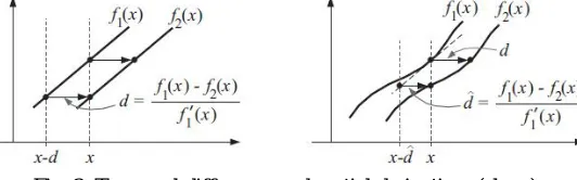
Fig. 2 Temporal difference and spatial derivatives (slope)

In the figure 1, the gradient constraint relates the displacement of the signal to its temporal difference and spatial derivatives (slope). For a displacement of a linear signal (left), the difference in signal values at a point divided by the slope gives the displacement. For nonlinear signals (right), the difference divided by the slope gives an approximation to the displacement.

To derive an estimator for 2D velocity u, we first consider the 1D case. Let f1(x) and f2(x) be 1D signals (images) at two time instants. As depicted in Fig. 1, suppose further that f2(x) is a translated version of f1(x); i.e., let f2(x) = f1(x−d) where d denotes the translation. A Taylor series expansion of f1(x − d) about x is given by

f1(x - d) = f1(x) - d f 1’(x) + O(d2f 1’’’)…………(4.2)

where f’ ≡ (d f(x))/dx. With this expansion we can rewrite the difference between the two signals at location x as f1(x) - f2(x) = d f 1(x) + O(d2f 1’’ )

The 1D case generalizes straightforwardly to 2D. As above, assume that the displaced image is well approximated by a first-order Taylor series:

I(x + u, t + 1) ≈ I(x, t) + u • ∇I(x, t) + It(x, t)……….(4.4)

where ∇I ≡ (Ix, Iy) and It denote spatial and temporal partial derivatives of the image I, and u = 〖(u1,u2)〗^T denotes the 2D velocity. Ignoring higher-order terms in the Taylor series and then substituting the linear approximation into (4.1), we obtain x =(x,y)〗^T and time t, a9nd u = 〖(u1,u2)〗^T is the 2D velocity. Obviously, brightness steadiness once in a while holds precisely. The basic presumption is that surface brilliance stays settled starting with one frame then onto the next. One can manufacture scenes for which this holds; e.g., the scene may be compelled to contain just Lambertian surfaces (no specularities), with an inaccessible point source (so changing the separation to the light source has no impact), no object turns, and no optional brightening (shadows or between surface reflection).

∇I(x, t) · u + It(x, t)=0………(4.5)

Equation (4.5) relates the velocity to the space-time image derivatives at one image location, and is often called the gradient constraint equation. If one has access to only two frames, or cannot estimate It, it is straightforward to derive a closely related gradient constraint, in which It(x, t) in (1.5) is replaced by δI(x, t) ≡ I(x, t + 1) − I(x, t) [6].

IV. PROBLEMDEFINITION

Human action recognition is a vital as well as quite challenging problem in computer vision and machine learning[1]. When a training data set is available, the videos can be provided with labels, but these won’t be as much informative. As these labels are for humans and such labels do not provide any semantic meaning.

The problem to which solution is sleeked is that when a unlabelled video is provided, it can be a difficult task for the computer/machine to determine the class of the video, to which it belongs[5]. A common method incorporated is that, feature vectors or interest points from the videos in the training data set, are extracted from videos belonging to same sort of class, to form various groups. Now for the testing video, feature vectors are extracted and these feature vectors are compared with the feature vectors of the videos in the training dataset[2]. After comparison label of the group which was closest from the training dataset is given to the testing video. SIFT is the prominent strategy for acquiring neighbourhood descriptors

Our objective is to attain human action recognition in a simpler way without extracting interest points, keypoints or feature vectors of the videos in the dataset [11]. Optical flow estimation is used for the same. Rather than going for interest points or keypoints in a frame, whole frame is taken into consideration. Whole frame means each pixel in the image. Frames are selected rather than considering adjacent frames in the video

V. PROPOSEDMETHOD

A database has been made by choosing videos from the UCF Sports dataset. This dataset contains videos of practical activities in various conditions. UCF Sports dataset comprises of different games activities gathered from broadcast television channels. It has videos of total 10 activities. We can add considerably more videos to the database in future if required for analysis[15].

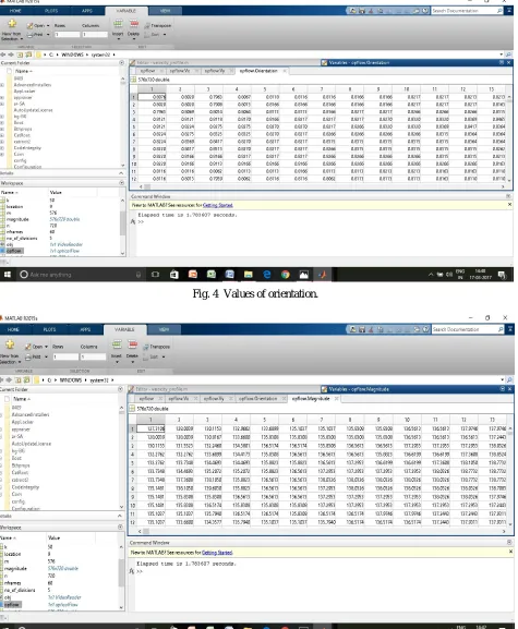
In our method, we are first finding the difference in orientation and magnitude of two frames in the video’s of our database. The orientation and magnitude can be seen in figure 4 and 5 respectively. Initially only two frames are considered. Number of frames into consideration can be increased. The assumption we have made is that, we have not considered the initial few and also final few frames in the video . This is because there might not be as much information in those frames and also factors like camera shutter come into picture.

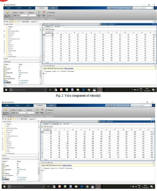
To find the optical flow between frames , optical flow function available in MATLAB is used. This function gives back four parameters, velocity in x direction, velocity in y direction, orientation and magnitude between 90 degrees. In figure 2, the x component of velocity i.e. Vx for all the pixels in the frame is shown. In figure 3, the y component of velocity i.e. Vy for all the pixels in the frame is shown.

Fig. 2 Vx(x component of velocity)

Fig. 3 Vy(y component of velocity)

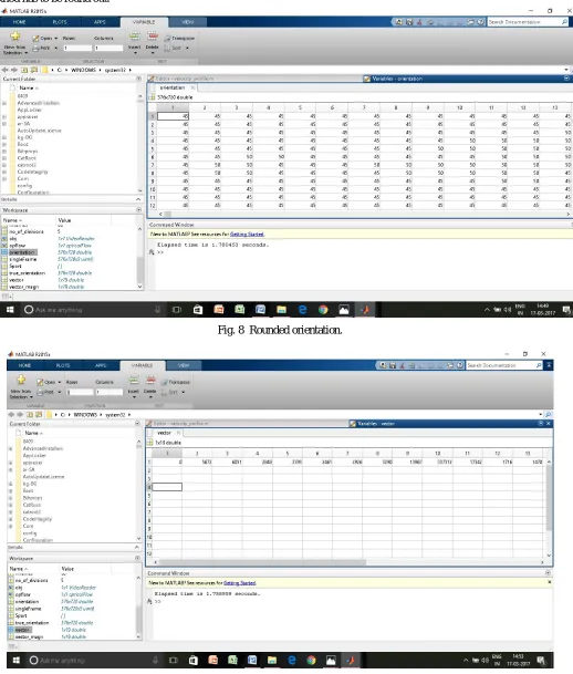
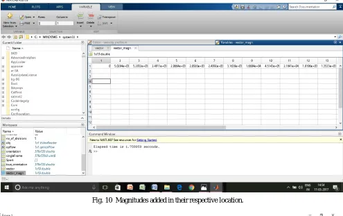
are in degrees. Also these values have to be rounded. These rounded values are stored in a new array as shown in figure 8. Whenever a certain orientation falls in a certain bin, the value of that bin is incremented by 1, as can be seen in figure 9. Magnitude has been scaled down first, see figure 7, as the rate of increase in magnitude fromone frame to other is also vital and will be considered for future analysis. Magnitudes falling in a certain bin are added up together, as shown in figure 10.

Fig. 4 Values of orientation.

Once the difference in orientation and magnitude for all the videos in the database has been calculated, vast informatio regarding the orientation and magnitude will be available. Also a bin size for all the games will be finalized. The efficiency of our proposed method has to be found out.

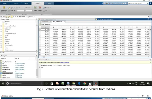
Fig. 6 Values of orientation converted to degrees from radians

Once the difference in orientation and magnitude for all the videos in the database has been calculated, vast information regarding the orientation and magnitude will be available. Also a bin size for all the games will be finalized. The efficiency of our proposed method has to be found out.

Fig. 8 Rounded orientation.

The graph shown in figure 11, is the plot of the difference in orientation and magnitude of all the pixels in the two selected frames. This procedure will be done on all the videos present in our database and that will be used for analysis of finding the action/sports played in the test video.

Fig. 10 Magnitudes added in their respective location.

VI. CONCLUSION

In this paper, optical flow to perform Human Action Recognition is been calculated. In the existing methods, feature vectors, interest points or keypoints are extracted. This step has been skipped in our method, expecting it to reduce the complexity in extracting features, as these extracted features could be scale variant or invariant. But rather entire frame is considered, i.e. all the pixels in the frame. Assumption made is, initial and final frames in the video wont contain major information because of factors like camera shutter, hence those frames are not considered in calculating the optical flow. The difference in orientation and magnitude are computed between the selected frames. Later these values of orientation and magnitude are placed into bins. Competitive result as compared to other methods is expected.

REFERENCES

[1] J. T. Zhang, A. C. Tsoi and S. L. Lo, "Scale Invariant Feature Transform Flow trajectory approach with applications to human action re999cognition," 2014 International Joint Conference on Neural Networks (IJCNN), Beijing, 2014, pp. 1197-1204.

[2] J. K. Aggarwal and Q. Cai, Human motion analysis: A review, Computer Vision and Image Understanding, vol. 73(3), pp. 428-440, 1999. .

[3] Haiam A. Abdul-Azim, Elsayed E. Hemayed, Human action recognition using trajectory-based representation, Egyptian Informatics Journal, Volume 16, Issue 2, July 2015, Pages 187-198, ISSN 1110-8665.

[4] Osama Masoud, Nikos Papanikolopoulos, A method for human action recognition, Image and Vision Computing, Volume 21, Issue 8, 1 August 2003, Pages 729-743, ISSN 0262-8856.

[5] http://cs.stanford.edu/~amirz/index_files/Springer2015_action_chapter.pdf as assessed on 07/08/2017.

[6] D. Sun, S. Roth and M. J. Black, Secrets of Optical Flow Estimation and Their Principles, IEEE Conference on Computer Vision and Pattern Recognition(CVPR), 2010.

[7] K. Schindler and L. van Gool, "Action snippets: How many frames does human action recognition require?," 2008 IEEE Conference on Computer Vision and Pattern Recognition, Anchorage, AK, 2008, pp. 1-8.

[8] C. Thurau and V. Hlavac, "Pose primitive based human action recognition in videos or still images," 2008 IEEE Conference on Computer Vision and Pattern Recognition, Anchorage, AK, 2008, pp. 1-8.

[9] S. Ji, W. Xu, M. Yang and K. Yu, "3D Convolutional Neural Networks for Human Action Recognition," in IEEE Transactions on Pattern Analysis and Machine Intelligence, vol. 35, no. 1, pp. 221-231, Jan. 2013

[10] Y. Zhao, Y. Zhai, E. Dubois and S. Wang, "Image matching algorithm based on SIFT using color and exposure information," in Journal of Systems Engineering and Electronics, vol. 27, no. 3, pp. 691-699, June 22 2016

[11] J. J. Seo, J. Son, H. I. Kim, W. De Neve and Y. M. Ro, "Efficient and effective human action recognition in video through motion boundary description with a compact set of trajectories," 2015 11th IEEE International Conference and Workshops on Automatic Face and Gesture Recognition (FG), Ljubljana, 2015, pp. 1-6

[12] http://www.cs.toronto.edu/~fleet/research/Papers/flowChapter05.pdf as assessed on 07/08/2017.

[13] Berthold K.P. Horn, Brian G. Schunck, Determining optical flow, Artificial Intelligence, Volume 17, Issue 1, 1981, Pages 185-203, ISSN 0004-3702,

http://dx.doi.org/10.1016/0004-3702(81)90024-2.

[14] http://lmi.bwh.harvard.edu/papers/pdfs/gunnar/farnebackSCIA03.pdf as assessed on 07/08/2017 [15] http:/crcv.ucf.edu/data/UCF_Sports_Action.php as assessed on 07/08/2017.