Improving Statistical Learning within
Functional Genomic Experiments by
means of Feature Selection
Osama Mahmoud
A thesis submitted for the degree of
Doctor of Philosophy (Ph.D.)
Department of Mathematical Sciences
University of Essex
Dedicated to
My parents, affectionate wife and adorable children (Seif, Malak and Salma)
Acknowledgements
It is a pleasure to thank those who helped me to make this thesis possible. Foremost, I
would like to express my sincere gratitude to my supervisors Prof. Berthold Lausen and Dr.
Andrew Harrison (Harry) for their continuous support during my PhD study and research.
I am grateful for their patience, motivation, enthusiasm, and immense knowledge. Their
guidance helped me throughout the research and thesis writing period. I could not imagine
having better supervisors for my PhD study. Thanks Berthold and Harry for showing your
trust in me!
There are many other people who supported me throughout my PhD. I owe my deepest
gratitude to Dr. Aris Perperoglou for his help and suggestions whenever needed. Thanks
Aris for your efforts to explain things clearly and simply. My sincere thanks also goes to Dr. Benjamin Hofner, Dr. Werner Adler and Dr. Andreas Mayr, biostatisticians at Institut für
Medizininformatik, Biometrie und Epidemiologie, University of Erlangen, Germany, for
everything I have learnt from them. Thanks to my Supervisory Board members Dr. John
Ford and Dr. Haslifah Hashim who gave me valuable feedbacks and suggestions. Thanks
for all the staffat the Department of Mathematical Sciences, University of Essex for their kindness and support.
I also thank Camilla Thomsen and Claire Watts (previous and current Departmental
Acknowledgements iv
Administrator respectively), Anne Owen (Computer Support Officer), Shauna McNally (Graduate Administrator) and Vicki Forster (General Administrator) for their help in
ad-ministrative issues.
I am grateful to the Helwan University, the Egyptian Ministry of Higher Education and
the Egyptian Cultural and Education Bureau (ECEB) in London for sponsoring my PhD
research. I equally thank Prof. Essam Abouelkassem, Prof. Afaf El-Dash, Prof. Ibrahim
Hassan, Dr. Nadia Khalifa, Dr. Sayed El-Shair and Dr. Ahmed Abdelhadi whose support
will be remembered always.
I wish to thank my entire family and my family-in-law for their love and support. I
particularly thank my parents, Fathy Mahmoud and Nema Saad, and my younger sister
and brother, Shaimaa Mahmoud and Abdelhaleem Mahmoud, who have been a great
source of motivation. Thanks also goes to friends for their prayers and emotional support.
Lastly but importantly, I thank my wife, Doaa Saeed Ibrahim, for her love and care.
Thanks for being with me in hard times and for your emotional support whilst you were
also busy in looking after our children. For my children, Seif, Malak and Salma Mahmoud,
Abstract
A Statistical learning approach concerns with understanding and modelling complex
datasets. Based on a given training data, its main aim is to build a model that maps
the relationship between a set of input features and a considered response in a predictive
way. Classification is the foremost task of such a learning process. It has applications
en-compassing many important fields in modern biology, including microarray data as well
as other functional genomic experiments.
Microarray technology allow measuring tens of thousands of genes (features)
simulta-neously. However, the expressions of these genes are usually observed in a small number,
tens to few hundreds, of tissue samples (observations). This common characteristic of high
dimensionality has a great impact on the learning processes, since most of genes are noisy,
redundant or non-relevant to the considered learning task.
Both the prediction accuracy and interpretability of a constructed model are believed
to be enhanced by performing the learning process based only on selected informative
features. Motivated by this notion, a novel statistical method, named Proportional
Over-lapping Scores (POS), is proposed for selecting features based on overOver-lapping analysis
of gene expression data across different classes of a considered classification task. This method results in a measure, calledPOSscore, of a feature’s relevance to the learning task.
Abstract vi
POS is further extended to minimize the redundancy among the selected features.
The proposed approaches are validated on several publicly available gene expression
datasets using widely used classifiers to observe effects on their prediction accuracy. Selec-tion stability is also examined to address the captured biological knowledge in the obtained
results. The experimental results of classification error rates computed using the Random
Forest,kNearest Neighbor and Support Vector Machine classifiers show that the proposals
Declaration
The work submitted in this thesis is the result of my own investigation, except where
otherwise stated. It has not already been accepted for any degree, and is also not being
concurrently submitted for any other degree.
Copyright c 2015 by Osama Mahmoud.
“The copyright of this thesis rests with the author. No quotations from it should be
published without the author’s prior written consent.”
Abbreviations
Abbreviations Details
Bagging Bootstrap Aggregation
CART Classification and Regression Trees RF Random Forest
kNN k Nearest Neighbour SVM Support Vector Machine
KKT Karush-Kuhn-Tucker conditions C.V. Cross Validation
LASSO Least Absolute Shrinkage and Selection Operator POS Proportional Overlapping Scores method
Wil-RS Wilcoxon Rank Sum test method
ISIS Iteratively Sure Independent Screen method
mRMR minimum Redundancy Maximum Relevance method MP MaskedPainter method
POS Proportional Overlapping Score measure
RDC Relative Dominant Class measure
|.| Size of a set{.}
hIi length of the intervalI
Contents
Acknowledgements iii Abstract v Declaration vii Abbreviations viii Contents ixList of Figures xiv
List of Tables xvi
List of Algorithms xviii
1 Introduction 1
1.1 Introduction . . . 1
1.2 Thesis Organization . . . 4
1.3 Published Work . . . 6
2 Background for Statistical Learning 7
Contents x
2.1 Supervised vs. Unsupervised Learning . . . 7
2.2 Classification and Regression Trees (CART) . . . 8
2.2.1 Best Split of Nodes . . . 10
2.3 Supervised Ensemble Learning . . . 13
2.3.1 Ensemble Learning Algorithms . . . 13
2.3.2 Ensemble Combining Methods . . . 18
2.3.3 Ensemble Diversity . . . 19
2.4 Random Forest . . . 20
2.5 kNearest Neighbour . . . 24
2.6 Support Vector Machine . . . 27
2.7 Classifier Performance Evaluation via Cross Validation . . . 32
2.8 Summary . . . 33
3 Feature Selection 35 3.1 Introduction . . . 35
3.2 Gene Selection . . . 36
3.3 Methods of Gene Selection . . . 38
3.3.1 Wrapper Methods . . . 38
3.3.2 Embedded Methods . . . 39
3.3.3 Filter Methods . . . 39
3.4 Gene Expressions Overlap . . . 41
3.5 Summary . . . 43
Contents xi
4.1 Introduction . . . 45
4.2 Definition of Core Intervals . . . 48
4.3 Gene Masks . . . 50
4.4 The ProposedPOSMeasure . . . 51
4.5 Identifying the Minimum Subset of Genes . . . 53
4.6 Summary . . . 56
5 Proportional Overlapping Score Method for Gene Selection 57 5.1 The Method . . . 59
5.1.1 Relative Dominant Class Assignments . . . 59
5.1.2 Final Gene Selection . . . 60
5.1.3 Illustrative Example . . . 61
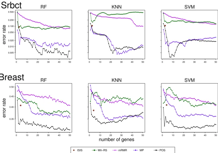
5.2 Results . . . 64
5.2.1 POS Method Quality Performance . . . 71
5.2.2 Minimum Misclassification Error . . . 74
5.2.3 Stability Evaluation . . . 74
5.3 Summary . . . 81
6 Minimizing Redundancy among Selected Genes 83 6.1 Recursive Minimum Sets for Minimizing Selection Redundancy (POSr) . . . 84
6.1.1 The Method . . . 84
6.1.2 Illustrative Example . . . 89
6.2 Results . . . 90
Contents xii
7 Conclusions and Future Plans 99
7.1 Conclusions . . . 99
7.2 Future Plans . . . 103
Appendices 105 A Availability of Supporting Data 105 A.1 The Lung Dataset . . . 105
A.2 The Leukaemia Dataset . . . 105
A.3 The Srbct Dataset . . . 106
A.4 The Prostate Dataset . . . 106
A.5 The Carcinoma Dataset . . . 107
A.6 The Colon Dataset . . . 107
A.7 The All Dataset . . . 107
A.8 The Breast Dataset . . . 107
A.9 The GSE24514 Dataset . . . 108
A.10 The GSE4045 Dataset . . . 108
A.11 The GSE14333 Dataset . . . 108
A.12 The GSE27854 Dataset . . . 109
B Classification Error Rates 110 B.1 Classification Error Rates Obtained by Random Forest . . . 110
B.2 Classification Error Rates Obtained bykNearest Neighbor . . . 116
Contents xiii
List of Figures
2.1 An example for the basic CART structure . . . 9
2.2 Impurity measures for binary classification problems . . . 12
2.3 k-nearest neighbour framework . . . 25
2.4 Support vector classifier in a 2-dimensional feature space . . . 28
4.1 An example for two different genes with different overlapping pattern. . . . 47
4.2 Core expression intervals with gene mask . . . 51
4.3 Illustration for overlapping intervals with different proportions . . . 53
5.1 Building blocks of POS method . . . 61
5.2 An illustrative example of the POS method . . . 63
5.3 Averages of classification error rates for ‘Srbct’ and ‘Breast’ datasets . . . 70
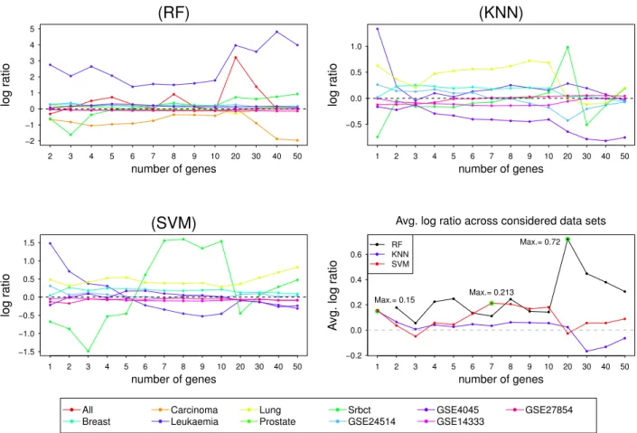
5.4 Log ratio between the error rates of the best compared method and the POS 72 5.5 Stability scores for ‘GSE27854’ dataset . . . 77
5.6 Stability scores for ‘GSE24514’ dataset . . . 78
5.7 Stability-accuracy plot for ‘Lung’ dataset . . . 79
5.8 Stability-accuracy plot for ‘GSE27854’ dataset . . . 80
6.1 An illustrative example of the POSr approach . . . 89
List of Figures xv
6.2 Averages of classification error rates for ‘Srbct’ and ‘Breast’ datasets with
POSr method . . . 91
6.3 Stability scores for ‘GSE24514’ dataset . . . 96
List of Tables
5.1 Description of used gene expression datasets . . . 65
5.2 Average classification error rates yielded by Random Forest, k Nearest
Neighbors and Support Vector Machine classifiers on ‘Leukaemia’ dataset . 68
5.3 Average classification error rates yielded by Random Forest, k Nearest
Neighbors and Support Vector Machine classifiers on ‘GSE24514’ dataset . . 69
5.4 The minimum error rates yielded by Random Forest classifier with feature
selection methods along-with the classification error without selection . . . 75
5.5 The minimum error rates yielded by k Nearest Neighbor classifier with
feature selection methods along-with the classification error without selection 75
5.6 The minimum error rates yielded by Support Vector Machine classifier with
feature selection methods along-with the classification error without selection 76
5.7 Stability scores of the feature selection techniques for the ‘Srbct’ dataset . . 77
6.1 Average classification error rates yielded by Random Forest, k Nearest
Neighbors and Support Vector Machine classifiers on ‘Leukaemia’ dataset . 92
6.2 Average classification error rates yielded by Random Forest, k Nearest
Neighbors and Support Vector Machine classifiers on ‘Leukaemia’ dataset . 93
List of Tables xvii
6.3 Comparison between the minimum error rates yielded by the feature
List of Algorithms
2.1 Bootstrap Aggregation (Bagging) for Classification Trees . . . 15
2.2 Boosting . . . 17
2.3 Random Forest for Classification . . . 21
4.1 Greedy Search - Minimum set of genes . . . 54
5.1 POS Method For Gene Selection . . . 62
6.1 POSr Method: Recursive Minimum Subsets . . . 86
Chapter 1
Introduction
1.1
Introduction
Statistical Learning refers to a set of approaches for constructing a predictive model based
on a given dataset. It encompasses many methods including Classification Trees (Breiman
1984), Random Forest (Breiman 2001), Boosting (Freund & Schapire 1997), k Nearest
Neigh-bour (Cover & Hart 1967) and Support Vector Machines (Cortes & Vapnik 1995). The main
goal of statistical learning is to train a given set of data, training data, to model an effective prediction rule that can be then used to predict unseen/new data.
The recent revolution in functional genomic technologies leads to generate vast amount
of data. Microarray, as well as other high-throughput functional genomic technologies,
provide effective tools for studying thousands of genes simultaneously. The challenge of understanding these data has led to the development of new tools in statistical learning.
Classification is the foremost task of statistical learning within the biological domain
(Fried-man et al. 2001). For a particular classification task, microarray data are inherently noisy
1.1. Introduction 2
since most genes are irrelevant and uninformative to the given classes (phenotypes).
Both the prediction accuracy and interpretability of a constructed classifier could be
enhanced by performing the learning process based only on selected informative features.
One of the main aims of gene expression analysis is to identify genes that are expressed
differentially between various classes. The problem of identification of these discriminative genes for their use in classification has been investigated in many studies (Chen et al. 2014,
Apiletti et al. 2012, Peng et al. 2005).
A major challenge is the problem of dimensionality; tens of thousands of genes’
expres-sions are observed in a small number, tens to few hundreds, of observations. Given an
input of gene expression data along-with observations’ target classes, the problem of gene
selection is to find among the entire dimensional space a subspace of genes that best
char-acterizes the response target variable. Since the total number of subspaces with dimension
not higher than r is Pr
i=1
P i
, where P is the total number of genes, it is hard to search the
subspaces exhaustively.
Alternatively, various search schemes are proposed e.g., best individual genes (Su et al.
2003), Max-Relevance and Min-Redundancy based approaches (Peng et al. 2005), Iteratively
Sure Independent Screening (Fan et al. 2009) and MaskedPainter approach (Apiletti et al.
2012). Identification of discriminative genes can be based on different criteria including: p-values of statistical tests e.g. t-test or Wilcoxon rank sum test (Lausen et al. 2004, Altman
et al. 1994); ranking genes using statistical impurity measures e.g. information gain, gini
index and max minority (Su et al. 2003).
Here, the overlap between gene expression measures for different classes is utilized. The thesis provides a strategy that uses the information given by observations’ classes as
1.1. Introduction 3
well as expression data for detection of the differentially expressed genes between target classes. The possibility of improving a classifier performance and prediction accuracy by
identifying discriminative genes that are relevant to the considered classification task is
investigated.
The thesis proposes a procedure that analyses the overlap between gene expression of
different classes, to identify the minimum set of genes which yield the best classification accuracy on a training set whilst avoiding the effects of outliers. Based on this procedure, a novel statistical method, named as Proportional Overlapping Scores (POS), is proposed for
selecting discriminative features for a considered classification task. This method results
in a measure, calledPOSscore, of a feature’s relevance to the classification problem.
Several widely used classifier models: Random Forest; k Nearest neighbour; Support
Vector Machines, are used to evaluate the efficiency of the proposed approach in improv-ing the learnimprov-ing process. POS method is validated on 12 publicly available gene
expres-sion datasets by comparison with five well-known gene selection techniques: Wilcoxon
Rank Sum (Wil-RS); Minimum Redundancy Maximum Relevance (mRMR); MaskedPainter
(MP); Iteratively Sure Independent Screening (ISIS). The experimental results of
classifi-cation error rates computed using the considered classifiers show that POS achieves a
better performance. The proposed approach with the conducted experiments have been
published in Mahmoud et al. (2014a).
The POS method is further extended to minimize the redundancy among the selected
features. A recursive strategy is proposed to assign a set of complementary informative
genes. The scheme exploits gene masks defined by POS to identify more integrated genes
1.2. Thesis Organization 4
published in Mahmoud et al. (2015)
The approaches proposed in this thesis are implemented in an R-package, called
‘propOverlap’, publicly available on CRAN (Mahmoud et al. 2014b).
1.2
Thesis Organization
Chapter 2 provides a background for statistical learning. It illustrates the difference be-tween supervised and unsupervised learning and also discusses the basics of classification
and regression trees (CART) and ensemble learning schemes. Detailed explanation of
sev-eral classification models such as Random Forest, k Nearest Neighbour and Support Vector
Machine are also provided. Finally, some methods and metrics for evaluating a classifier
performance are described.
Chapter 3 illustrates different approaches for feature selection. Different categories of feature selection methods are described. The chapter also introduces the general criterion
of gene expressions overlap for identifying discriminative genes.
Chapter 4 proposes a procedure for identifying the minimum subset of genes that
pro-vide the best classification accuracy on a set of given training data. The procedure propro-vides
a definition of gene mask that measure the classification power of each gene in a
consid-ered binary classification problem. This chapter also presents a novel score, POS, for
measuring the overlapping degree between expressions of different classes. An algorithm for detecting the minimum set of genes that correctly classify the maximum number of
1.2. Thesis Organization 5
been published (Mahmoud et al. 2014a).
Chapter 5 proposes a novel method, named ‘POS’, for gene selection based on the defined
POSscore along-with the minimum subset of genes. The chapter also shows the results of
misclassification error rates obtained by POS using Random Forest, k Nearest Neighbour
and Support Vector Machine classifiers. The results from POS are compared with the ones
yielded by widely used gene selection methods such as Wilcoxon Rank Sum (Wil-RS),
Min-imum Redundancy MaxMin-imum Relevance (mRMR), MaskedPainter (MP), Iteratively Sure
Independent Screening (ISIS). Scores of stability selections are provided for the proposed
approach and the compared methods. This work has been published in Mahmoud et al.
(2014a).
Chapter 6 proposes an extended version of POS method, named ‘POSr’, for minimizing
the selection redundancy using a recursive strategy to assign a set of complementary
discriminative genes. This chapter shows the misclassification error rates as well as stability
scores for the proposed approach. The obtained results are compared with POS and other
gene selection methods. The research within this chapter has been published in Mahmoud
et al. (2015).
Chapter 7 summarises the conclusions of the thesis and suggests future directions in
1.3. Published Work 6
1.3
Published Work
Peer-reviewed Papers:
1. Mahmoud, O., Harrison, A., Perperoglou, A., Gul, A., Khan, Z., Metodiev, M. &
Lausen, B. (2014a): A feature selection method for classification within functional
genomics experiments based on the proportional overlapping score, BMC
Bioinfor-matics 15(1).
2. Mahmoud, O., Harrison, A., Gul, A., Khan, Z., Metodiev, M. & Lausen, B. (2015):
Minimizing redundancy among genes selected based on the overlapping analysis,
in Proceedings of the European Conference on Data Analysis, Bremen, Germany [In
Press].
Published R Packages:
1. Mahmoud, O., Harrison, A., Perperoglou, A., Gul, A., Khan, Z. & Lausen, B. (2014b):
propOverlap: Feature (gene) selection based on the Proportional Overlapping Scores.
Chapter 2
Background for Statistical Learning
Statistical learning techniques are described as eithersupervised,semi-supervisedor
unsuper-vised. The distinction results from how the learning process identifies its training data.
2.1
Supervised vs. Unsupervised Learning
In supervised learning, training data are usually presented as (X,Y) such thatX ∈ ℜN×Pis
a feature matrix in whichNobservations are reported each with Pfeatures (dimensions),
whilst Y ∈ ℜN is a vector of output labels (supervisors). Classification techniques (e.g.,
Classification and Regression Trees, Random Forest, k Nearest Neighbour and Support
Vector Machine, presented in Sections 2.2, 2.4, 2.5 and 2.6 respectively) provide important
representative examples of supervised learning.
Unsupervised learning defines the training data to contain only the feature matrix
X (i.e., N observations are presented each with P features without supervised output
labelsY). Clustering techniques (e.g.,kmeans and hierarchical clustering) are the classical
2.2. Classification and Regression Trees (CART) 8
representative examples for unsupervised learning.
Semi-supervised learning falls between unsupervised learning and supervised learning.
It refers to a set of tasks and techniques that treat data with supervised output labels for
part of it.
2.2
Classification and Regression Trees (CART)
Classification and Regression Trees (CART) have been around since Breiman et al. (1984)
proposed a procedure for building trees to predict categorical and continuous response
variables for classification and regression problems respectively. Many refinements of
CART approach have been developed for enhancing its uses in various fields (e.g., Chipman
et al. 1998, Loh 2002, Su et al. 2004). CART are considered a base classifier for most of the
ensemble learning methods which are discussed in Section 2.3. They are used in many
fields including statistics, applied mathematics and computer science, etc. Moreover, they
are usually linked to machine and statistical learning, and data mining.
The CART approach uses the training data to construct a binary decision tree which is
then used for predicting the class labels of new data (in case of classification problems) or
the real-values of the response (in case of regression). This is accomplished by recursively
splitting the feature space into two disjoint regions (e.g., two outcomes in the case of a
binary feature (for more details, see Section 2.2.1)).
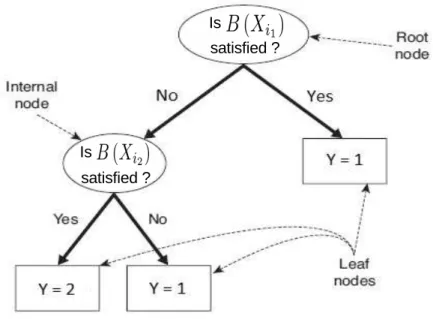
For classification problems, a set of training data (X,Y) are given. Figure 2.1 illustrates
the structure of CART whereXil,l= 1,2 are two features (predictors) andB Xil
is a given
2.2. Classification and Regression Trees (CART) 9
Figure 2.1: An example for the basic CART structure
full training data while each of the internal and leaf nodes contains a subset of the data
associated with its parent node. The whole structure of a classification tree is accomplished
via a recursive binary splitting procedure applied for each node. This procedure aims to
separate the training data into reasonably purer subsets in terms of their classes distribution.
A stop condition is employed to terminate the splitting process.
Generally, an exponential number of distinct classification trees can be built from a given
set of features. While some of them are more accurate than others, finding the optimal
tree is computationally infeasible for high dimensional datasets due to the exponential
size of the entire search space (Tan et al. 2007). Nevertheless, many algorithms have been
developed for building a reasonably accurate CART in a reasonable amount of time. These
algorithms usually grow a tree by making a series of locally optimum decisions about
2.2. Classification and Regression Trees (CART) 10
2.2.1
Best Split of Nodes
The CART algorithm provides a tool for determining a test condition B(Xi), associated
with featureXi, that should be selected among different feature types in order to get the
best split for a given node.
For binary features, the test conditionB(Xi) generates two potential outcomes by which
a two-way split is formed.
Nominal features having many values produce a test condition which can be expressed
either into multi-way split or a two-way split. For the former splitting way, each outcome
corresponds to one of the feature distinct values. For the latter way, splitting is
accom-plished by grouping the feature values into two non-empty disjointed subsets. Some
algorithms, such as CART, produce only two-way (binary) splits by considering all the
2m−1−1 ways of creating a binary partition ofmfeature values.
Similarly, ordinal features can produce multi-way or binary split providing that the
grouping process, if any, does not violate the order of the feature values.
Finally, for continuous features, the test condition B(Xi) can be expressed as a
compar-ison test with binary outcomes (Xi ≤ αVs.Xi > α). Otherwise, it could be presented as a
range query with outcomes of the formαi <Xi ≤αi+1, i=1, . . . ,m. One possible approach is discretizing the continuous values into ordinal intervals. Afterwards, each new ordinal
value will be assigned to one outcome of a multi-way split. Also, adjacent intervals can be
grouped into binary outcomes as long as the order is preserved (Tan et al. 2007).
It is essential to define an objective measure for evaluating the goodness of each test
condition, and then identifying the best test condition. This goodness of a test condition is
2.2. Classification and Regression Trees (CART) 11
and after splitting using that condition. On this basis, the best is the one which leads to
lowest impurity of observations class distribution before and after splitting.
Measures for detecting the best split
Selection of the best split is based on the degree of impurity. An objective measure can be
defined for evaluating the goodness of the split by comparing the degree of impurity of
the parent with those of child nodes. The most widely used impurity measures (Friedman
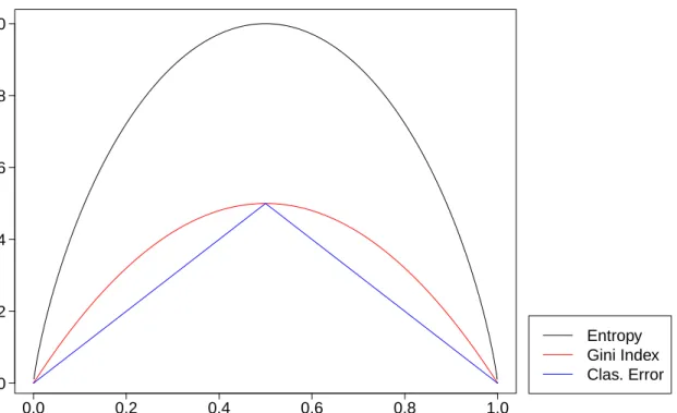
et al. 2001),Gini Index,EntropyandClassification Error, are shown respectively in (2.1)-(2.3).
Gini Index(t)=1− C X c=1 θ2ct, (2.1) Entropy(t)=−X c∈St θctlog2θct, St ={c|θct,0, c=1, . . . ,C}, (2.2)
Classi f ication Error(t)=1−max
c θct, (2.3)
whereθctdenotes the proportion of observations belonging to classcamong all observations
at a given node t, and Cis the number of classes. For Entropy measure, the summation
is only over the non-empty classes, (i.e., classes for whichθct , 0). Impurity degree for a
nodet can be computed using these measures. Smaller values represent more skewness
for the class distribution of given observations, thus more benefits for splitting purposes.
Figure 2.2 shows the values of these measures for binary classification situations (when
C =2). In this case, θctrepresented by the x-axis in Figure 2.2, can refer to any of the two classes sinceθ1t =1−θ2t.
Now, the goodness of a test condition at a node t can be evaluated by comparing
2.2. Classification and Regression Trees (CART) 12 0.0 0.2 0.4 0.6 0.8 1.0 0.0 0.2 0.4 0.6 0.8 1.0
θct
Impur
ity
Entropy Gini Index Clas. ErrorFigure 2.2:Impurity measures for binary classification problems
splitting, with impurity degrees of the resulted child nodes, after splitting. The best
condition is the one which leads to the largest difference between impurity degrees of before and after splitting. The criterion used for determining goodness of a node split is
called “gain” and denoted by△such that (Friedman et al. 2001):
△t =I(t)− m X β=1 ntβ nt .Itβ (2.4) where Itβ
is the computed impurity of the child node tβ, whereas ntβ refers to the
number of observations associated with it, while m represents the number of children
nodes (feature outcomes). Algorithms often choose a test condition that maximizes △or equivalently minimizes the weighted average impurity measures of the child nodes asI(t)
2.3. Supervised Ensemble Learning 13
2.3
Supervised Ensemble Learning
Ensemble learning was originally presented for supervised learning, specifically
classifica-tion problems, in 1965 (Nilsson 1965). The basic concept of supervised ensemble learning
is to train multiple base classifiers which are basically designed for the same task, then
combine their predictions into a single ensemble classifier. This classifier should perform
better than any member of base classifiers; otherwise, ensemble process doesn’t make
sense. In general, diverse weak base classifiers together can produce a strong ensemble
classifier if they are given an opportunity to operate within the same procedures. This
technique allows better performance, in terms of both generality and accuracy, than could
be achieved via any single base classifier. For classification tasks, many researchers have
demonstrated the outstanding performance of ensemble learning (Ho et al. 1994, Cho &
Kim 1995, Breiman 1996, Oza & Tumer 2001, Dietterichl 2002, Tumer & Oza 2003).
An ensemble procedure should address some fundamental issues such as: how to train
each of the single bases (learning algorithm); how to combine their predictions (combining
method); how to measure the diversity as a necessary but not sufficient condition of ensemble learning efficiency (diversity). These fundamental arguments are discussed sequentially in Sections 2.3.1 - 2.3.3.
2.3.1
Ensemble Learning Algorithms
Multiple base classifiers can be trained either individually in a parallel system or
co-ordinately in a sequential system. Two of the most common ensemble algorithms, Bagging
2.3. Supervised Ensemble Learning 14
powerful algorithms give explicit examples for these different strategies of ensemble meth-ods.
Bagging algorithms
It is one of the simplest and well-known ensemble algorithms. Originally, Bootstrap
aggregation (bagging) was introduced in Breiman (1996) for supervised ensemble learning.
However afterwords, the idea has been extended for unsupervised learning. Fischer &
Buhmann (2003) developed uses of the bagging algorithm for some clustering tasks. In
addition, Dudoit & Fridlyand (2003) demonstrated the efficiency of using bagging for improving the accuracy of clustering.
The main idea is based on building successive base learners. Each of them is
con-structed using a bootstrap sample of the considered dataset. Then, a majority vote is taken
for prediction. For instance, bagging of the classification trees is conducted by building
successive trees using bootstrap samples of the training dataset. Then, the majority vote
of predicted classes is taken for the output prediction of bagging. The ensemble learner is
then able to reduce the variance of the estimated prediction function (Friedman et al. 2001).
A summary of the bagging procedure for classification trees is shown in Algorithm 2.1.
Boosting algorithms
Like bagging, the boosting approach was firstly proposed for a supervised ensemble and
was originally designed for classification problems. Freund & Schapire (1997) introduced
an algorithm named Adaboost which inspired Boosting algorithms for improving
2.3. Supervised Ensemble Learning 15 Algorithm 2.1Bootstrap Aggregation (Bagging) for Classification Trees
Inputs: Set of training data (X, Y).
Output: Ensemble of classification trees{Tb}B1.
1: forb =1to Bdo
2: draw a bootstrap samplesbof sizeNfrom the training dataset.
3: grow a classification treeTbbased on the bootstrapped samplesb.
4: end for
5: return Ensemble of trees,{Tb}B1.
To make a prediction at a new observation xnew:
6: Let ˆfb(xnew) be the class prediction of thebth classification tree.
7: return yˆnew = fˆbagB (xnew)=majority vote
n
ˆ fb(xnew)
oB
1.
2004, Frossyniotis et al. 2004, Saffari & Bischof 2007, Liu et al. 2007) have extended it into unsupervised learning.
The main idea of boosting technique is that a powerful ensemble classifier can be
produced by integrating the outputs of various weak classifiers. From this perspective,
boosting bears a resemblance to bagging. However, we shall illustrate that the similarity
is at best superficial and that boosting is fundamentally different.
The basic idea is that each training individual observation is associated with an adapted
weight based on how the observation was classified in the previous iteration, initial weights
are usually set in a balanced setting at the first iteration. Observations with higher weight
values (more misclassified) are then more likely to be selecting for training data of the
next iteration, paying more attention to observations that are difficult to classify. By sequentially constructing a linear combination of base classifiers which are fitted at each
iteration, boosting can concentrate more on ‘difficult’ individual observations and hence provide an effective ensemble classifier for the considered classification problem.
To illustrate boosting, consider a C-classes classification problem, with the response
2.3. Supervised Ensemble Learning 16
ˆ
y∈ {1, . . . , C}. Then, the misclassification error rate of the classifier fb(X) can be shown as:
errb = 1 N N X j=1 Iyj , yˆj , (2.5) where Iyj , yˆj = 1 i f yj , yˆj 0 Otherwise ,
such that N represents the number of observations in the training dataset, yj and ˆyj are
the observed and the predicted class respectively of the observation j, i = 1, . . . , N. A weak classifier is the one whose error rate is slightly better than the random guessing.
The purpose of boosting is to sequentially fit a base classifier to adaptively versions of the
training dataset, then producing a sequence of classifiers fb(X), b= 1, . . . , Bwhich are
used for classification prediction (Hastie et al. 2009). Consequently, ensemble of these base
classifiers produces a final classifier f(X) whose prediction is a weighted majority vote of
the base classifiers prediction. Thus, prediction of f (X) for the inputxj, the features value
of the jth observation, can be expressed as:
ˆ fboostB xj = argmax c B X b=1 τb·Ifˆb xj = c , c =1, . . . , C. (2.6) where, Ifˆb xj = c=
1 i f jth observation is assigned to class c by classi f ier fb(X)
0 Otherwise
. (2.7)
2.3. Supervised Ensemble Learning 17 Algorithm 2.2Boosting
Inputs: Set of training data (X, Y).
Output: Ensemble classifier fboostB (X).
1: Initialize weights of the observations such thatwj =
1
N, j=1, . . . , N.
2: forb =1to Bdo
3: fit a classifier fb(X) to the training data sampled using the weightswj.
4: errb = N P j=1 wjI(yj,fˆb(xj)) N P j=1 wj
5: based onerrb, calculateτbby which the contribution of the classifier fb(X) is weighted.
6: Update wj based on the current status (misclassified or not) of the jth observation, j=1 . . . , N.
7: end for
8: return the final classifier, fB
boost(X), by aggregating the base classifiers fb(X) associated
with their weightsτb,b =1, . . . , B.
To make a prediction at a new observationxnew:
9: return yˆnew = fˆboostB (xnew)= argmax c B P b=1 τb·Ifˆb(xnew) = c ! , c=1, . . . , C.
the contribution of each base classifier fb(X) and their effect is to give higher impact to the
more accurate classifiers in the sequence. Algorithm 2.2 shows the general procedure of
the boosting technique.
Different boosting algorithms modify the general procedure shown in Algorithm 2.2. For instance, AdaBoostM1 algorithm, the most popular boosting algorithm (Freund &
Schapire 1997), definesτbandwj (lines 5 and 6 respectively in Algorithm 2.2) as follows:
τb = log 1−err b errb , wj ←wj·exp h τb· Iyj , fˆb xj i .
Boosting ensemble algorithm is constructed based on sequential iterations with
perti-nent feedback from the previous base classifier. This is different from parallel algorithm strategies applied in Bagging and Random Forest (introduced in Sections 2.3.1 and 2.4
2.3. Supervised Ensemble Learning 18
respectively).
2.3.2
Ensemble Combining Methods
Whenever multiple base classifiers are constructed, the ensemble learning algorithms
should apply a convenient tool to combine their individual outputs into a single form
of ensemble classifier. There are a large number of methods for model combination. Linear
combiner, the product combiner, and majority voting combiner are the most commonly used
in practice and demonstrate good performance for a numerous applications of ensemble
learning (Brown 2009).
Thelinear combineris for models whose response is a real-valued variable. It is used
for some supervised learning tasks such as regression and classification which produce
estimated class probabilities. For the latter case, the linear combiner can be formulated as
an ensemble probability estimate as follows:
p yˆ|x = B X b=1 τb · pb yˆ|x (2.8)
wherepb yˆ|xis the probability estimate of class labelygiven the input dataxusing the bth base classifier. Whileτbis the assigned weight of thebth classifier.
The product combiner is more suitable than linear under the assumption that the
class probability estimates pb yˆ|x, b = 1, . . . ,B are independent. It is the theoretically
optimal combination strategy under that assumption. This combiner can be formulated by
2.3. Supervised Ensemble Learning 19 pb yˆ|x = 1 γ B Y b=1 pb yˆ|x (2.9)
whereγis a constant functioning as a normalization factor to adjustp yˆ|x
into a form
of a valid distribution (Brown 2009).
Both linear and product combiners are employed if and only if the base classifiers
produce real-valued outputs. When the base classifier instead estimates the class labels,
themajority voting combinercan be used. Using this method, the class label with the most
votes among all trained base classifiers is assigned as the ensemble prediction. Therefore,
the ensemble prediction output using majority vote combiner can be formulated as shown
in Boosting, (cf., (2.6)). When the weights of base classifiers are uniformly distributed (i.e.
τb = 1/B, ∀b), a simple majority voting combiner is employed as in Bagging, (cf., line 7 in Algorithm 2.1).
2.3.3
Ensemble Diversity
An ensemble is performed by complementing a weak single classifier with other base
classifiers, which make errors on different observations, to enhance the diversity among the combined classifiers. Diversity of the base classifiers is considered a necessary but not
sufficient condition for the success of the ensemble learning. The bases have to be diverse and accurate in order to produce an optimal ensemble learning output.
Measurements of ensemble diversity could be divided into two distinct groups, pairwise
measures and non-pairwise measures. In the former group, the difference between a pair of base classifiers is considered one at a time, the ensemble diversity measure is then obtained
2.4. Random Forest 20
by averaging overall differences across all pairs (e.g.,Double-fault measure(Giacinto & Roli 2001) and Disagreement measure (Skalak et al. 1996)). On the other hand, non-pairwise
measures consider all the base classifiers together (e.g., Entropy measure(Cunningham &
Carney 2000),Generalized Diversity(Partridge & Krzanowski 1997),Kohavi-Wolpert Variance
(Kohavi et al. 1996) andMeasure of Difficulty(Hansen & Salamon 1990)).
2.4
Random Forest
The Random Forest (RF) approach was developed by Breiman (2001) as an extension of
the Classification and Regression Trees (CART) technique presented in Section 2.2. The
Bagging algorithm, described in Section 2.3.1, is considered the basis of the Random Forest.
Since Bagging constructs each tree using a different bootstrap sample of the dataset, RF has a similar procedure to Bagging with an additional layer of randomness. RF consists
of bagging of decision tree learners with a randomized selection of predictors at each
split. Unlike CART, each node is split using the best among a randomly chosen subset
of predictors. RF achieves a powerful performance compared to many other classifiers
including discriminant analysis, neural networks and support vector machines, and is
robust against over-fitting (Breiman 2001). The algorithm of RF modified from Hastie et al.
(2009) for classification problems is introduced in Algorithm 2.3.
The main idea of Bagging, shown in Section 2.3.1, is to average many noisy models in
order to reduce the variance of the final ensemble model. Trees are ideal candidates for
applying Bagging since they are famed as noisy models, thus they can benefit greatly from
2.4. Random Forest 21 Algorithm 2.3Random Forest for Classification
Inputs: Set of training data (X, Y).
Output: Random Forest classifier fRF(X).
1: forb =1to ntreedo
2: draw a bootstrap sample,sb, of sizeNform the original dataset.
3: construct a random-forest tree Tb to the bootstrapped sample,sb, by recursively
re-peating the following steps for each terminal node, until reaching the stop condition, which might be minimum node sizenmin or the terminal node contains members of
only one class:
3a: selectmtrypredictors at random from thePpredictors.
3b: choose the best split among thosemtrypredictors.
3c: split the node into two child nodes.
4: end for
5: return the ensemble of trees,{Tb}n1tree.
To make a prediction at a new observation xnew:
6: let ˆfb(xnew) be the class prediction of thebth random-forest treeTb.
7: return fˆRF(xnew)=majority vote
n
ˆ fb(xnew)
ontree
1 .
distributed (i.d.), the expectation of their average is the same as the expectation of any
single tree of them. In other words, the bias of bagged trees is equivalent to the bias of
the individual trees. Hence, the only hope of improvement is via variance reduction. This
idea is in contrast to boosting, shown in Section 2.3.1, as the trees are sequentially grown
to repeatedly reduce the bias, and hence they are not i.d. trees (Hastie et al. 2009).
The variance of the average of ntree i.d. variables T1, . . . , Tntree with variance σ2 and positive pairwise correlationρcan be expressed as:
V 1 ntree T1+. . .+Tntree = 1 ntree2 h
ntree · σ2+ntree(ntree−1)ρσ2
i
= 1−ρ ntree ·
σ2 + ρσ2 (2.10)
Hence, as ntree increases, the first term of (2.10) tends to disappear, but the second
2.4. Random Forest 22
affect the benefits of averaging. A higher correlation between results in a higher variance of the ensemble. The idea of RF (Algorithm 2.3) is to improve the performance by reducing
the variance of bagging through decreasing the correlation between the trees, without
increasing the variance of them too much. This idea can be achieved by selecting mtry
predictors randomly among all thePpredictors at each split through tree-growing process.
This leads to the production of more diverse trees (see ensemble diversity in Section
2.3.3). Therefore, Bagging can be thought of as the special case of RF obtained when
mtry = P. Usually, mtry values are chosen as
√
P, which is the default setting in the R
package ‘randomForest’ (Liaw & Wiener 2002), but sometimes they are as low as 1.
When a bootstrap sample is drawn with replacement from the data, some observations
are not involved in this bootstrap sample. These are called ‘out-of-bag’ (OOB) observations
and can be used to give an internal estimate of the misclassification error rate. On average,
each observation would be OOB 36.8% of times, since each observation has the probability
1− 1
N
N
for being OOB observation of a particular bootstrap sample. As N tends to be
large, this probability tends toe−1 ≈0.368.
For computing this OOB error rate, each tree is used to predict the class for its OOB
observations. Therefore, for each observation, the error rate is estimated by averaging the
misclassification predictions produced by the trees for which this observation was
out-of-bag. An overall error rate (OOB error rate) can be estimated by averaging over all the
observations.
RF is not sensitive to the choice of any of its parameters. Therefore, the default choices
ofntree= 500,mtry =
√
Pandnmin = 1 work well for most classification problems (Cutler &
2.4. Random Forest 23
be relatively small (Díaz-Uriarte & De Andres 2006). Moreover, Breiman (2001) shows that
adding more trees to an ensemble of the random forest does not lead to an over-fitting
problem.
In regression, the depth of the trees should be controlled by determining the minimum
number of observations in the leaf nodes. Hence, the parameter of minimum node size,
nmin, needs to be tuned. The default setting for regression problems is set to be 5 in the
‘randomForests’ R package (Liaw & Wiener 2002).
Merits of Random Forest
Many positive properties make RF an effective approach for classification tasks within high-dimensional datasets in terms of the prediction accuracy. Some of these properties
are (Breiman 2001):
1. RF is considered one of the most accurate learning algorithms available for
classifi-cation problems throughout high-dimensional settings.
2. It can present the same level of highly accurate performance on large databases.
3. It is usually not very sensitive to training data outliers.
4. It provides estimates of feature importance in classification problems. This merit
has special influence when applying RF for datasets which contains large number of
features, such as microarray gene expression or proteomics data sets in which genes
or proteins are carrying various biological characteristics with different impact on the predicted classes.
2.5.kNearest Neighbour 24
5. High effective performance could be held even when dealing with thousands of features, as the situation of gene expression microarray datasets.
6. If a large proportion of the data are missing, RF involve an effective method for estimating these missing data and maintain the same level of accuracy.
7. RF provides proximities that can be used for clustering purposes.
8. It is very user-friendly in the sense that it has only three tuning parameters: the total
number of trees in the forest, the number of predictors within the random subset at
each node and the minimum node size which are represented byntree, mtry and nmin
respectively.
2.5
k
Nearest Neighbour
Another simple approach for classification problems is theknearest neighbour (kNN)
clas-sifier. It is a non-parametric supervised learning algorithm which performs a lazy learning
strategy, where generalization beyond training data is deferred until a test observation is
required to be classified. It uses the training dataset with a nearest neighbour rule to classify
an observation to a target classc. In kNN, a set ofktraining observations that are closest
to the test observation in the feature space are identified and then the test observation is
classified to the class of majority in these k nearest observations. If k = 1, then the test observation is simply assigned to the class of its nearest neighbour. For finding nearest
neighbours of a test observation, a distance (similarity) metric is used (e.g., Euclidian
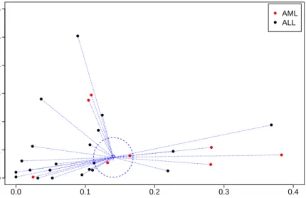
2.5.kNearest Neighbour 25 ? 0.0 0.1 0.2 0.3 0.4 0.0 0.1 0.2 0.3 0.4 0.5 0.6 ‘J03909_at’ Probset ‘M21005_at’ Probset AML ALL
Figure 2.3: k-nearest neighbour framework in a2-dimensional feature space for ‘Leukaemia’ dataset. Blue lines represent the Euclidian distances from the test observation, depicted by ‘?’ symbol, to all the training observations belonging to two classes: Acute Myeloid Leukemia (AML) shown in red dots; Acute Lymphoblast Leukemia (ALL) shown in black dots. For k=3, the nearest neighbours are identified within the dashed circle and the test observation is assigned to ‘AML’ class as the majority of the nearest observations
are the distance metric and the chosen value ofk(Ghosh et al. 2005).
The general framework of a kNN classifier in 2-dimensional setting is shown in
Fig-ure 2.3. From the ‘Leukaemia’ dataset (described in Appendix A.2), a subset of observations
whose gene expressions fall within a particular domain in respect with the considered
fea-ture space is shown in Figure 2.3. Two feafea-tures (genes), ‘J03909_at’ and ‘M21005_at’, are
represented on the horizontal and vertical axes respectively. The patients that represent
the training observations belong to one of two types of Leukaemia, either Acute Myeloid
Leukemia (AML) or Lymphoblast Leukemia (ALL). The test observation, denoted by ‘?’
symbol, is classified to the class of the majority in their neighbourhood. Euclidian distances
for the test observation (point) are measured from all given training observations. Then its
2.5.kNearest Neighbour 26
observation is assigned to the popular class in its neighbourhood which is ‘AML’.
General Rule of
k
Nearest Neighbour Classifier
According to thekNN rule, an unclassified (test) observation,xnew, is assigned to the class
label, ˆynew, of majority in itsknearest neighbours among the training dataset, where ˆynew =c
and c ∈ {1, . . . , C}. Although classification is the primary application of kNN, it can be also used for density estimation.
Thekdata points in the feature space lying within the neighbourhood of an observation
xnew are used to estimate the density function at xnew. The neighbourhood is identified
using a form of distance measure. A sphere (circle in two dimensional settings) centered
atxnew capturing thektraining points of this neighbourhood, irrespective of their classes,
is drawn. The estimated density atxnewcan be defined as:
ˆ
p(xnew)= k
νN , (2.11)
whereνdenotes the volume (area) of the sphere (circle). When the density atxnew is high,
thenkpoints can be quickly found as they are intuitively close toxnew. Hence, the volume
of the required sphere is small and then the obtained density, according to (2.11), is high.
On the other hand, when the density is low then the volume of the sphere required to
encompassknearest neighbours is large which leads to obtain a low density from (2.11).
Therefore, the density is mainly influenced by ν which performs a similar role to the
2.6. Support Vector Machine 27
The estimated conditional density ofxnew given a classccan be similarly defined as:
ˆ pxnew ynew =c = kc νNc , (2.12)
wherekcandNcdenote number of observations from thecth class that are involved within
the sphere and the entire training data respectively, such thatk= C P c=1 kc andN = C P c=1 Nc. The
estimator of class prior probability denoted by ˆπis given by:
ˆ
π=p yˆ new =c= Nc
N. (2.13)
Using Bayes rule, the posterior probability for class membership of the test observation
xnewcan be expressed by combining (2.11)-(2.13) as follows:
ˆ p ynew=c|xnew= ˆ pxnew ynew =c ·p yˆ new=c ˆ p(xnew) = kc νNc · Nc N k νN = kc k. (2.14)
The test observation is assigned to the class label c that has the largest fraction of the
observations belonging tocamong theknearest neighbours of the test observation (Bishop
et al. 2006).
2.6
Support Vector Machine
One of the most common classifiers is the Support Vector Machine (SVM). It is a well-known
supervised learning model in which training observations are used to recognize a pattern
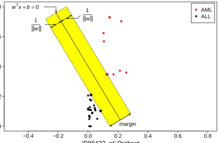
2.6. Support Vector Machine 28 −0.4 −0.2 0.0 0.2 0.4 0.6 0.8 0.0 0.2 0.4 0.6 0.8 ‘D88422_at’ Probset ‘X95735_at’ Probset margin wTx+b=0 1 ||w|| 1 ||w|| AML ALL
Figure 2.4: Support vector classifier in a2-dimensional feature space for the ‘Leukaemia’ dataset with a two linearly separable classes: Acute Myeloid Leukemia (AML) shown in red dots; Acute Lymphoblast Leukemia (ALL) shown in black dots. The hyperplane (line, in2-dimensional setting) of the decision boundary is the solid line, while dashed lines bound the shaded maximal margin of width2/kwk. The points highlighted by blue circles that lie on the margin boundaries are called ‘support vectors’.
hyperplane that separates ‘optimally’ the feature space into two disjoint regions such that
training observations of separate classes are divided by this hyperplane into two groups
with a ‘margin’ that is as maximum as possible.
For situations of linearly separable classes as illustrated by Figure 2.4, the main goal is
to design a hyperplane
f(x)=wTx+b=0 (2.15)
that classifies correctly all the training observations. A classification rule that associated
with this hyperplane can then be given by
fSVM(X)=sign
h
2.6. Support Vector Machine 29
It can be shown thatwTx
j+bgives the signed distance from a point xj to the hyperplane
defined in (2.15). Since the classes are linearly separable, one can find a hyperplane f (x),
as shown in (2.15), such that yj. f
xj
> 0 ∀j where yj ∈ {−1,1}. Such a hyperplane is
not unique (Vapnik & Vapnik 1998). The best solution is the one that has the maximum
‘margin’ between the training observations from different classes, see Figure 2.4.
The Optimization Problem
For simplicity, the vectorwis normalized so that
w Tx sv+b =1 (2.17)
wherexsvis a support vector for the assigned hyperplane. Since,wis a perpendicular vector
on the hyperplane in (2.15), the Euclidean distance from the hyperplane to its support vector
is the projection of the vector xsv−x on w, where x can be any point on the hyperplane wTx+b= 0. The margin is defined as the double of this distance. Therefore, the assigned
margin can be defined as
margin=2. w kwk.(xsv−x) , = 2 kwk w Tx sv+b− wTx+b = 2 kwk. (2.18)
The margin in (2.18) is obtained by applying the expressions shown in (2.15) and (2.17).
Now, the following optimization problem should be considered in order to assign a
2.6. Support Vector Machine 30 minimize 12wTw subject to yj wTx j+b ≥1, j= 1, . . . ,N, w∈RP, b ∈R. (2.19)
This problem is quadratic with linear inequality constraints. Therefore, it is a convex
optimization problem that can be solved by quadratic programming by means of Lagrange
multipliers (Vapnik & Vapnik 1998). The corresponding Lagrange (primal) function using
Karush-Kuhn-Tucker (KKT) approach (Boyd & Vandenberghe 2009) can be expressed as
L(w,b, α)= 1 2w Tw − N X j=1 αjyj wTxj+b −1 (2.20)
which is minimized with respect towandbsuch thatαj ≥0, whereαrepresents the vector of Lagrange multipliers,α∈RN. Setting the respective derivatives to zero results in
w= N X j=1 αjyjxj, (2.21) N X j=1 αjyj =0. (2.22)
By substituting (2.21) and (2.22) into (2.20), the Lagrange (dual) objective function can be
given by L(α)= N X j=1 αj− 1 2 N X j=1 N X l=1 αjαl yjyl xTjxl. (2.23)
TheL(α) in (2.23) is maximized with respect toαsubject toαj ≥0 and (2.22), j=1, . . . ,N. In addition to (2.21) and (2.22), the KKT conditions include the constraint
αjyj
wTxj+b
2.6. Support Vector Machine 31
These constraints uniquely characterize the solution to the primal and dual problem. In
view of (2.17) and (2.24), it can be shown thatαj >0 for support vectors (i.e., for eachxsv),
whereasαj =0 for the other training observations.
SVM provides a procedure that can control its sensitivity to potential outliers when the
considered datasets are noisy. When the feature space has no linear separation between
observations from different classes, SVM introduces slack variables that allow the margin to be violated. Such a margin is called “soft margin” (Vapnik & Vapnik 1998).
For non-linearly separable situations, SVM can perform classification efficiently by transforming the original feature space, X, into another space Z, usually with higher
di-mensions, using a function called the ‘kernel’. The optimization problem can be expressed
in a way that only involves the input features via inner products. Therefore, transformed
feature vectors zj for the input feature vectors xj are considered and the corresponding
Lagrange dual function in (2.23) is expressed in the form
L(α)= N X j=1 αj− 1 2 N X j=1 N X l=1 αjαl yjyl zTjzl. (2.25) where zT
jzl is the transformed inner product using the kernel functionK
xj, xl
. Hence,
the transformed space, Z, is not required at all, but we require only the kernel function
which produces the inner products in the transformed space,zT
jzl. A valid kernel should
2.7. Classifier Performance Evaluation via Cross Validation 32
for kernel function in the SVM literature are
Qth−Degree polynomial: Kxj, xl =1+xTjxl Q , Radial basis: Kxj, xl =exp −γ xj−xl 2 . (2.26)
2.7
Classifier Performance Evaluation via Cross Validation
A main task in a pattern recognition problem is the assessment of the model performance
and its generalization for new data. Ideally the accuracy of a classifier should be assessed
on an independent data, called the test dataset, while the classification rule is built on other
data, called the training dataset. However, in many real world problems (e.g., experiments
of microarray gene expressions), limited observations are available and both modelling
and assessment of the model are performed on these limited data. A classifier accuracy
calculated from the same training dataset leads to underestimate the true or generalized
error rate as the classifier is assessed on the same data that is used to fit it, and thereby
giving an optimistic measure for the error rate. Various approaches have been proposed
to deal with the problem of classification error estimation. The error of a classifier can
be expressed in terms of two factors, i.e. bias and variance (Kim 2009). One of the most
commonly and effectively used approaches is the cross validation technique.
Cross-Validation Method
The cross validation (C.V.) technique is the simplest method used for error estimation. It
copes with the problem of limiting availability of observations by using a portion of the
2.8. Summary 33
model. For instance in F-fold cross validation setting, the data is divided intoF folds of
approximately the same size. Afterwards, F−1 folds are used for fitting the model and one fold is used for testing the model performance. The process is performedFtimes with
different fold at each time. TheFestimates of misclassification error rates are then averaged to obtain a single estimate for the classifier error. Small values ofFresult in highly biased
estimators. On the other hand, large values ofFlead to more computationally expensive
estimators with a high variance. The special case of F = N, also known as leave one out cross validation, implies one observation is used for testing and N−1 observations are used for building the classifier. This setting of C.V. gives an unbiased estimator with high
variance (Friedman et al. 2001).
2.8
Summary
A statistical learning approach can be used to model and understand complex datasets.
By mapping the relationship between a set of features and a considered response, it can
build a predictive model based on a given training data. Based on how the training data
is presented, the learning process is described as either supervised, when a set of features
along-with supervised output labels (response) are trained, or unsupervised, when the
training data contains only the feature matrix.
Supervised ensemble learning trains multiple base models (classifiers) designed for
the same task by combining their predictions into a single ensemble classifier. CART
are considered base classifiers for most of the ensemble learning methods (e.g., Random
2.8. Summary 34
feature space into two disjoint regions.
Three different classifiers are described in this chapter: Random Forest (RF);kNearest Neighbour (kNN); Support Vector Machine (SVM).
RF classifier is an ensemble of trees that are constructed using different bootstrap sam-ples of the dataset. Unlike CART, each node is split using the best among a randomly
chosen subset of features.
kNN uses the training dataset with a nearest neighbour rule to classify an observation
to a target class c. A set of ktraining observations that are closest to the test observation
in the feature space are sorted out and then the test observation is classified to the class of
majority in theseknearest observations.
SVM uses the training observations to recognize a pattern that can predicts the classes
of new (unseen) data. An SVM model is a representation of a hyperplane that separates
‘optimally’ the feature space into two disjoint regions such that the training observations
of separate classes are divided by this hyperplane into two groups with a ‘margin’ that is
as maximum as possible.
Evaluation of a model’s performance can be accomplished by estimating its
misclassifi-cation error rate on a test dataset. One of the most common technique for error estimation
is the cross validation method. It uses a portion of the given dataset to fit the classification
model, whilst the remaining part is used for testing the model. It copes with the problem
of limiting availability of observations in most microarray gene expressions datasets.
The next chapter will describe various techniques for feature selection. Identification of
the relevant and informative features required for classification within functional genomic