Beyond comparisons of means: understanding changes in gene expression at the single cell level

M E T H O D

Open Access

Beyond comparisons of means:

understanding changes in gene expression

at the single-cell level

Catalina A. Vallejos

, Sylvia Richardson

and John C. Marioni

Abstract

Traditional differential expression tools are limited to detecting changes in overall expression, and fail to uncover the rich information provided by single-cell level data sets. We present a Bayesian hierarchical model that builds upon BASiCS to study changes that lie beyond comparisons of means, incorporating built-in normalization and quantifying technical artifacts by borrowing information from spike-in genes. Using a probabilistic approach, we highlight genes undergoing changes in cell-to-cell heterogeneity but whose overall expression remains unchanged. Control experiments validate our method’s performance and a case study suggests that novel biological insights can be revealed. Our method is implemented in R and available at https://github.com/catavallejos/BASiCS.

Keywords: Single-cell RNA-seq, Differential expression, Cellular heterogeneity

Background

The transcriptomics revolution – moving from bulk sam-ples to single-cell (SC) resolution – provides novel insights into a tissue’s function and regulation. In particular, single-cell RNA sequencing (scRNA-seq) has led to the identification of novel sub-populations of cells in multi-ple contexts [1–3]. However, compared to bulk RNA-seq, a critical aspect of scRNA-seq data sets is an increased cell-to-cell variability among the expression counts. Part of this variance inflation is related to biological differ-ences in the expression profiles of the cells (e.g., changes in mRNA content and the existence of cell sub-populations or transient states), which disappears when measuring bulk gene expression as an average across thousands of cells. Nonetheless, this increase in variability is also due in part totechnical noisearising from the manipulation of small amounts of starting material, which is reflected in weak correlations between technical replicates [4]. Such technical artifacts are confounded with genuine transcrip-tional heterogeneity and can mask the biological signal.

*Correspondence: [email protected]; [email protected]; [email protected]

1MRC Biostatistics Unit, Cambridge Institute of Public Health, Cambridge, UK 2EMBL European Bioinformatics Institute, Wellcome Trust Genome Campus, Cambridge, UK

Full list of author information is available at the end of the article

Among others, one objective of RNA-seq experiments is to characterize transcriptional differences between pre-specified populations of cells (given by experimental con-ditions or cell types). This is a key step for understanding a cell’s fate and functionality. In the context of bulk RNA-seq, two popular methods for this purpose are edgeR [5] and DESeq2 [6]. However, these are not designed to cap-ture feacap-tures that are specific to scRNA-seq data sets. In contrast, SCDE [7] has been specifically developed to deal with scRNA-seq data sets. All of these meth-ods target the detection ofdifferentially expressed genes based on log-fold changes (LFCs) of overall expression between the populations. However, restricting the anal-ysis to changes in overall expression does not take full advantage of the rich information provided by scRNA-seq. In particular – and unlike bulk RNA-seq – scRNA-seq can also reveal information about cell-to-cell expression heterogeneity. Critically, traditional approaches will fail to highlight genes whose expression is less stable in any given population but whose overall expression remains unchanged between populations.

More flexible approaches, capable of studying changes that lie beyond comparisons of means, are required to characterize differences between distinct populations of cells better. In this article, we develop a quantitative

method to fill this gap, allowing the identification of genes whose cell-to-cell heterogeneity pattern changes between pre-specified populations of cells. In particular, genes with less variation in expression levels within a spe-cific population of cells might be under more stringent regulatory control. Additionally, genes having increased biological variability in a given population of cells could suggest the existence of additional sub-groups within the analyzed populations. To the best of our knowl-edge, this is the first probabilistic tool developed for this purpose in the context of scRNA-seq analyses. We demonstrate the performance of our method using con-trol experiments and by comparing expression patterns of mouse embryonic stem cells (mESCs) between different stages of the cell cycle.

Results and discussion

A statistical model to detect changes in expression patterns for scRNA-seq data sets

We propose a statistical approach to compare expression patterns between P pre-specified populations of cells. It builds upon BASiCS [8], a Bayesian model for the analysis of scRNA-seq data. As in traditional differential expression analyses, for any given genei, changes in over-all expression are identified by comparing population-specific expression rates μ(_ip) (p = 1,. . .,P), defined as the relative abundance of gene i within the cells in populationp. However, the main focus of our approach is to assess differences in biological cell-to-cell hetero-geneity between the populations. These are quantified through changes in population- and gene-specific bio-logical over-dispersion parameters δ_i(p) (p = 1,. . .,P), designed to capture residual variance inflation (after nor-malization and technical noise removal) while attenuating the well-known confounding relationship between mean and variance in count-based data sets [9] (a similar con-cept was defined in the context of bulk RNA-seq by [10], using the termbiological coefficient of variation). Impor-tantly, such changes cannot be uncovered by standard differential expression methods, which are restricted to changes in overall expression. Hence, our approach pro-vides novel biological insights by highlighting genes that undergo changes in cell-to-cell heterogeneity between the populations despite the overall expression level being pre-served.

To disentangle technical from biological effects, we exploit spike-in genes that are added to the lysis buffer and thence theoretically present at the same amount in every cell (e.g., the 92 ERCC molecules developed by the External RNA Control Consortium [11]). These provide an internal control or gold standard to estimate the strength of technical variability and to aid normaliza-tion. In particular, these control genes allow inference on

cell-to-cell differences in mRNA content, providing additional information about the analyzed populations of cells [12]. These are quantified through changes between cell-specific normalizing constants φ_j(p) (for the jth cell within the pth population). Critically, as described in Additional file 1: Note S1 and Fig. S1, global shifts in mRNA content between populations do not induce spurious differences when comparing gene-specific parameters (provided the offset correction described in ‘Methods’ is applied).

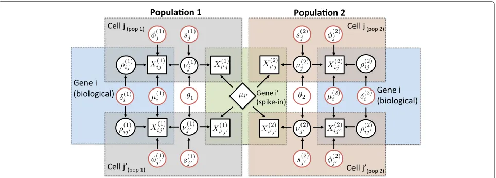
A graphical representation of our model is displayed in Fig. 1 (based on a two-group comparison). It illustrates how our method borrows information across all cells and genes (biological transcripts and spike-in genes) to per-form inference. Posterior inference is implemented via a Markov chain Monte Carlo (MCMC) algorithm, gener-ating draws from the posterior distribution of all model parameters. Post-processing of these draws allows quan-tification of supporting evidence regarding changes in expression patterns (mean and over-dispersion). These are measured using a probabilistic approach based on tail posterior probabilities associated with decision rules, where a probability cut-off is calibrated through the expected false discovery rate (EFDR) [13].

Our strategy is flexible and can be combined with a variety of decision rules, which can be altered to reflect the biological question of interest. For example, if the aim is to detect genes whose overall expression changes between populationspandp, a natural decision rule is |log(μ(_ip)/μ_i(p))| > τ0, where τ0 ≥ 0 is an a priori

cho-sen biologically significant threshold for LFCs in overall expression, to avoid highlighting genes with small changes in expression that are likely to be less biologically relevant [6, 14]. Alternatively, changes in biological cell-to-cell het-erogeneity can be assessed using |log(δ(_ip)/δ_i(p))| > ω0,

for a given minimum tolerance thresholdω0 ≥0. This is

the main focus of this article. As a default option, we sug-gest settingτ0= ω0=0.4, which roughly coincides with

a 50 % increase in overall expression or over-dispersion in whichever group of cells has the largest value (this choice is also supported by the control experiments shown in this article). To improve the interpretation of the genes high-lighted by our method, these decision rules can also be complemented by, e.g., requiring a minimum number of cells where the expression of a gene is detected.

More details regarding the model setup and the implementation of posterior inference can be found in ‘Methods’.

Alternative approaches for identifying changes in mean expression

Fig. 1Graphical representation of our model for detecting changes in expression patterns (mean and over-dispersion) based on comparing two predefined population of cells. The diagram considers expression counts of two genes (iis biological andiis technical) and two cells (jpandjp) from

each populationp₌1, 2. Observed expression counts are represented bysquare nodes. The centralrhomboid nodedenotes the known input number of mRNA molecules for a technical genei, which is assumed to be constant across all cells. The remainingcircular nodesrepresent unknown elements, usingblackto denote random effects andredto denote model parameters (fixed effects) that lie on the top of the model’s hierarchy. Here,φ(_jp)’s ands(_jp)’s act as normalizing constants that are cell-specific andθp’s are global over-dispersion parameters capturing technical variability,

which affect the expression counts of all genes and cells within each population. In this diagram,ν_j(p)’s andρ(_ijp)’s represent random effects related to

technical and biological variability components, whose variability is controlled by_θp’s andδ(ip)’s, respectively (see Additional file 1: Note 6.1). Finally,

μ(p) i ’s andδ(

p)

i ’s, respectively, measure the overall expression of a geneiand its residual biological cell-to-cell over-dispersion (after normalization,

technical noise removal and adjustment for overall expression) within each population. Colored areas highlight elements that are shared within a gene and/or cell. The latter emphasizes how our model borrows information across all cells to estimate parameters that are gene-specific and all genes to estimate parameters that are cell-specific. More details regarding the model setup can be found in the ‘Methods’ section of this article

RNA-seq literature (e.g., DESeq2 [6] and edgeR [5]). However, such methods are not designed to cap-ture feacap-tures that are specific to SC-level experiments (e.g., the increased levels of technical noise). Instead, BASiCS, SCDE [7] and MAST [15] have been specifi-cally developed with scRNA-seq data sets in mind. SCDE is designed to detect changes in mean expression while accounting fordropout events, where the expression of a gene is undetected in some cells due to biological variability or technical artifacts. For this purpose, SCDE employs a two-component mixture model where nega-tive binomial and low-magnitude Poisson components model amplified genes and the background signal related todropoutevents, respectively. MAST is designed to cap-ture more complex changes in expression, using a hurdle model to study both changes in the proportion of cells where a gene is expressed above background and in the positive expression mean, defined as a conditional value – given than the gene is expressed above background levels. Additionally, MAST uses the fraction of genes that are detectably expressed in each cell (the cellular detection rate or CDR) as a proxy to quantify technical and bio-logical artifacts (e.g., cell volume). SCDE and MAST rely on pre-normalized expression counts. Moreover, unlike BASiCS, SCDE and MAST use a definition of changes

in expression mean that is conceptually different to what would be obtained based on a bulk population (which would consider all cells within a group, regardless of whether a gene is expressed above background or not).

The performance of these methods is compared in Additional file 1: Note S2 using real and simulated data sets. While control of the false discovery rate (FDR) is not well calibrated for BASiCS when setting τ0 = 0, this control is substantially improved when

increasing the LFC threshold to τ0 = 0.4 – which

Alternative approaches for identifying changes in heterogeneity of expression

To the best of our knowledge, BASiCS is the first prob-abilistic tool to quantify gene-specific changes in the variability of expression between populations of cells. Instead, previous literature has focused on compar-isons based on the coefficient of variation (CV), calcu-lated from pre-normalized expression counts (e.g., [17]), for which no quantitative measure of differential vari-ability has been obtained. More recently, [9] proposed a mean-corrected measure of variability to avoid the confounding effect between mean expression and CV. Nonetheless, the latter was designed to compare expres-sion patterns for sets of genes, rather than for individual genes.

Not surprisingly, our analysis suggests that a quantification of technical variability is critical when comparing variability estimates between cell populations (Additional file 1: Note S3 and Fig. S5). In particular, comparisons based on CV estimates can mask the bio-logical signal if the strength of technical variability varies between populations.

A control experiment: comparing single cells vs pool-and-split samples

To demonstrate the efficacy of our method, we use the control experiment described in [17], where sin-gle mESCs are compared against pool-and-split (P&S) samples, consisting of pooled RNA from thousands of mESCs split into SC equivalent volumes. Such a con-trolled setting provides a situation where substantial changes in overall expression are not expected as, on average, the overall expression of SCs should match the levels measured in P&S samples. Additionally, the

design of P&S samples should remove biological variation, leading to a homogeneous set of samples. Hence, P&S samples are expected to show a genuine reduc-tion in biological cell-to-cell heterogeneity compared to SCs.

Here, we display the analysis of samples cultured in a 2i media. Hyper-parameter values forμ(_ip)’s andδ(_ip)’s were set toa2_μ = a2_δ = 0.5, so that extreme LFC estimates are shrunk towards(−3, 3)(see ‘Methods’). However, varying a2

μ anda2δ leads to almost identical results (not shown), suggesting that posterior inference is in fact dominated by the data. In these data, expression counts correspond to the number of molecules mapping to each gene within each cell. This is achieved by using unique molecular identifiers (UMIs), which remove amplification biases and reduce sources of technical variation [18]. Our analysis includes 74 SCs and 76 P&S samples (same inclusion cri-teria as in [17]) and expression counts for 9378 genes (9343 biological and 35 ERCC spikes) defined as those with at least 50 detected molecules in total across all cells. The R code used to perform this analysis is provided in Additional file 2.

To account for potential batch effects, we allowed different levels of technical variability to be estimated in each batch (see Additional file 1: Note S4 and Fig. S6). Moreover, we also performed an independent analysis of each batch of cells. As seen in Additional file 1: Fig. S7, the results based on the full data are roughly replicated in each batch, suggesting that our strategy is able to remove potential artifacts related to this batch effect.

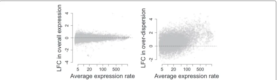
As expected, our method does not reveal major changes in overall expression between SCs and P&S samples as the distribution of LFC estimates is roughly symmetric with respect to the origin (see Fig. 2a) and the majority of genes

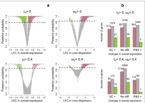
are not classified as differentially expressed at 5 % EFDR (see Fig. 3b). However, this analysis suggests that setting the minimum LFC tolerance thresholdτ0equal to 0 is too

liberal as small LFCs are associated with high posterior probabilities of changes in expression (see Fig. 3a) and the number of differentially expressed genes is inflated (see Fig. 3b). In fact, counter-intuitively, 4710 genes (≈50 % of all analyzed genes) are highlighted to have a change in overall expression when using τ0 = 0. This is

par-tially explained by the high nominal FDR rates displayed in Additional file 1: Note S2.1 where, forτ0 = 0, FDR is

poorly calibrated when simulating under the null model. In addition, we hypothesize this heavy inflation is also due

to small but statistically significant differences in expres-sion that are not biologically meaningful. In fact, the num-ber of genes whose overall expression changes is reduced to 559 (≈6 % of all analyzed genes) when settingτ0 =

0.4. As discussed earlier, this minimum threshold roughly coincides with a 50 % increase in overall expression and with the 90th percentile of empirical LFC estimates when simulating under the null model (no changes in expression). Posterior inference regarding biological over-dispersion is consistent with the experimental design, where the P&S samples are expected to have more homogeneous expression patterns. In fact, as shown in Fig. 2b, the distribution of estimated LFCs in biological

a

b

over-dispersion is skewed towards positive values (higher biological over-dispersion in SCs). This is also supported by the results shown in Fig. 3b, where slightly more than 2000 genes exhibit increased biological over-dispersion in SCs and almost no genes (≈60 genes) are high-lighted to have higher biological over-dispersion in the P&S samples (EFDR = 5 %). In this case, the choice of ω0 is less critical (within the range explored here).

This is illustrated by the left panels in Fig. 3a, where tail posterior probabilities exceeding the cut-off defined by EFDR = 5 % correspond to similar ranges of LFC estimates.

mESCs across different cell-cycle stages

Our second example shows the analysis of the mESC data set presented in [16], which contains cells where the cell-cycle phase is known (G1, S and G2M). After applying the same quality control criteria as in [16], our analy-sis considers 182 cells (59, 58 and 65 cells in stages G1, S and G2M, respectively). To remove genes with consis-tently low expression across all cells, we excluded those genes with less than 20 reads per million (RPM), on aver-age, across all cells. After this filter, 5,687 genes remain (including 5,634 intrinsic transcripts, and 53 ERCC spike-in genes). The R code used to perform this analysis is provided in Additional file 3.

As a proof of concept, to demonstrate the effi-cacy of our approach under a negative control, we performed permutation experiments, where cell labels were randomly permuted into three groups (containing 60, 60 and 62 samples, respectively). In this case, our method correctly infers that mRNA content as well as gene expression profiles do not vary across groups of randomly permuted cells (Fig. 4).

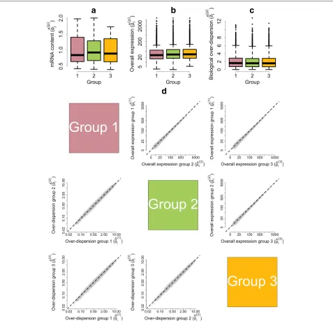
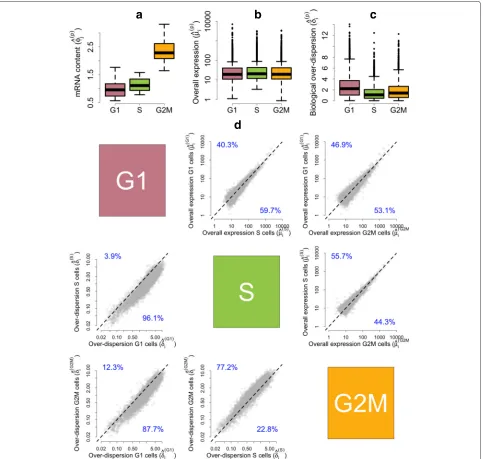
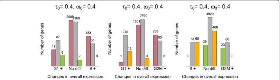
As cells progress through the cell cycle, cellular mRNA content increases. In particular, our model infers that mRNA content is roughly doubled when comparing cells in G1 vs G2M, which is consistent with the duplication of genetic material prior to cell division (Fig. 5a). Our analysis suggests there are no major shifts in expression levels between cell-cycle stages (Fig. 5b and upper tri-angular panels in Fig. 5d). Nonetheless, a small number of genes are identified as displaying changes in over-all expression between cell-cycle phases at 5 % EFDR for τ0 = 0.4 (Fig. 6). To validate our results, we

per-formed gene ontology (GO) enrichment analysis within those genes classified as differentially expressed between cell-cycle phases (see Additional file 3). Not surprisingly, we found an enrichment of mitotic genes among the 545 genes classified as differentially expressed between G1 and G2M cells. In addition, the 209 differentially expressed genes between S and G2M are enriched for regulators of cytokinesis, which is the final stage of the

cell cycle where a progenitor cell divides into two daughter cells [19].

Our method suggests a substantial decrease in biolog-ical over-dispersion when cells move from G1 to the S phase, followed by a slight increase after the transition from S to the G2M phase (see Fig. 5c and the lower trian-gular panels in Fig. 5d). This is consistent with the findings in [19], where the increased gene expression variability observed in G2M cells is attributed to an unequal distri-bution of genetic material during cytokinesis and the S phase is shown to have the most stable expression patterns within the cell cycle. Here, we discuss GO enrichment of those genes whose overall expression rate remains con-stant (EFDR = 5 %, τ0 = 0.4) but that exhibit changes

in biological over-dispersion between cell-cycle stages (EFDR=5 %,ω0 = 0.4). Critically, these genes will not

be highlighted by traditional differential expression tools, which are restricted to differences in overall expression rates. For example, among the genes with higher biologi-cal over-dispersion in G1 with respect to the S phase, we found an enrichment of genes related to protein dephos-phorylation. These are known regulators of the cell cycle [20]. Moreover, we found that genes with lower biologi-cal over-dispersion in G2M cells are enriched for genes related to DNA replication checkpoint regulation (which delays entry into mitosis until DNA synthesis is completed [21]) relative to G1 cells and mitotic cytokinesis when comparing to S cells. Both of these processes are likely to be more tightly regulated in the G2M phase. A full table with GO enrichment analysis of the results described here is provided in Additional file 3.

Conclusions

a

b

c

d

Fig. 4Posterior estimates of model parameters based on random permutations of the mESC cell-cycle data set. For a single permuted data set:

aEmpirical distribution of posterior medians for mRNA content normalizing constants_φjpacross all cells.bEmpirical distribution of posterior medians for gene-specific expression rates_μipacross all genes.cEmpirical distribution of posterior medians for gene-specific biological

over-dispersion parameters_δipacross all genes.dAs an average across ten random permutations.Upper diagonal panelscompare estimates for

gene-specific expression rates_μipbetween groups of cells.Lower diagonal panelscompare gene-specific biological over-dispersion parametersδip

between groups of cells

is broken when analyzing heterogeneous populations, see Section S8 in [8]). This is illustrated in Additional file 1: Note S5 using the cell-cycle data set analyzed here (Additional file 1: Figs. S8 and S9). Due to this interplay between overall expression and over-dispersion, the interpretation of over-dispersion parameters δ_i(p) requires careful consideration. In particular, it is not

trivial to interpret differences between δ_i(p)’s when the μ(p)

i ’s also change. As a consequence, our analysis focuses

a

b

d

c

Fig. 5Posterior estimates of model parameters for mESCs across different cell-cycle phases.aEmpirical distribution of posterior medians for mRNA content normalizing constantsφ(_jp)across all cells.bEmpirical distribution of posterior medians for gene-specific expression ratesμ(_ip)across all genes.cEmpirical distribution of posterior medians for gene-specific biological over-dispersion parameters_δ(_ip)across all genes.dUpper diagonal panelscompare estimates for gene-specific expression ratesμ(_ip)between groups of cells.Lower diagonal panelscompare gene-specific biological over-dispersion parametersδ_i(p)between groups of cells. While our results suggest there are no major shifts in mean expression between cell-cycle stages, our results suggest a substantial decrease in biological over-dispersion when cells move from G1 to the S phase, followed by a slight increase after the transition from S to the G2M phase (to give a rough quantification of this statement, panel (d) includes the percentage of point estimates that lie on each side of thediagonal line)

A decision rule to determine changes in expression patterns is defined through a probabilistic approach based on tail posterior probabilities and calibrated using the EFDR. The performance of our method was demonstrated using a controlled experiment where we

recovered the expected behavior of gene expression patterns.

Fig. 6Summary of changes in expression patterns (mean and over-dispersion) for the mESC cell-cycle data set (EFDR₌5 %). Bins in the horizontal axis summarize changes in overall expression between each pair of groups. We use G1+, S+ and G2M+ to denote that higher overall expression was detected in cell-cycle phase G1, S and G2M, respectively [the central group ofbars(No diff.) corresponds to those genes where no significant differences were found].Colored barswithin each group summarize changes in biological over-dispersion between the groups. We usepink,green andyellow barsto denote higher biological over-dispersion in cell-cycle phases G1, S and G2M, respectively (andgrayto denote no significant differences were found). The numbers of genes are displayed in log-scale

expression of a gene is only detected in a small proportion of cells (e.g., high expression in a handful of cells but no expression in the remaining cells). These situations will be reflected in low and high estimates of δ(_ip), respec-tively. However, the biological relevance of these estimates is not clear. Hence, to improve the interpretation of the genes highlighted by our method, we suggest comple-menting the decision rules presented here by conditioning the results of the test on a minimum number of cells where the expression of a gene is detected.

Currently, our approach requires predefined popula-tions of cells (e.g., defined by cell types or experimen-tal conditions). However, a large number of scRNA-seq experiments involve a mixed population of cells, where cell types are not known a priori (e.g., [1–3]). In such cases, expression profiles can be used to cluster cells into distinct groups and to characterize markers for such sub-populations. Nonetheless, unknown group structures introduce additional challenges for normalization and quantification of technical variability since, e.g., noise levels can vary substantially between different cell popu-lations. A future extension of our work is to combine the estimation procedure within our model with a clustering step, propagating the uncertainty associated with each of these steps into downstream analysis. In the meantime, if the analyzed population of cells contains a sub-population structure, we advise the user to cluster cells first (e.g., using a rank-based correlation, which is more robust to normalization), thus defining groups of cells that can be used as an input for BASiCS. This step will also aid the interpretation of model parameters that are gene-specific. Until recently, most scRNA-seq data sets consisted of hundreds (and sometimes thousands) of cells. However, droplet-based approaches [22, 23] have recently allowed parallel sequencing of substantially larger numbers of cells

in an effective manner. This brings additional challenges to the statistical analysis of scRNA-seq data sets (e.g., due to the existence of unknown sub-populations, requiring unsupervised approaches). In particular, current proto-cols do not allow the addition of technical spike-in genes. As a result, the deconvolution of biological and techni-cal artifacts has become less straightforward. Moreover, the increased sample sizes emphasize the need for more computationally efficient approaches that are still able to capture the complex structure embedded within scRNA-seq data sets. To this end, we foresee the use of parallel programming as a tool for reducing computing times. Additionally, we are also exploring approximated poste-rior inference based, for example, on an integrated nested Laplace approximation [24].

Finally, our approach lies within a generalized linear mixed model framework. Hence, it can be easily extended to include additional information such as covariates (e.g., cell-cycle stage, gene length and GC content) and exper-imental design (e.g., batch effects) using fixed and/or random effects.

Methods

A statistical model to detect changes in expression patterns for scRNA-seq data sets

particularly critical when there are substantial differences in cellular mRNA content, amplification biases and other sources of technical variation. For this purpose, we exploit technical spike-in genes, which are added at the (theoreti-cally) same quantity to each cell’s lysate. A typical example is the set of 92 ERCC molecules developed by the External RNA Control Consortium [11]. Our method builds upon BASiCS [8] and can perform comparisons between multi-ple populations of cells using a single model. Importantly, our strategy avoids stepwise procedures where data sets are normalized prior to any downstream analysis. This is an advantage over methods using pre-normalized counts, as the normalization step can be distorted by technical artifacts.

We assume that there areP groups of cells to be com-pared, each containingnpcells (p=1,. . .,P). LetXij(p)be

a random variable representing the expression count of a gene i(i = 1,. . .,q) in the jth cell from groupp. With-out loss of generality, we assume the first q0 genes are

biological and the remainingq−q0are technical spikes.

Extending the formulation in BASiCS, we assume that

E

X_ij(p)

=

φ(p) j s

(p) j μ

(p)

i , i=1,. . .,q0;

s(_jp)μ(_ip), i=q0+1,. . .,q.

and (1)

CV2_X(p)

ij

=

(φ(p)

j s( p)

j μ( p)

i )−1+θp+δ(ip)(θp+1),i=1,. . .,q0;

(s(_jp)μ(_ip))−1_+θ

p, i=q0+1,. . .,q, (2)

with μ(_ip) ≡ μi for i = q0+ 1,. . .,q and where CV

stands forcoefficient of variation (i.e., the ratio between standard deviation and mean). These expressions are the result of a Poisson hierarchical structure (see Additional file 1: Note S6.1). Here, φ_j(p)’s act as cell-specific nor-malizing constants (fixed effects), capturing differences in input mRNA content across cells (reflected by the expression counts of intrinsic transcripts only). A second set of normalizing constants, s(_jp)’s, capture cell-specific scale differences affecting the expression counts of all genes (intrinsic and technical). Among others, these dif-ferences can relate to sequencing depth, capture efficiency and amplification biases. However, a precise interpreta-tion of thes(_jp)’s varies across experimental protocols, e.g., amplification biases are removed when using UMIs [18]. In addition, θp’s are global technical noise parameters

controlling the over-dispersion (with respect to Poisson sampling) of all genes within groupp. The overall expres-sion rate of a geneiin grouppis denoted byμ(_ip). These are used to quantify changes in the overall expression of a gene across groups. Similarly, theδ_i(p)’s capture residual over-dispersion (beyond what is due to technical artifacts) of every gene within each group. These so-called biolog-ical over-dispersion parameters relate to heterogeneous

expression of a gene across cells. For each group, stable housekeeping-like genes lead toδ(_ip) ≈ 0 (low residual variance in expression across cells) and highly variable genes are linked to large values ofδ_i(p). A novelty of our approach is the use ofδ_i(p)to quantify changes in biological over-dispersion. Importantly, this attenuates confounding effects due to changes in overall expression between the groups.

A graphical representation of this model is displayed in Fig. 1. To ensure identifiability of all model parameters, we assume thatμ(_ip)’s are known for the spike-in genes (and given by the number of spike-in molecules that are added to each well). Additionally, we impose the identifiability restriction

1 np

np

j=1

φ(p)

j =1, forp=1,. . .,P. (3)

Here, we discuss the priors assigned to parameters that are gene- and group-specific (see Additional file 1: Note S6.2 for the remaining elements of the prior). These are given by

μ(p) i

iid

∼log N0,a2_μ andδ_i(p)iid∼log N0,a2_δ fori=1,. . .,q0.

(4)

Hereafter, without loss of generality, we simplify our notation to focus on two-group comparisons. This is equivalent to assigning Gaussian prior distributions for LFCs in overall expression (τi) or biological

over-dispersion (ωi). In such a case, it follows that

τi≡log

μ(1)

i

μ(2)

i

∼ N0, 2a2_μ and

ωi≡log

δ(1)

i

δ(2)

i

∼ N0, 2a2_δ.

(5)

Hence, our prior is symmetric, meaning that we do not a priori expect changes in expression to be skewed towards either group of cells. Values for a2

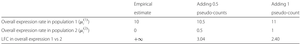
μ anda2δ can be elicited using an expected range of values for LFC in expression and biological over-dispersion, respectively. The latter is particularly useful in situations where a gene is not expressed (or very lowly expressed) in one of the groups, where, e.g., LFCs in overall expression are unde-fined (the maximum likelihood estimate of τi would be

±∞, the sign depending on which group expresses gene i). A popular solution to this issue is the addition of pseudo-counts, where an arbitrary number is added to all expression counts (in all genes and cells). This strategy is also adopted in models that are based on log-transformed expression counts (e.g., [15]). While the latter guaran-tees thatτiis well defined, it leads to artificial estimates

for τi (see Table 1). Instead, our approach exploits an

informative prior (indexed bya2

Table 1Synthetic example to illustrate the effect of addition of pseudo-counts over the estimation of LFCs in overall expression

Empirical Adding 0.5 Adding 1

estimate pseudo-counts pseudo-count

Overall expression rate in population 1 (μ(_i1)) 10 10.5 11

Overall expression rate in population 2 (μ(_i2)) 0 0.5 1

LFC in overall expression 1 vs 2 +∞ 3.04 2.40

For simplicity, we assume that normalization is not required so that pseudo-counts are linearly reflected in the overall expression rates. While pseudo-counts introduce an additive effect, LFC estimates measure changes on a multiplicative scale. Hence, addition of pseudo-counts leads to an artificial deflation of LFC estimates. As a consequence, such estimates cannot be meaningfully interpreted

to a meaningful shrinkage strength, which is based on prior knowledge. Importantly – and unlike the addition of pseudo-counts – our approach is also helpful when com-paring biological over-dispersion between the groups. In fact, if a geneiis not expressed in one of the groups, this will lead to a non-finite estimate of ωi (if all expression

counts in a group are equal to zero, the correspond-ing estimate of the biological over-dispersion parameters would be equal to zero). Adding pseudo-counts cannot resolve this issue, but imposing an informative prior forωi

(indexed bya2_ω) will shrink estimates towards the appro-priate range.

Generally, posterior estimates ofτiandωiare robust to

the choice of a2

μ anda2δ, as the data is informative and dominates posterior inference. In fact, these values are only influential when shrinkage is needed, e.g., when there are zero total counts in one of the groups. In such cases, posterior estimates ofτiandωiare dominated by the prior,

yet the method described below still provides a tool to quantify evidence of changes in expression. As a default option, we usea2_μ= a2_δ = 0.5 leading toτi,ωi ∼ N(0, 1).

These default values imply that approximately 99 % of the LFCs in overall expression and over-dispersion are expected a priori to lie in the interval(−3, 3). This range seems reasonable in light of the case studies we have explored. If a different range is expected, this can be easily modified by the user by setting different values fora2_μand a2_δ.

Posterior samples for all model parameters are gener-ated via an adaptive Metropolis within a Gibbs sampling algorithm [25]. A detailed description of our implementa-tion can be found in Addiimplementa-tional file 1: Note S6.3.

Post hoc correction of global shifts in input mRNA content between the groups

The identifiability restriction in Eq. 3 applies only to cells within each group. As a consequence, if they exist, global shifts in cellular mRNA content between groups (e.g., if all mRNAs were present at twice the level in one population related to another) are absorbed by theμ(_ip)’s. To assess changes in the relative abundance of a gene, we adopt a two-step strategy where: (1) model parameters are esti-mated using the identifiability restriction in Eq. 3 and (2)

global shifts in endogenous mRNA content are treated as a fixedoffset and corrected post hoc. For this purpose, we use the sum of overall expression rates (intrinsic genes only) as a proxy for the total mRNA content within each group. Without loss of generality, we use the first group of cells as a reference population. For each population p(p = 1,. . .,P), we define a population-specific offset effect:

p= q0

i=1

μ(p) i

q0

i=1

μ(1)

i

(6)

and perform the following offset correction:

˜ μ(p)

i =μ (p) i

p, φ˜(jp)=φ (p) j × p,

i=1,. . .,q0; jp=1,. . .,np.

(7)

This is equivalent to replacing the identifiability restric-tion in Eq. 3 by

1 np

np

j=1

φ(p)

j = p, forp=1,. . .,P. (8)

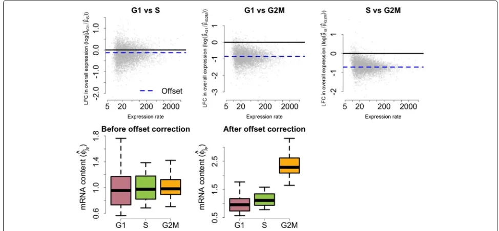
Technical details regarding the implementation of this post hoc offset correction are explained in Additional file 1: Note S6.4. The effect of this correction is illustrated in Fig. 7 using the cell-cycle data set described in the main text. As an alternative, we also explored the use of the ratio between the total intrinsic counts over total spike-in counts to define a similar offset correction based on

p=

⎛ ⎝median

j=1,...,np

⎧ ⎨ ⎩

q0

i=1X(

p)

ij

q i=q0+1X(

p) ij ⎫ ⎬ ⎭ ⎞

⎠ ⎛⎝median

j=1,...,n1 ⎧ ⎨ ⎩

q0

i=1X( 1)

ij

q i=q0+1X

(1)

ij ⎫ ⎬ ⎭ ⎞ ⎠. (9)

For the cell-cycle data set, both alternatives are equiva-lent. Nonetheless, the first option is more robust in cases where a large number of differentially expressed genes are present. Hereafter, we useμ(_ip)andφ_j(p)to denoteμ˜(_ip)and

˜ φ(p)

j , respectively.

A probabilistic approach to quantify evidence of changes in expression patterns

Fig. 7Post hoc offset correction for cell-cycle data set.Upper panelsdisplay posterior medians for LFC in overall expression against the weighted average between estimates of overall expression rates for G1, S and G2M cells (weights defined by the number of cells in each group).Lower panels illustrate the effect of the offset correction upon the empirical distribution of posterior estimates for mRNA content normalizing constantsφ(_jp). These figures illustrate a shift in mRNA content throughout cell-cycle phases. In particular, our model infers that cellular mRNA is roughly duplicated when comparing G1 to G2M cells.LFClog-fold change

simple and intuitive scale of evidence. Our strategy is flex-ible and can be combined with a variety of decision rules. In particular, here we focus on highlighting genes whose absolute LFC in overall expression and biological over-dispersion between the populations exceeds minimum tolerance thresholdsτ0andω0, respectively (τ0,ω0 ≥ 0),

set a priori. The usage of such minimum tolerance lev-els for LFCs in expression has also been discussed in [14] and [6] as a tool to improve the biological significance of detected changes in expression and to improve upon FDRs.

For a given probability thresholdαM (0.5 < αM < 1),

a gene i is identified as exhibiting a change in overall expression between populationspandpif

πM

ipp(τ0)≡P(|log(μ(ip)/μ (p)

i )|> τ0|{data}) > αM,

i=1,. . .,q0.

(10)

If τ0 → 0,πiM(τ0) → 1 becoming uninformative to

detect changes in expression. As in [26], in the limiting case whereτ0=0, we define

πM

ipp(0)=2 max

˜ πM

ipp, 1− ˜πippM

−1 (11)

with

˜ πM

ipp =P

logμ(_ip)/μ_i(p)>0| {data}. (12)

A similar approach is adopted to study changes in bio-logical over-dispersion between populations p and p, using

πD

ipp(ω0)≡P

|logδ_i(p)/δ_i(p)|> ω0|{data}

> αD,

(13)

for a fixed probability thresholdαD(0.5< αD <1). In line

with Eqs. 11 and 12, we also define

πD

ipp(0)=2 max

˜ πD

ipp, 1− ˜πippD

−1 (14)

with

˜ πD

ipp =P

logδ(_ip)/δ_i(p)>0| {data}. (15)

Evidence thresholds αM and αD can be fixed a priori.

Otherwise, these can be defined by controlling the EFDR [13]. In our context, these are given by

EFDRαM(τ0)=

q0

i=1

1−π_iM(τ0)

Iπ_iM(τ0) > αM

q0

i=1I

πM

i (τ0) > αM

(16)

and

EFDRαD(ω0)=

q0

i=1

1−π_iD(ω0)Iπ_iD(ω0) > αD

q0

i=1I

πD

i (ω0) > αD

,

where I(A) = 1 if eventAis true, 0 otherwise. Critically, the usability of this calibration rule relies on the existence of genes under both the null and the alternative hypoth-esis (i.e., with and without changes in expression). While this is not a practical limitation in real case studies, this calibration might fail to return a value in benchmark data sets (e.g., simulation studies), where there are no changes in expression. As a default, if EFDR calibration is not possible, we setαM =αD =0.90.

The posterior probabilities in Eqs. 10, 11, 13 and 14 can be easily estimated – as a post-processing step – once the model has been fitted (see Additional file 1: Note S6.5). In addition, our strategy is flexible and can be easily extended to investigate more complex hypothe-ses, which can be defined post hoc, e.g., to identify those genes that show significant changes in cell-to-cell biological over-dispersion but that maintain a con-stant level of overall expression between the groups, or conditional decision rules where we require a mini-mum number of cells where the expression of a gene is detected.

Software

Our implementation is freely available as an R package [27], using a combination of R and C++ functions through the Rcpp library [28]. This can be found in https://github. com/catavallejos/BASiCS, released under the GPL license.

Availability of supporting data

All data sets analyzed in this article are publicly available in the cited references.

Ethics

Not applicable.

Additional files

Additional file 1:Supplementary material. Section S1 illustrates the interaction between cell- and gene-specific model parameters. Section S2 provides a comparative analysis of BASiCS and alternative methods regarding the detection of differentially expressed genes (changes in mean). Section S3 illustrates the usage of the coefficient of variation as a measure of cellular heterogeneity. Section S4 describes the treatment of potential batch effects used for the analysis of the data set provided by [17]. Section S5 illustrates the interplay between mean and over-dispersion parameters that is typically observed in homogeneous populations of cells. Section S6 contains additional details regarding the statistical model presented in this article and the implementation of Bayesian inference. (PDF 1443 kb)

Additional file 2:Data analysis (part 1). R code used to analyze the single cells vs pool-and-split samples data set. (PDF 3952 kb)

Additional file 3:Data analysis (part 2). R code used to analyze the cell-cycle data set. (PDF 3051 kb)

Abbreviations

BASiCS, Bayesian analysis of single-cell sequencing data; bulk RNA-seq, bulk RNA sequencing; CDR, cellular detection rate; CV, coefficient of variation; EFDR, expected false discovery rate; ERCC, External RNA Control Consortium; FDR,

false discovery rate; GO, gene ontology; LFC, log-fold change; MCMC, Markov chain Monte Carlo; mESC, mouse embryonic stem cell; P&S, pool-and-split; SC, single cell; scRNA-seq, single-cell RNA sequencing; UMI, unique molecular identifier.

Competing interests

The authors declare that they have no competing interests.

Authors’ contributions

CAV, JCM and SR conceived and designed the methods and experiments. CAV implemented the methods and analyzed the data. All authors were involved in writing the paper and have approved the final version.

Acknowledgments

We acknowledge all members of the Richardson research group (Medical Research Council - Biostatistics Unit, MRC-BSU) and Marioni laboratory (European Molecular Biology Laboratory - European Bioinformatics Institute, EMBL-EBI; Cancer Research UK - Cambridge Institute, CRUK-CI) for support and discussions during the preparation of this document. In particular, we are grateful to Nils Eling (EMBL-EBI), Antonio Scialdone (EMBL-EBI) and Aaron Lun (CRUK-CI) for numerous discussions and suggestions that enriched the final version of the manuscript. We also thank the editorial team ofGenome Biology and two independent reviewers for the positive feedback and many insightful and constructive comments provided.

Funding

JCM and CAV acknowledge core EMBL funding. SR and CAV acknowledge core MRC funding (MRC_MC_UP_0801/1). JCM acknowledges core support from CRUK.

Author details

1_{MRC Biostatistics Unit, Cambridge Institute of Public Health, Cambridge, UK.} 2_{EMBL European Bioinformatics Institute, Wellcome Trust Genome Campus,}

Cambridge, UK.3_{Cancer Research UK Cambridge Institute, University of}

Cambridge, Li Ka Shing Centre, Cambridge, UK.

Received: 21 December 2015 Accepted: 30 March 2016

References

1. Zeisel A, Muñoz-Manchado AB, Codeluppi S, Lönnerberg P, La Manno G, Juréus A, et al. Cell types in the mouse cortex and hippocampus revealed by single-cell RNA-seq. Science. 2015;347(6226):1138–42. 2. Jaitin DA, Kenigsberg E, Keren-Shaul H, Elefant N, Paul F, Zaretsky I, et al.

Massively parallel single-cell RNA-seq for marker-free decomposition of tissues into cell types. Science. 2014;343(6172):776–9.

3. Patel AP, Tirosh I, Trombetta JJ, Shalek AK, Gillespie SM, Wakimoto H, et al. Single-cell RNA-seq highlights intratumoral heterogeneity in primary glioblastoma. Science. 2014;344(6190):1396–401.

4. Brennecke P, Anders S, Kim JK, Kołodziejczyk AA, Zhang X, Proserpio V, et al. Accounting for technical noise in single-cell RNA-seq experiments. Nat Methods. 2013;10(11):1093–5.

5. Robinson MD, McCarthy DJ, Smyth GK. edgeR: a Bioconductor package for differential expression analysis of digital gene expression data. Bioinformatics. 2010;26(1):139–40.

6. Love MI, Huber W, Anders S. Moderated estimation of fold change and dispersion for RNA-seq data with DESeq2. Genome Biol. 2014;15(12):550. 7. Kharchenko PV, Silberstein L, Scadden DT. Bayesian approach to

single-cell differential expression analysis. Nat Methods. 2014;11(7):740–2. 8. Vallejos CA, Marioni JC, Richardson S. BASiCS: Bayesian analysis of

single-cell sequencing data. PLoS Comput Biol. 2015;11(6):1004333. 9. Kolodziejczyk AA, Kim JK, Tsang JC, Ilicic T, Henriksson J, Natarajan KN,

et al. Single cell RNA-sequencing of pluripotent states unlocks modular transcriptional variation. Cell Stem Cell. 2015;17(4):471–85.

10. McCarthy DJ, Chen Y, Smyth GK. Differential expression analysis of multifactor RNA-Seq experiments with respect to biological variation. Nucleic Acids Res. 2012;40(10).

12. Lovén J, Orlando DA, Sigova AA, Lin CY, Rahl PB, Burge CB, et al. Revisiting global gene expression analysis. Cell. 2012;151(3):476–82. 13. Newton MA, Noueiry A, Sarkar D, Ahlquist P. Detecting differential gene

expression with a semiparametric hierarchical mixture method. Biostatistics. 2004;5(2):155–76.

14. McCarthy DJ, Smyth GK. Testing significance relative to a fold-change threshold is a treat. Bioinformatics. 2009;25(6):765–71.

15. Finak G, McDavid A, Yajima M, Deng J, Gersuk V, Shalek AK, et al. Mast: a flexible statistical framework for assessing transcriptional changes and characterizing heterogeneity in single-cell RNA sequencing data. Genome Biol. 2015;16(1):1–13.

16. Buettner F, Natarajan KN, Casale FP, Proserpio V, Scialdone A, Theis FJ, et al. Computational analysis of cell-to-cell heterogeneity in single-cell RNA-sequencing data reveals hidden subpopulations of cells. Nat Biotechnol. 2015;33:155–60.

17. Grün D, Kester L, van Oudenaarden A. Validation of noise models for single-cell transcriptomics. Nat Methods. 2014;11(6):637–40. 18. Islam S, Zeisel A, Joost S, La Manno G, Zajac P, Kasper M, et al.

Quantitative single-cell RNA-seq with unique molecular identifiers. Nat Methods. 2014;11(2):163–6.

19. Darzynkiewicz Z, Crissman H, Traganos F, Steinkamp J. Cell heterogeneity during the cell cycle. J Cell Physiol. 1982;113(3):465–74. 20. Clemens A. Protein phosphorylation in cell growth regulation, 1st ed.

Amsterdam: Harwood Academic Publishers; 1996.

21. Boddy MN, Russell P. DNA replication checkpoint. Curr Biol. 2001;11(23): 953–6.

22. Klein AM, Mazutis L, Akartuna I, Tallapragada N, Veres A, Li V, et al. Droplet barcoding for single-cell transcriptomics applied to embryonic stem cells. Cell. 2015;161(5):1187–201.

23. Macosko EZ, Basu A, Satija R, Nemesh J, Shekhar K, Goldman M, et al. Highly parallel genome-wide expression profiling of individual cells using nanoliter droplets. Cell. 2015;161(5):1202–14.

24. Rue H, Martino S, Chopin N. Approximate Bayesian inference for latent Gaussian models by using integrated nested Laplace approximations. J R Stat Soc Ser B Methodol. 2009;71(2):319–92.

25. Roberts GO, Rosenthal JS. Examples of adaptive MCMC. J Comput Graph Stat. 2009;18(2):349–67.

26. Bochkina N, Richardson S. Tail posterior probability for inference in pairwise and multiclass gene expression data. Biometrics. 2007;63(4): 1117–25.

27. R Core Team. R: a language and environment for statistical computing. Vienna: R Foundation for Statistical Computing; 2014.

28. Eddelbuettel D, François R, Allaire J, Chambers J, Bates D, Ushey K. Rcpp: Seamless R and C++ integration. J Stat Softw. 2011;40(8):1–18.

• We accept pre-submission inquiries

• Our selector tool helps you to find the most relevant journal

• We provide round the clock customer support

• Convenient online submission

• Thorough peer review

• Inclusion in PubMed and all major indexing services

• Maximum visibility for your research

Submit your manuscript at www.biomedcentral.com/submit