A Fast Algorithm for the High Order Linear and Nonlinear Gaussian Regression filter

University of Huddersfield Repository

Zeng, Wenhan, Jiang, Xiang, Scott, Paul J., Xiao, Shaojun and Blunt, Liam

A Fast Algorithm for the High Order Linear and Nonlinear Gaussian Regression filter

Original Citation

Zeng, Wenhan, Jiang, Xiang, Scott, Paul J., Xiao, Shaojun and Blunt, Liam (2009) A Fast 

Algorithm for the High Order Linear and Nonlinear Gaussian Regression filter. In: Proceedings of 

the 9 th international conference of the european society for precision engineering and 

nanotechnology. euspen, San Sebastian, Spain, pp. 356­359. ISBN 978­0­9553082­6­0 

This version is available at http://eprints.hud.ac.uk/id/eprint/3980/

The University Repository is a digital collection of the research output of the

University, available on Open Access. Copyright and Moral Rights for the items

on this site are retained by the individual author and/or other copyright owners.

Users may access full items free of charge; copies of full text items generally

can be reproduced, displayed or performed and given to third parties in any

format or medium for personal research or study, educational or not­for­profit

purposes without prior permission or charge, provided:

•

The authors, title and full bibliographic details is credited in any copy;

•

A hyperlink and/or URL is included for the original metadata page; and

•

The content is not changed in any way.

For more information, including our policy and submission procedure, please

contact the Repository Team at: [email protected].

A Fast Algorithm for the High Order Linear and Nonlinear

Gaussian Regression filter

W. Zeng1, X. Jiang1, P. J. Scott2, S. Xiao1, L. Blunt1

1_{Centre for Precision Technologies, School of Computing and Engineering,} University of Huddersfield, Huddersfield, HD1 3DH, UK

2

Taylor Hobson Ltd, 2 New Star Road, Leicester, LE4 9JQ, UK

[email protected]

Abstract

In this paper, the general model of the Gaussian regression filter, including both the

linear and nonlinear filter of zeroth, second order, has been reviewed. A fast

algorithm based on the FFT algorithm has been proposed and tested for its speed and

accuracy. Both simulated and practical engineering data have been used in the testing

of the proposed algorithm. Results show that with the same accuracy, the processing

times of the second order linear and nonlinear regression filters for a typical 40,000

points dataset have been reduced to under 0.5second from the several hours of the

traditional convolution algorithm.

1 Introduction

The Gaussian filter has been defined as the standard filtering technique for surface

roughness extraction [1]. However, a number of shortcomings have hampered its

practical application in industry including: (1) the measured profile is truncated due

to the boundary effect, especially when the measured data is not much long than the

cutoff wavelength; (2) it is unsuitable for surface with relatively large form

components; and (3) it is unable to handle measurement outliers or residual profiles

with non-Gaussian distributions. To address the boundary effect and form removal

issues with the traditional Gaussian filtering, Brinkman and Bodschwinna [2] have

proposed a Gaussian regression filtering technique with the extension of up to second

order polynomial form. Furthermore, by introduce a weighted iteration procedure, the

Gaussian regression filter can obtain robust results against outliers and non-Gaussian

distributions. Seewig [3] has given the discrete expression of the linear and nonlinear

However, the algorithm for the Gaussian regression filter is very slow if the

convolution method is used directly, especially in the cases of the first or second

order form removal, making the algorithm impractical for industrial application. In

this paper, the general model of the Gaussian regression filter has been reviewed and

a fast algorithm based on the FFT method has been proposed and tested.

2 General Gaussian Regression filter for profile analysis

Without considering the form removal, the general model of the zeroth order

Gaussian regression filter can be described by the solution of the following

minimisation problem:

(

)

0 ( ) ( ) ( ) ( )

l

w x

z w x s x d Min

ρ ξ − ξ− ξ→

∫

The resulted mean line w x( ) of the filtered profile is the deviations to the measured

profile z( )ξ weighted by the Gaussian function s(ξ−x) over the whole measured

length l. The functionρ( )⋅ is the error metric function of the estimated residual, in the

case of 2

( ) :x x

ρ = is the least squares function and integration limits are expanded up

to −∞ < < ∞_ξ , the regression filter is then equal to the phase correct filtering

according to ISO11562. In order to analysis profiles with significant form

components, it is assumed that the form component f( )ξ in the neighbourhood of a

random point x can be adequately approximated by a second order polynomial curve

within the measured length. Thus the equation (1) can be extended to include form

removal as:

(

)

(

)

0 ( ), ( ), ( )

( ) ( ) ( ) ( )( ) ( )

l

w x x x

z w x x x x x s x d Min

β β

ρ ξ − −β ξ− −β ξ− ξ− ξ→

∫

By zeroing the partial derivations in directions of w, 1

βand 2

β , the resulting mean profile with the form component can be obtained as:

1

2

( ) 0

( ) 1

( ) 2

A B C w x F

B C D x F

C D E x F

β β ⎡ ⎤ ⎡ ⎤ ⎡ ⎤ ⎢ ⎥ ⎢ ⎥ ⎢₌ ⎥ ⎢ ⎥ ⎢ ⎥ ⎢ ⎥ ⎢ ⎥ ⎢ ⎥ ⎢ ⎥ ⎣ ⎦ ⎣ ⎦ ⎣ ⎦ (3) Where , 0

( ) l ( ) ( )

A x =

∫

( ) l ( )( ) ( )

B x =

∫

2 0

( ) l ( )( ) ( )

C x =

∫

0

( ) l ( )( ) ( )

4 0

( ) l ( )( ) ( )

E x =

∫

0

0( ) l ( ) ( ) ( )

F x =

∫

0

1( ) l ( ) ( )( ) ( )

F x =

∫

2( ) l ( ) ( )( ) ( )

F x =

∫

with _{δ( )x =ρ'}

( )

filter is thelinear regression filter. When ρ( )x is selected as other functions, such as

the L1 norm, Huber, Cauchy, and Tukey functions, it’s a nonlinear regression filter,

whereδ ξ( ) has different values at different points.

3 Fast algorithm

Solving equation (3) directly for each individual point is extremely time-consuming

and inefficient. A reasonable way is to pre-calculate all the A, B, C, D, E, F0, F1, F2

respectively from the whole length of profile, and then solve the linear equations

point by point to get the mean profile. However, if convolution in the time domain is

used directly to calculate the A, B, C, D, E, F0, F1, F2, the algorithm is still very

slow. Thus, a method based on the FFT algorithm in the frequency domain is

proposed by the authors to speed up the calculation of the above intermediate results

as following:

( ) ( ( ( )) ( ( )))

A x =IFT FTδ x FT s x , B x( )=IFT FT( ( ( ))δ x FT xs x( ( )))

2

( ) ( ( ( )) ( ( )))

C x =IFT FT δ x FT x s x , 3

( ) ( ( ( )) ( ( )))

D x =IFT FT δ x FT x s x ,

4

( ) ( ( ( )) ( ( )))

E x =IFT FTδ x FT x s x ,F0( )x =IFT FT( ( ( ) ( ))δ x z x FT s x( ( ))),

1( ) ( ( ( ) ( )) ( ( )))

F x =IFT FTδ x z x FT xs x ,_{F2( )x =IFT FT( ( ( ) ( ))}δ _{x z x FT x s x(} 2_{( ))),}

Where, δ( )x =ρ'( )x x, 0< <x l and FT(.) &IFT(.) are the forward and inverse

Fourier transforms respectively.

4 Experiments

To evaluate the algorithm, simulated and measured profiles have been used to test the

second order linear and nonlinear Gaussian regression filtering respectively. Both

convolution and FFT algorithms have been conducted on those profiles with the aim

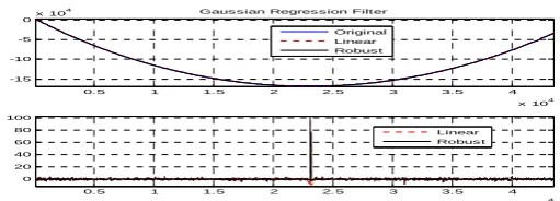
of comparing speed and accuracy. Figure 1 is a simulated profile (43000 pts) with

significant form component and a noticeable pip in the middle of the profile. Figure 2

outlier spikes. The convolution algorithms need several hours to get the results, while

the fast algorithms proposed only need several hundred milliseconds in all cases.

0.5 1 1.5 2 2.5 3 3.5 4

x 104

-15 -10 -5

0x 10

4 Gaus sian Regress ion Filter

Original Linear Robust

0.5 1 1.5 2 2.5 3 3.5 4

x 104

0 20 40 60 80 100

Linear Robus t

Figure 1: simulated data (up: original and mean profile; down: residual profile)

2000 4000 6000 8000 10000 12000 14000 16000 18000

-1400 -1200 -1000 -800

Gaus sian Regres s ion Filter

Original Linear Robust

2000 4000 6000 8000 10000 12000 14000 16000 18000

-300 -200 -100 0

Linear Robust

Figure 2: measured profile (up: original and mean profile; down: residual profile)

5 Conclusions

In this paper, the authors have reviewed the linear and nonlinear Gaussian regression

filters of zeroth, second order. Fast algorithms based on the FFT method have also

been proposed. Experiments have shown that the new algorithms have improved the

speed significantly and achieved similar compatible accuracy.

6 Acknowledgement

The authors would like to thank the EPSRC in the UK for support fund to carry out

this research work under its programme EP/F032242/1.

References:

[1] ISO 11562 1996 Geometrical Product Specification (GPS) – Surface texture:

Profile method – Metrological characteristics of phase correct filters

[2] Brinkmann S, Bodschwinna H 2001 Accessing roughness in three-dimensions

using Gaussian regression filter, Int. J. of Mach. Tools & Manuf. 41 2153-2161

[3] Seewig J 2005 Linear and robust Gaussian regression filters, Journal of Physics: