Non-perturbative Massive de Sitter Solutions
Zurab Kakushadze
1QuantigicrSolutions LLC, 1127 High Ridge Road #135, Stamford, CT 06905∗
2Department of Physics, University of Connecticut, 1 University Place, Stamford, CT 06901
∗Corresponding Author: [email protected]
Copyright c⃝2014 Horizon Research Publishing All rights reserved.
Abstract
We discuss non-perturbative dynamics of massive gravity in de Sitter space via gravitational Higgs mechanism. We argue that enhanced local symmetry and null (ghost) state at (below) the perturbative Higuchi bound are mere artifacts of not only linearization but also assuming the Fierz-Pauli mass term. We point out that, besides de Sitter, there are vacuum solutions where the space asymptotically is de Sitter both in the past and in the future, the space first contracts, this con-traction slows down, and then reverses into expansion, so there is an epoch where the space appears to be (nearly) flat, even though the vacuum energy density is non-vanishing. We confirm this by constructing a closed-form exact solution to full non-perturbative equations of motion for a “special” massive de Sitter case. We give a formula for the “critical” mass above which such solutions apparently do not exist. For the Fierz-Pauli mass term this “critical” mass coincides with the perturbative Higuchi bound, and the former serves as the non-perturbative reinterpretation of the latter. We argue that, notwithstanding the perturbative ghost, non-perturbatively there is no “instability”. Instead, there are additional vacuum solutions that may have interesting cosmological implications, which we briefly speculate on.Keywords
Massive Gravity, Gravitational Higgs Mechanism, de Sitter Space, Non-perturbative Solutions, Contraction and Expansion1
Introduction and Summary
The currently observed accelerated expansion of the Universe [1, 2] is one of the motivations for considering large-scale modifications of gravity. One such modification is giving small mass to the graviton with the aim of explaining the accelerated expansion without a tiny cosmological constant.1 While – barring unbroken supersymmetry – the cosmological constant is
not protected, quantum corrections to the graviton mass appear to be suppressed by the graviton mass itself [3]. However, unlike in a scalar or vector theory, in gravity there is more to the graviton mass.
A general Lorentz invariant mass term for the gravitonhM N in the linearized approximation is of the form
−M2
4
[
hM NhM N−β(hMM)
2] ,
(1) whereβ is a dimensionless parameter. Perturbatively,2forβ ̸= 1the trace componenthM
M is a propagating ghost, while it decouples in the Minkowski background for the Fierz-Pauli mass term withβ = 1[4]. Again, perturbatively, generically a ghost reappears beyond the linearized level even for the Fierz-Pauli mass term [5] and, once again, perturbatively, to avoid the reappearance of a ghost beyond the linearized level one attempts tuning the mass term to a special form [3]. On the other hand, while quantum mechanically small graviton massM per semay well be “technically natural” [3], the special form of the mass term necessary for avoiding a ghost beyond the linearized level is not protected by any symmetry. In fact, already at the linearized levelβin (1) is not protected by any symmetry against quantum corrections. Does this then mean that massive gravity is “unstable”?
Gravitational Higgs mechanism [6, 7] provides a non-perturbative and fully covariant definition of massive gravity. Non-perturbatively, even forβ ̸= 1, the Hamiltonian is bounded from below and the perturbative ghost is merely an artifact of
∗DISCLAIMER: This address is used by the corresponding author for no purpose other than to indicate his professional affiliation as is customary in
scientific publications. In particular, the contents of this paper are limited to Theoretical Physics, have no commercial or other such value, are not intended as an investment, legal, tax or any other such advice, and in no way represent views of QuantigicrSolutions LLC, the website www.quantigic.com or any of their other affiliates.
1 Notwithstanding that zero cosmological constant might be just as “unnatural”. 2 Here we refer to perturbative expansion in powers ofh
linearization [8, 9].3 Therefore, stability should be addressed in the context of full non-perturbative theory. Furthermore,
since there is no symmetry that would protectβ, there appears to be no reason to restrict toβ = 1. In particular, if there is any “instability”, it should be visible non-perturbatively. For instance, in [11], in furtherance of the results of [9], explicit non-perturbative vacuum massive solutions were constructed in the case of gravitational Higgs mechanism in Minkowski space.4 There appears to be no “instability” or catastrophic collapse of the background. Instead, non-perturbatively there simply exist vacuum solutions other than the Minkowski background. These vacuum solutions are oscillatory with no evident pathologies or cause for alarm. That is, despite the fact that perturbatively there is a fake ghost, non-perturbatively the theory does not appear to be “sick” or inconsistent. In fact, it has a rich structure of apparently well-behaved (non-static) vacuum solutions.5
Motivated by these results and also by the observation of [12], in this note we discuss non-perturbative dynamics of massive gravity in de Sitter space via gravitational Higgs mechanism. We keepβarbitrary. Forβ = 1, perturbatively there is the Higuchi bound [13], according to which the helicity-0 graviton mode becomes null atM2 = 2H2 and turns into a
ghost forM2<2H2(whereHis the Hubble parameter in de Sitter space), which is a form of vDVZ discontinuity [14, 15].
The appearance of the null state atM2 = 2H2is due to enhanced local symmetry [16, 13, 17]. However, as was argued in
[8], non-perturbatively there is no enhanced symmetry or null state for any value of the graviton mass and these are merely artifacts of linearization as is the perturbative ghost. In this paper we first consider the linearized theory for generalβ and argue that forβ ̸= 1there is no enhanced symmetry or null state already at the linearized level. So, in this regard, these are artifacts of not only linearization but also assuming the Fierz-Pauli mass term.
We then discuss full non-perturbative equations of motion for generalβandM2/H2. For generalβand dimensionDthe analog of the perturbative Higuchi bound is
M∗2=(D−1)(D−2)
Dβ−1 H
2
. (2)
However, we emphasize that non-perturbatively there is no enhanced local symmetry or null state atM2=M2
∗, and there is
no ghost atM2 < M2
∗. Instead, the significance of the “special point”M2 =M∗2is that it delineates the types of vacuum
solutions other than de Sitter that exist. Thus, we argue that there exist vacuum solutions which asymptotically are de Sitter for bothτe→ ±∞, whereeτis the “proper time”, and have the property that the space (starting from de Sitter ateτ→ −∞) first contracts, this contraction slows down, and then reverses into expansion (ending with de Sitter ateτ →+∞), so there is an epoch where the space appears to be (nearly) flat, even though the vacuum energy density is non-vanishing.6 Such solutions
exist for allM2≤Mc2, whereMcis the “critical” graviton mass. It is convenient to parameterizeM2via1−α≡M∗2/M2, soα∈(−∞,1), andα= 0corresponds toM2=M∗2. We derive an exact formula for the valueαc corresponding toMc2 for arbitraryβandD(see Section 5, Eq. (59) for details):
αc ≡
D−1
D+3+1−ββ , (3)
so the aforementioned vacuum solutions do not exist forα > αc, or forM2> Mc2, where
Mc2= M
2 ∗
1−αc
= (D−1)(D−2)
4(Dβ−1) (D(1−β) + 3 +β)H
2. (4)
Forβ= 1(the Fierz-Pauli case) we haveM2
c = (D−2)H2=M∗2, so there are no such asymptotic solutions forM2> M∗2 in this case, while forM2 ≤ M2
∗ we do have such solutions. And non-perturbatively this is the meaning of the Higuchi
bound forβ = 1. Forβ ̸= 1it isM2
c, notM∗2, that carries this meaning, albeitM∗2defined in (2) does serve as a more subtle “demarkation line” for more detailed properties of these vacuum solutions (see Section 4 for details).
In fact, forβ = 1/2andα= 0(i.e., at the “special point”M2 =M2
∗) we solve the full non-perturbative equations of
motion in closed form and explicitly construct the solution described above (see Eq. (39) and the subsequent discussion for details). (We have also constructed it numerically as an additional check, see Fig.1.) Just as in the Minkowski case [11], we find no “instability” or catastrophic collapse of the background. Instead, non-perturbatively there simply exist vacuum solutions other than de Sitter. An interesting feature of these solutions is the initial contraction and the subsequent expansion, with an epoch where the space-time appears to be (nearly) flat. And this is irrespective of the value of the cosmological constant. Such solutions may be interesting in the context of the cosmological constant problem.E.g., one could imagine that we live in such a universe and the “observed value” of the cosmological constant (i.e., the accelerated rate of expansion) is small because we are just past the turning point and starting to expand. Another possible application could be in the context of inflation and the Big Bang. In particular, one could imagine a scenario where the space contracts to a small (Planckian) size and then expands again, providing the “starting point” for the Universe. Just speculations. . .
To summarize, despite the fact that perturbatively there is a fake ghost, non-perturbatively the theory does not appear to be “sick” or inconsistent. In fact, it has a rich structure of (possibly interesting) vacuum solutions. The remainder of this 3 The full non-perturbative Hamiltonian for the model of [7], which hasβ= 1/2, in the gravitational Higgs mechanism framework was constructed in [10] and is expressly positive-definite. Non-perturbative unitarity for generalβin the Minkowski space was argued in [9], while for the de Sitter space it was argued in [8]. For a list of other works related to gravitational Higgs mechanism and massive gravity, see [11] and [3].
4 That is, Minkowski space being one of the background solutions.
5 Whether there are any tunneling effects is a separate and interesting topic for investigation.
note is organized as follows. In Section 2 we very briefly review gravitational Higgs mechanism in curved backgrounds. In Section 3 we discuss linearized massive gravity in de Sitter space. In Section 4 we discuss non-perturbative dynamics in the
β = 1/2case and give the explicit exact solution forα= 0. In Section 5 we derive the formulas forαcandMc2for general
β.
2
Gravitational Higgs Mechanism
In this section we very briefly review gravitational Higgs mechanism in curved backgrounds – de Sitter was discussed in [8], and the general case in [11]. We start with gravity inDdimensions
SG≡MPD−2
∫
dDx√−G
[
R−Λe
]
, (5)
whereΛe is the cosmological constant. LetGeM N be a background solution to the equations of motion corresponding to (5). The background metricGeM Ngenerally is a function of the coordinatesxS:GeM N =GeM N(x0, . . . , xD−1).
Let us now introduceDscalarsϕA. Let us normalize them such that they have dimension of length. Let us define a metric
ZABfor the scalars as follows:
ZAB(ϕ0, . . . , ϕD−1)≡δAMδBNGeM N(ϕ0, . . . , ϕD−1). (6) Next, consider the induced metric for the scalar sector:
YM N =ZAB∇MϕA∇NϕB. (7)
The following action, albeit not most general,7will suffice for our purposes here:
SY =MPD−2
∫
dDx√−G[R−µ2V(Y)] , (8)
wherea priorithe “potential”V(Y)is a generic function ofY ≡YM NGM N, andµis a mass parameter, whileΛeis subsumed in the definition ofV(Y).
The equations of motion have the following solutions
ϕA=δAM xM , (9)
GM N =GeM N, (10)
with
e
Λ =µ2[V(D)−2V′(D)] . (11)
The scalar vacuum expectation values break diffeomorphism spontaneously, and the equations of motion are invariant under the full diffeomorphism invariance. We can therefore set the scalars to their background values, which leaves us with pure gravity:
SM G=MPD−2
∫
dDx√−G[R−µ2V(X)] , (12) whereX ≡GM NGe
M N. The equations of motion read
RM N =µ2
[
V′(X)GeM N+
V(X)−X V′(X)
D−2 GM N
]
, (13)
with the Bianchi identity
∂M
[√
−GV′(X)GM NGeN S
]
−1
2
√
−GV′(X)GM N∂SGeM N = 0, (14) which is equivalent to the gauge-fixed equations of motion for the scalars.
In the linearized approximation in (13) we have the mass term corresponding to (1) with
M2≡2µ2V′(D), (15)
β ≡1
2 −
V′′(D)
V′(D) . (16)
We haveβ = 1for potentialsV withV′(D) =−2V′′(D). For a linear potentialV(X) =a+X, we have the model of [7] withβ= 1/2(and fora=−(D−2)we have the Minkowski background).E.g., for quadratic potentialsV =a+X+λX2
withλ̸= 0we can have other values ofβ, includingβ= 1forλ=−1/2(D+ 2). 7One can consider a more general setup with the scalar action constructed not just fromY, but fromY
3
Massive Gravity in de Sitter
In this section we study linearized equations of motion for the de Sitter background metricGeM N ≡(Ht)−2ηM N, where
t≡x0,His the constant Hubble parameter,H2≡Λe/(D−1)(D−2), andηM N is the Minkowski metric. Let us keepβin (16) arbitrary for now. LetGM N ≡GeM N+hM N andh≡GeM NhM N. Then the linearized equations of motion (13) read:
SM N = 0, (17)
SM N ≡hM N+∇M∇Nh−2∇(M∇ShN)S−GeM N
[
h− ∇S∇RhSR
]
−
H2
[
2hM N + (D−3)GeM Nh
]
−M2
[
hM N−βGeM Nh
]
, (18)
where∇M is the covariant derivative in the de Sitter background metricGeM N, and≡GeM N∇M∇N. Furthermore, the Bianchi identity (14) reduces to
∇Nh
M N−β∇Mh= 0. (19)
Note that (19) follows from (17).
3.1
Enhanced Local Symmetry at
β
= 1
For the Fierz-Pauli mass terms (β = 1) at a special value of the ratioΛe2/M2the linearized equations of motion (17) are
invariant under the following infinitesimal local transformations:
δhM N = (∇M∇N+H2GeM N)χ . (20) This local symmetry is present when
M2= (D−2)H2. (21)
The following identities are useful in deriving this result:
(∇M − ∇M )χ= (D−1)H2∇Mχ , (22)
(∇M∇N − ∇M∇N )χ= 2H2
(
D∇M∇N −GeM N
)
χ . (23)
InD= 4the presence of the symmetry (20) at the point (21) was discussed in [16].
The presence of this additional local symmetry in the linearized theory implies that at the point (21) the graviton has (D+ 1)(D−2)/2−1propagating degrees of freedom (as the helicity-0 graviton mode has null norm), one fewer than at generic points in the parameter space. Furthermore, the linearized theory is non-unitary forM2<(D−2)H2(as the
helicity-0 graviton mode has negative norm), while forM2>(D−2)H2all(D+ 1)(D−2)/2graviton modes are propagating and
have positive norm [16, 13, 17]. Also, in the linearized theory atM2 = (D−2)H2 the gravitonh
M N can only couple to traceless conserved energy-momentum tensorTM Nas the coupling to the trace part ofTM Nis inconsistent with the symmetry (20). For a recent discussion, see [18, 19].
However, as was argued in [8], the appearance of the enhanced local symmetry at M2 = (D−2)H2is an artifact of
linearization. There is no enhanced local symmetry in the full nonlinear theory, nor is there a null state or a ghost, and the full nonlinear theory unitary is for all values ofM2/H2with no vDVZ discontinuity. The purpose of our exercise here is to
argue that the enhanced local symmetry (and all its consequences) is not only an artifact of linearization but also of requiring the Fierz-Pauli term. This is reminiscent to what transpires in static radially symmetric solutions withΛ = 0e – as was argued in [12], there is no vDVZ discontinuity in the perturbative asymptotic solutions except forβ = 1.
3.2
General
β
It is not difficult to see that the symmetry
δhM N = (∇M∇N +γH2GeM N)χ , (24) whereγis an arbitrary dimensionless constant, is not a symmetry of the linearized equations of motion forβ ̸= 1. Indeed, (19) is not invariant under these transformations unlessβ = 1. It then follows that there cannot be any null state forβ ̸= 1. Without a null state we do not expect a transition between the regime without a ghost to a regime with a ghost either. I.e., what transpires atM2= (D−2)H2in theβ= 1case is an artifact ofβ= 1and does not happen at other values ofβ.
We can see this explicitly by studying the linearized equations of motion. The simplest way to proceed is to focus on the relevant graviton degrees of freedom, namely, the conformal modeωand the helicity-0 modeρ. These two modes are related via (19). LethM N =GeM Nω+∇M∇Nρ. Then (19) gives
(Dβ−1)ω= (D−1)H2ρ+ (1−β)ρ . (25)
To see this more explicitly, let us look at the full equations of motion. The equation of motion for the tracehreads:
−(D−2)(1−β)h+[(Dβ−1)M2−(D−1)(D−2)H2]h= 0. (26) Again, for β = 1 this equation is algebraic and generally implies that h = 0. At the special point with β = 1 and
M2 = (D−2)H2, this equation reduces to an identity, which is a manifestation of the enhanced local symmetry at this
point. Furthermore, if we included a matter source, the r.h.s. of (26) would be proportional to the trace of the conserved energy-momentum tensor, which therefore must vanish forβ = 1andM2= (D−2)H2. However, forβ ̸= 1nothing of the
kind transpires as thehterm is present regardless of the value ofM2/H2.
Let us take this a step further and analyzeSM N in (18) for the modesωandρ. A little algebra gives
SM N = (D−2)
[
∇M∇N ω−GeM Nω
]
−(D−1)(D−2)H2GeM N ω , (27) where we have used (22) and (25), and
ω≡ω− M
2
D−2 ρ=
[
D−1
Dβ−1 H
2− M2
D−2
]
ρ+ 1−β
Dβ−1 ρ . (28)
Note that whenβ= 1, we haveω=[H2−M2/(D−2)]ρ, soρis null atM2= (D−2)H2, is a ghost atM2<(D−2)H2, and is a positive-norm state forM2 >(D−2)H2. However, forβ ̸= 1there is no null state. Instead, we have a higher-derivative equation of motion for ρ. We will not analyze this linearized higher-derivative equation of motion from the viewpoint of stability – as was argued in [8], stability needs to be addressed non-perturbatively (and was discussed in detail in [8]) as the linearization artificially introduces a ghost,8including forβ ̸= 1. And we will discuss non-perturbative solutions momentarily. Our key observation here is that the enhanced local symmetry at the special point and its consequences are merely an artifact of requiring the Fierz-Pauli mass term.
4
Non-perturbative Dynamics
Looking at (26) or (28), one might get an uneasy feeling that even forβ ̸= 1something funny might transpire as the graviton mass crosses the “special point” defined as
M2=M∗2≡ (D−1)(D−2)H
2
Dβ−1 =
e
Λ
Dβ−1 . (29)
E.g., one may even worry about a potential tachyonic instability. As mentioned above, stability must be analyzed non-perturbatively, which was done in [8] by studying the non-perturbative Hamiltonian, which was argued to be bounded from below, hence no ghost or instability. Here we will not repeat the analysis of [8], but instead complement it by studying solutions to full non-perturbative equations of motion, similarly to the Minkowski case in [11].
The equations of motion (13) are highly nonlinear. However, we can get a handle on them by considering linear potential
V =a+X[7]. In this case we haveΛ = (e a+D−2)µ2,M2= 2µ2,β= 1/2andM2
∗/M2= 1−α, whereα≡ −a/(D−2),
so the “special point” corresponds toα= 0. The equations of motion (13) read
RM N =µ2
[ e
GM N −αGM N
]
. (30)
The naively “troublesome” case is whenαis negative.
4.1
“Special Point”:
α
= 0
(for
β
= 1
/
2
)
Let us start with studying non-perturbative solutions at the “special point”α= 0. We will look for the solutions of the form
GM N =diag(exp(2B)η00,exp(2A)ηii). (31)
Then we haveRi0= 0and (prime denotes derivative w.r.t.t):
R00=−(D−1)
[
A′′−A′B′+ (A′)2
]
, (32)
Rij =
[
A′′−A′B′+ (D−1) (A′)2
]
exp(2A−2B)δij, (33)
and the(00)and the(ij)equations of motion read:
A′′−A′B′+ (A′)2=t−2, (34)
A′′−A′B′+ (D−1) (A′)2= (D−1) exp(2B−2A)t−2, (35) 8 In fact, as was argued in [9], the intrinsically perturbative parametrizationh
where we have taken into account that atα= 0we haveµ2= (D−1)H2. The Bianchi identity (14) reduces to
t−1[(D−1) exp(2B−2A)−1] + (D−1)A′−B′ = 0, (36) which together with the equations of motions allows to eliminateB′:
B′ = (D−2)t(A′)2+ (D−1)A′. (37) The(00)equation then reduces to the following first-order nonlinear equation:
Qτ= [1 +Q]
[
1 + (D−2)Q2] , (38)
whereQ ≡ tA′ = Aτ ≡ ∂τA, andQτ ≡ ∂τQ, where∂τ ≡ t∂t. Note that the background solution GM N = GeM N corresponds to theQ=−1solution of (38). However, we have another vacuum solution given by
ln|1 +Q| − 1
2ln
(
(D−2)−1+Q2)+√D−2 tan−1
(√
D−2Q
)
=
(D−1) (τ−τ0) , (39)
whereτ0is an integration constant. In fact, there are two inequivalent solutions, which we will refer to asQ(±), with the
following properties. TheQ(±) solutions are defined for τ ∈ (−∞, τ(±)
∗ ), whereτ∗(±) ≡ τ0(±)±
√
D−2π/2(D−1), and we haveQ(+) > −1, Q(−) < −1, atτ → −∞ we haveQ(±) → −1±, Q(+) monotonically increases from −1
to+∞, and Q(−) monotonically deceases from −1 to−∞. As we will see in a moment, the singularities at τ∗(±) are not true singularities but mere coordinate singularities with finite “proper time”. To obtain a geodesically complete space, we must continue each solution through this coordinate singularity. To do this, let us study the behavior of the metric at
τ → τ∗(±)−. We have(Q(±))2 ∼ 1/2(D−2)(τ(±)
∗ −τ)andQ(±) ∼ ±1/
√
2(D−2)(τ∗(±)−τ), which implies that
A(±)∼A(∗±)∓
√
2(τ∗(±)−τ)/(D−2), whereA∗(±)are constants, soA(±)are finite atτ→τ∗(±)−, albeit their derivatives w.r.t. τare not. Furthermore, we haveB(±)∼ −ln(τ(±)
∗ −τ
)
/2, soB(±)are singular. However, this is just a coordinate
singularity due to the choice of the time coordinateτ. The Ricci tensor is finite and so is the scalar curvature.9 Furthermore,
this coordinate singularity is at finite “proper time”. Thus, first note thatτ = ln(ν(±)t), whereν(±)are integration constants
for the Q(±) solutions. Let t(±)
∗ correspond toτ∗(±): t(∗±) ≡ exp(τ∗(±))/ν(±). Let us further define the “proper time”
deτ ≡ exp(B(±))dt. Since,dt = tdτ, asτ → τ(±)
∗ −, we havedeτ ∼ t(∗±)exp(B(±))dτ ∼ t(∗±)dτ /
√
τ∗(±)−τ, and
e
τ ∼τe∗(±)−2t(∗±)
√
τ∗(±)−τ, where eτ∗(±)are constants corresponding toτ∗(±),i.e., these values of the “proper time” are finite. Also, note thatA(eτ±)∼ ±1/√2(D−2)t(∗±), so the derivative ofAw.r.t. the “proper time” is finite. Furthermore, note that atτ → −∞we haveB(±) → −τ, anddeτ ∼dτ /ν(±), so even thoughτ → −∞, we can haveeτ →+∞oreτ → −∞
depending on the sign ofν(±).
The metric in the “proper time” (or flat slicing) coordinates is given by
ds2∼ −deτ2+ exp(2A)δijdxidxj, (40)
which is finite. Now we can sew theQ(±)solutions together to obtain a geodesically complete space. Thus, consider the
following solution. LetA(+)∗ =A(∗−)≡ A∗. t(+)∗ =−t∗(−) ≡t∗,ν(+) =−ν(−) ≡ν,τ(+)
∗ =τ∗(−) ≡τ∗(which implies
thatτ0≡τ (+) 0 =τ
(−) 0 −
√
D−2π/(D−1)). Furthermore, letτe∗(+)=eτ∗(−)≡eτ∗. Then we have a smooth solution defined foreτ ∈Rsuch thatQ≡Aτ is given byQ =Q(±)foreτ ∈R∓eτ whenν >0, andQ=Q
(±)foreτ ∈R± e
τ whenν <0, whereR−x ≡(−∞, x]andR+x ≡[x,+∞). Note thatAis continuous andAeτ is also continuous (even thoughAτ is not). Theν >0andν <0solutions are mirror to each other undereτ→ −eτ. For definiteness, without loss of generality, we will therefore assumeν >0.
In this solution atτe→ −∞we have de Sitter space. Aseτincreases, the space contracts, but this contraction slows down and stops atτe=eτ1, whereeτ1corresponds toτ1 ≡τ0+ ln(D−2)/2(D−1) < τ∗ ≡τ0+
√
D−2π/2(D−1), and for
e
τ >τe1the space starts to expand, seamlessly goes through the “sewing” pointeτ=eτ∗and continues to expand asymptotically
approaching de Sitter ateτ →+∞. The interesting feature of this solution is that there is an epoch where the space appears to be (nearly) flat, which is neareτ =eτ1. And this occurs regardless of the value of the cosmological constantΛ. In fact, thise
solution is a “no-scale” solution despite the fact that there is a mass scale in the theory. In particular, if we rescaleν →λν, whereλis a constant, the solution is the same as before with the rescalingτe→eτ /λ. Fig.1 shows this solution withD = 4,
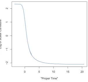
ν = 1,τe1= 0andA(eτ1) = 0. Fig.2 showsln(R/µ2). Even though there is no small parameter, the scalar curvatureRdrops
about two orders of magnitude fromR(τe→ −∞)≈10.2µ2toR(τe→+∞)≈0.123µ2.
9 Before fixing the gauge by setting the scalars to their background values via (9), we have additional gauge invariantsGM N∂
MϕA∂NϕB, which upon
gauge fixing reduce toGM N. SinceAis finite andBgoes to+∞atτ→τ(±)
−5 0 5 10 15 20 25 30
0
1
2
3
4
"Proper Time"
L
o
g
a
ri
th
mi
c
Sca
le
F
a
ct
o
[image:7.595.126.435.104.386.2]r
Figure 1. Exact solution (D= 4,ν = 1) of Subsection 4.1. x-axis: “proper time”τ;e y-axis:Ain (40). (We have seteτ1andA(τ1e)to 0 in (40) – see Subsection 4.1.)
0 5 10 15 20
−2
−1
0
1
2
"Proper Time"
L
o
g
o
f
Sca
la
r
C
u
rv
a
tu
re
[image:7.595.131.436.491.775.2]4.2
General
α
(for
β
= 1
/
2
)
In the case of generalα, whereα∈(−∞,1), the above equations of motion forQandBare more complicated:
Qτ =
(D−1)(Q+ 1) (1−α)(D−2) +
[
Q− 1
(1−α)(D−2)
] e
Bτ, (41)
e
Bτ= (1−α)(D−2)Q2+ (D−1)Q+α(D−2)e2Be+ 1, (42) whereBe ≡B+ ln(Ht). It will also be useful to rewrite (41) and (42) as follows:
Qτ = (Q+ 1)
[
(1−α)(D−2)Q2+α(D−2)Q+ 1]+
α(D−2)
[
Q− 1
(1−α)(D−2)
] [
e2Be−1
]
. (43)
e
Bτ = (Q+ 1) [(1−α)(D−2)Q+α(D−2) + 1] +
α(D−2)
[
e2Be−1
]
. (44)
So we have a system of two first order nonlinear differential equations, which is difficult to solve in closed form for general
α. (Note that forα= 0the exponential term vanishes and the system reduces to a first order nonlinear differential equation forQ, which we solved above.) Happily, we do not need to solve this system in closed form to understand if there is a ghost or tachyonic instability forα <0(orα >0for that matter).
First, note that irrespective of the value ofαwe have the de Sitter solution whereQ ≡ −1andBe ≡ 0. The question is whether there are any other solutions as in theα = 0case. Asymptotically, at |τ| → ∞,a prioriwe can have Q →
const. or|Q| → ∞. Let us show that asymptotically we cannot have |Q| → ∞. From (41) we have Be ∼ ln|Q| −
(D−1)(τ −τ0)/(1−α)(D−2)in this case, whereτ0 is an integration constant. Then (42) implies thatQτ ≈ (D − 2)Q3[1−α+αexp (−2(D−1)(τ−τ
0)/(1−α)(D−2))]. This, in turn, implies that |Q| → ∞ must occur at finite
τ → τ∗. Indeed, let us first assume that|Q| → ∞occurs atτ → +∞. Then we would haveQτ ≈(1−α)(D−2)Q3, whose solution behaves as1/Q2 ∼ 2(1−α)(D −2)(τ∗−τ), where τ∗ is an integration constant, so our assumption that |Q| → ∞occurs at τ → +∞ does not hold. Next, let us assume that|Q| → ∞ occurs atτ → −∞. Then we would have Qτ ≈ (D −2)αQ3exp (−2(D−1)(τ−τ0)/(1−α)(D−2)), whose solution behaves as1/Q2 ∼ α(1−
α)(D−2)2exp (−2(D−1)(τ−τ0)/(1−α)(D−2))/(D−1), so our assumption that|Q| → ∞occurs atτ → −∞
also cannot be correct. Since|Q| → ∞can only occur at finiteτ → τ∗, we have1/Q2 ∼ 2(D −2)ζ(τ
∗−τ), where
ζ ≡1−α+αexp (−2(D−1)(τ∗−τ0)/(1−α)(D−2)). Whether|Q| → ∞occurs atτ →τ∗+orτ →τ∗−depends
on the sign ofζ: forζ > 0it occurs atτ →τ∗−, while forζ <0it would occur atτ →τ∗+. Sinceα <1, forα≥0we haveζ >0. Forα <0we need to dig deeper (see below). In any event, just as forα= 0, there is a coordinate singularity at
τ =τ∗, the space is geodesically incomplete, and in any physically meaningful solution we would have to continue through theτ=τ∗point by sewing two geodesically incomplete solutions withQgoing to the opposite infinities asτ→τ∗from two different sides ofτ∗, just as in theα= 0case.
Now that we have established that asymptotically we can only haveQ→const., asymptotically we have three possibili-ties:i)Be→const.,ii)Be→+∞, andiii)Be → −∞. Let us assume that asymptotically we haveBe→const., soBeτ →0. SinceQeτ →0, (41) implies that we must haveQ→ −1, and then (44) implies thatBe→0. We can therefore linearize (43) and (44) in the asymptotic regime:Q=−1 +q, where|q| ≪1and|Be| ≪1:
qτ≈[(1−2α)(D−2) + 1]q− 2α
1−α[(1−α)(D−2) + 1]B ,e (45)
e
Bτ ≈ −[(1−2α)(D−2)−1]q+ 2α(D−2)B .e (46) So, we have a system of first order linear differential equations with constant coefficients. Then we haveq∼q1exp(λτ)and
e
B ∼Be1exp(λτ), whereλcan take two values given by the eigenvaluesλ1andλ2of the2×2matrixDof the coefficients
in the system (45) plus (46). Fromλ1+λ2=Tr(D) = (D−1)andλ1λ2= det(D) = 2α(D−1)/(1−α)we get
λ1,2=
D−1 2
[
1±
√
1−α/αc 1−α
]
, (47)
where
αc≡
D−1
D+ 7. (48)
That is, forα > αcsuch asymptotic solutions do not exist. This occurs when graviton mass isM2> Mc2, where
Mc2≡ M
2 ∗
1−αc = 1
4(D−1)(D+ 7)H
2. (49)
Forα=αcthe eigenvalues are degenerate. For0< α < αcboth eigenvalues are positive, so such asymptotic solutions can only occur atτ→ −∞, which is consistent with what we found above that forα >0, where we can only have|Q| → ∞
atτ→τ∗−. Forα= 0one of the eigenvalues vanishes:λ2= 0; this is, as we found above, because in this case we have a
first order differential equation forQ. Whenα <0,λ1is positive, whileλ2is negative. So, we can have two different types
of solutions, one whereQ→ −1atτ → −∞and|Q| → ∞atτ →τ∗−, and the other whereQ→ −1atτ →+∞and
|Q| → ∞atτ →τ∗+. As we mentioned above, we must sew two geodesically incomplete solutions atτ =τ∗to obtain a geodesically complete solution, which, as in theα= 0, case asymptotically goes to de Sitter (Q→ −1) on both ends.
We still need to check if we can haveBe →+∞or−∞asymptotically. In the former case from (42) we haveBeτ ∼α(D− 2) exp(2Be), whose solution behaves asexp(−2Be)∼ −2ατ, so our assumption thatBe→+∞does not hold. However,a pri-oriwe could haveBe→ −∞. In this case from (41) and (42) it follows thatQτ∼[Q+ 1/(1−α)]
[
(1−α)(D−2)Q2+ 1],
so we invariably haveQ→ −1/(1−α)andBeτ → −α/(1−α). Furthermore, forα >0this can only occur atτ → −∞. This is because in this case asymptotically we must haveq→0, whereq≡Q+1/(1−α), and we haveqτ ≈(D−1+α)/(1−α)q, and the coefficient in front ofqis positive forα > 0. However, since the assumption is thatBe → −∞, this implies that forα >0 this could only occur asτ → +∞as we haveBeτ → −α/(1−α). So, such asymptotic solutions cannot exist forα > 0. On the other hand, forα < 0 we can haveBe → −∞only at τ → −∞, which implies that we must have
α >−(D−1). Furthermore, we haveB =Be−τ∼ −τ /(1−α), soB →+∞. Also,A∼ −τ /(1−α)→+∞. For the scalar curvature we have
R=µ2
[
GM NGeM N−D
]
=
µ2
[
1
H2t2
(
e−2B+ (D−1)e−2A)−D
]
∼Dν2µ2exp
(
2ατ
1−α
)
→+∞, (50)
whereν is an integration constant (fromt= exp(τ)/ν). So, we have a singularity. In fact, this is a naked singularity. Thus, for the “proper time” we havedeτ ≡ exp(B)dt = exp(B+τ)dτ /ν = exp(Be)dτ /ν, so we haveeτ → eτ0 as τ → −∞,
whereeτ0is a finite integration constant. That is, we have a true naked singularity at a finite “proper time”. So,Be → −∞
solutions are not physical and must be discarded.10 Forα < 0this leaves us with solutions where asymptoticallyQ→ −1
andBe →0. Note that the only solution where asymptotically we haveQ → −1for bothτ → −∞andτ → +∞is the de Sitter solution itself whereQ≡ −1. In all other solutions asymptotically we haveQ → −1 atτ → −∞or+∞and
|Q| → ∞atτ → τ∗−respectivelyτ → τ∗+, and atτ = τ∗ we must sew two geodesically incomplete solutions into a geodesically complete solution as in theα= 0case.11
5
α
cfor General
β
Let us study the full equations of motion (13) and (14) with the metric of the form (31). Our goal in this section is to deriveαc for generalβ. To do this, let us assume that the metricGM N asymptotically approaches the background metric
e
GM N, so we haveA≡ −ln(Ht) +Ae,B ≡ −ln(Ht) +Be, and eventually we will keep only the linear terms inAeandBe. The exact equations of motion read:
e
Λ
µ2
[ e
Aτ τ +Beτ−AeτBeτ
]
=−V′(X)(D−1)
[
e2Be−2Ae−1
] , (51) e Λ µ2 ( e
Aτ−1
)2
=V′(X)
[
(D−1)e2Be−2Ae−1
]
+ [V(X)−XV′(X)]e2Be, (52) (D−1)
[
e2Be−2Ae−1
]
+ (D−1)Aeτ−Beτ+
V′′(X)
V′(X) Xτ = 0. (53) The linearized expression forXis given byX =D−2
[
(D−1)Ae+Be
]
, so we have
(D−1)A= (D−1)
[
βq+Be
]
−(1−β)Beτ, (54)
X=D−2
[
DBe+ (D−1)βq−(1−β)Beτ
]
, (55)
whereq ≡ Aeτ,M∗2/M2 ≡ 1−α,M2 = 2µV′(D),M∗2 = Λe/(Dβ−1),Λ = (e D−1)(D−2)H2, andβ ≡ 1/2−
V′′(D)/V′(D). So, we have the following system:
qτ =
[
(D−1)−α(Dβ−1)
β(1−β)
]
q− α
1−α
[
D−1 1−β −
α(Dβ−1)
β(1−β)
] e
B , (56)
e
Bτ =−
[
(D−1)− 1
β −
α(Dβ−1)
β(1−β)
]
q+α(Dβ−1)
β(1−β) B .e (57)
10Perhaps adding higher-curvature terms could smooth out this singularity.
Let the matrix of the coefficients on the r.h.s. beD. Then the eigenvalues of this matrixλ1 andλ2 satisfy the following
equations:λ1+λ2=Tr(D) = (D−1), andλ1λ2= det(D) =α(D−1)/(1−α)(1−β). This implies that
λ1,2=
D−1 2
[
1±
√
1−α/αc 1−α
]
, (58)
where
αc ≡
D−1
D+3+1−ββ , (59)
so solutions (other than de Sitter itself) where asymptotically we have de Sitter do not exist forα > αc, or forM2 > Mc2, where
Mc2=
M∗2
1−αc
= (D−1)(D−2)
4(Dβ−1) (D(1−β) + 3 +β)H
2. (60)
Note that forβ = 1we haveM2
c = (D−2)H2 =M∗2, so there are no such asymptotic solutions forM2 > M∗2in this case, while forM2 ≤ M2
∗ we do have such solutions. This is the restatement of the Higuchi bound forβ = 1: the naive
perturbative ghost instability forM2< M2
∗ translates into the fact that we have other solutions to the full non-perturbative
equations of motion where the space is de Sitter only asymptotically. There is nothing “wrong” with these solutions, in fact, perhaps they are even more interesting than de Sitter. But there is no catastrophic “instability” such as the space-time collapsing; there is a contraction followed by an expansion with an epoch where the space appears to be (nearly) flat. Also, note that forβ = 1/Dwe haveαc= 1/(D−1), albeitM∗is infinite at this point, and so isMc, so we have such asymptotic solutions for all values ofM in this extreme case.
6
Concluding Remarks
Throughout this paper we deliberately kept the space-time dimension D arbitrary. This is done for two main reasons. First, more prosaically, calculations are less error-prone this way. Second, while for cosmological implicationsD= 4is the interesting case, in the event that our results may find application in string theory, it is desirable to have arbitraryD.
The non-perturbative massive solutions found in [11] in the Minkowski case are oscillatory – the space expands and contracts eternally, in some solutions along just one dimension (such solutions were dubbed as “cosmological strings” in [11]12). Here, in the massive Sitter case, we find solutions that asymptotically in the past start as de Sitter, contract, and then expand again, with de Sitter asymptotically in the future. It would be interesting to study if there are tunneling effects such that effectively “oscillating” solutions could be obtained semi-classically in the massive de Sitter case.13
Finally, it would be interesting to understand if non-perturbative massive solutions we found here might have implications for or provide yet another alternative to the inflationary scenario (see,e.g., [20, 21, 22]) – here we have no scalar fields (in the broken phase); however, “handwavingly” one may imagine that the fake perturbative would-be ghost secretely plays the role of a scalar. It would likely require developing new non-perturbative techniques to understand this issue in detail.
Acknowledgments
I would like to thank Olindo Corradini and Alberto Iglesias for reading an early version of the manuscript.
REFERENCES
[1] A.G. Riess et al., “Observational Evidence from Supernovae for an Accelerating Universe and a Cosmological Con-stant”, Astron. J. 116 (1998) 1009, arXiv:astro-ph/9805201.
[2] S. Perlmutter et al., “Measurements of Omega and Lambda from 42 High-Redshift Supernovae”, Astrophys. J. 517 (1999) 565, arXiv:astro-ph/9812133.
[3] For a recent review see C. de Rham, “Massive Gravity”, arXiv:1401.4173 and references therein.
[4] M. Fierz and W. Pauli, “On Relativistic Wave Equations for Particles of Arbitrary Spin in an Electromagnetic Field”, Proc. Roy. Soc. Lond. A173 (1939) 211.
[5] D.G. Boulware and S. Deser, “Can gravitation have a finite range?”, Phys. Rev. D6 (1972) 3368.
[6] Z. Kakushadze and P. Langfelder, “Gravitational Higgs Mechanism”, Mod. Phys. Lett. A15 (2000) 2265, arXiv:hep-th/0011245.
12 The “cosmological string” solutions spontaneously break spatial rotational symmetry. However, in the Minkowski case there are other, isotropic oscillating solutions as well [11].
[7] G. ’t Hooft, “Unitarity in the Brout-Englert-Higgs Mechanism for Gravity”, arXiv:0708.3184.
[8] A. Iglesias and Z. Kakushadze, “Massive Gravity in de Sitter Space via Gravitational Higgs Mechanism”, Phys. Rev. D82 (2010) 124001, arXiv:1007.2385.
[9] A. Iglesias and Z. Kakushadze, “Non-perturbative Unitarity of Gravitational Higgs Mechanism”, Phys. Rev. D84 (2011) 084005, arXiv:1102.4991.
[10] J. Kluson, “Hamiltonian Analysis of the Higgs Mechanism for Graviton”, Class. Quant. Grav. 28 (2011) 155014, arXiv:1005.5458.
[11] Z. Kakushadze, “Non-perturbative Massive Solutions in Gravitational Higgs Mechanism”, Univ. J. Phys. Appl. 1 (2013) 429-452, arXiv:1305.1632.
[12] Z. Kakushadze, “No vDVZ Discontinuity in Non-Fierz-Pauli Theories”, Univ. J. Phys. Appl. 2 (2014) 344-349, arXiv:1402.6989.
[13] A. Higuchi, “Forbidden Mass Range for Spin-2 Field Theory in de Sitter Spacetimes”, Nucl. Phys. B282 (1987) 397. [14] H. van Dam and M.J.G. Veltman, “Massive and Massless Yang-Mills and Gravitational Fields”, Nucl. Phys. B22 (1970)
397.
[15] V. I. Zakharov, “Linearized Gravitation Theory and the Graviton Mass”, JETP Lett. 12 (1970) 312.
[16] S. Deser and R. I. Nepomechie, “Gauge Invarinace versus Masslessness in de Sitter Spaces”, Annals Phys. 154 (1984) 396.
[17] S. Deser and A. Waldron, “Gauge Invariances and Phases of Massive Higher Spins in (A)dS”, Phys. Rev. Lett. 87 (2001) 031601, arXiv:hep-th/0102166.
[18] G. Gabadadze and A. Iglesias, “Special Massive Spin-2 on de Sitter Space”, JCAP 0802 (2008) 014, arXiv:0801.2165. [19] G. Gabadadze, A. Iglesias and Y. Shang, “General Massive Spin-2 on de Sitter Background”, arXiv:0809.2996. [20] A.H. Guth, “Inflationary universe: A possible solution to the horizon and flatness problems”, Phys. Rev.D23(1981)
347.
[21] A.D. Linde, “A new inflationary universe scenario: A possible solution of the horizon, flatness, homogeneity, isotropy and primordial monopole problems”, Phys. Lett.B(1982) 389.