A Visualization Method for Isosurface of Hyperspectral Data Combining the Spatial and Spectral Dimensions

2019 International Conference on Computer Intelligent Systems and Network Remote Control (CISNRC 2019) ISBN: 978-1-60595-651-0

A Visualization Method for Isosurface of

Hyperspectral Data Combining the

Spatial and Spectral Dimensions

Hongxing Hao, Lingda Wu and Ronghuan Yu

ABSTRACT

Visualization has been spaciously used in various fields for assisting data analysis and so on. In this paper, we focus on the visualization of hyperspectral data and analyze the characteristics of them firstly. Then, an interactive visualization framework for spatial and spectral dimensions of hyperspectral data is studied by dimensionality reduction. For the sake of displaying the spatial distribution and the electromagnetic energy scattered in the spectral domain, we proposed a method for visualizing the isosurfaces of hyperspectral data which combining the information in spatial and spectral dimensions. In this method, by using the ray casting algorithm combining with the equivalent sampling, the hyperspectral data of a specified value are visualized with specified color. The results in the experiment section show that the proposed method displays the distribution of hyperspectral data with different values in an intuitional way in real-time. Furthermore, the data users can be benefited in noise analysis and hyperspectral classification by visualization.

KEYWORDS

Hyperspectral data, Spatial-spectral information, Isosurface of hyperspectral data, Data visualization.

INTRODUCTION

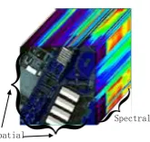
As the improvement of imaging spectrometers, hyperspectral remote sensing has developed rapidly as a new type of technology in earth observation. Imaging spectrometers which are often referred to as hyperspectral cameras, acquire the two-dimensional spatial information of the observation area as well as the electromagnetic energy scattered information in the spectral domain of the corresponding spatial position simultaneously. Thus the information stored is in the form of a three-dimensional data cube, which is shown as follows.

________________________________________

Spectral





_

Spatial

Figure 1. An example of hyperspectral data cube.

The hyperspectral remote sensing solves the problem that the imaging band is limited and it is difficult to form the curve of the detection area in the spectral dimension to analysis the characteristic of the materials in the corresponding area. They are widely used in the atmospheric analysis, exploration, environmental monitoring, and so on[1]. However, due to that the data is three-dimensional, new data processing technology should be researched to adapted to the character, especially the effective visualization methods. Since the display screen is two dimensional, the significant research in hyperspectral data visualization is to map the data cube to the screen.

An intuitive way to visual hyperspectral data is to turn it to an imaging display problem in the spatial domain, and the traditional researches mainly focused on visualizing hyperspectral data through color images. The hyperspectral cameras can obtain nearly continuous curves in the spectral domain for the spatial points, so the images which are to be displayed according to different spectral channels are in a large numbers which may reach to dozens or even hundreds. Unfortunately, the color image just has three color channels as well as a transparency component, so it is a great challenge to visual the hyperspectral data with such a large number of channels in the spectral domain by color images.

classification and so on. In[5], a color visualization model based on sparse coding was proposed for hyperspectral image. In this paper, the hyperspectral data was represented by sparse coding and then the codes were mapped to different colors and the corresponding image was displayed. Wang Cailing et al.[6] also proposed three methods to combine the data of different spectral channels to three color components based on the Fourier transformation, features of interference data and human visual system respectively.

In addition to visualize the original hyperspectral data, there are some studies that visualize the processing results for special applications. For example, in[7], hyperspectral images were used in corn seeds identification and the final results were displayed by the visualization technology.

The algorithms reviewed above either fuse the spectral channels or performed principal component analysis to reduce the number of channels to less than three and then visualize the hyperspectral data by color images. However, the pre-processing by fusion or principal component analysis should lose some information of the data, so the ability to display the features of the raw hyperspectral data is relatively limited.

In this paper, we focus on the visualization of the raw hyperspectral data and propose an interaction method to visual hyperspectral data in the two dimensional spatial domain and one dimensional spectral domain separately. The piecewise linear interpolation method is studied to map different hyperspectral values to different colors. An interaction method is proposed to visual the isosurface which shows the distribution of the chosen value in the hyperspectral data cube both in the spatial and the spectral domain. To some extent, the proposed visualization method displays the features of the original hyperspectral data and can be beneficial to noise analysis and spectral channel analysis for users. Since the proposed method visuals the raw hyperspectral data which avoids information loss during pre-processing, the characteristics of the original data are presented directly to the data users.

This paper is organized as follows: in section 2, an interactive visualization framework for the spatial domain and the spectral domain is researched. Then the visualization method for isosurface of the hyperspectral data is proposed in section 3. The visual results are displayed in section 4 to show the efficiency of the proposed methods. We conclude the whole paper in section 5.

INTERACTIVE VISUALIZATION METHOD FOR HYPERSPECTRAL DATA IN SPATIAL AND SPECTRAL DOMAIN

Since the hyperspectral cube data are three dimensional whereas the computer screen is two dimensional. An intuitive way is to fix the channel in the spectral domain and show the spatial data according to the specific spectral channel or fix the spatial position and show the spectral curve of the given spatial position. The specified values can be acquired by an interaction framework. According to the characteristics as well as the physical meaning of hyperspectral data, visualization by color images in two-dimensional spatial domains and curves in one-dimensional spectral domain is studied in this section.

Let H𝑀×𝑁×𝑃 be the hyperspectral data, where 𝑀 × 𝑁 is the size in the spatial domain and 𝑃 is the number of spectral bands of the hyperspectral data.

INTERACTIVE VISUALIZATION OF THE SPECTRAL CURVE

A hot topic in hyperspectral analysis is to identify materials in spatial domain based on the spectral characters. In this subsection, a two-line interaction framework is proposed to enable users to tune the spatial point in an intuitive way. After the spatial location is selected, the corresponding spectral information can be shown in the screen.

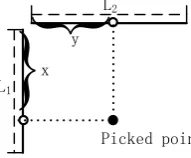
Let the length of the interactive line in the spatial domain be 𝐿₁ and 𝐿₂ respectively. The distances between the picked point and the initial points of the lines are 𝑥 and 𝑦 in the two directions respectively, just as shown in Figure 2.

Figure 2. Sketch map of two-line interaction framework.

The corresponding spatial coordinate can be obtained by the following equations.

𝑚𝑓 = ⌊𝑀 ×_𝐿𝑥

1⌋ （1）

𝑛𝑓 = ⌊𝑁 ×_𝐿𝑦

2⌋ （2）

In which, ⌊∙⌋ is the symbol to compute the round down of the given number to get the largest integer less than it. After obtaining the corresponding index in the spatial domain based on interaction, a vector in the spectral domain can be acquired with dimension 𝑃 × 1. Let 𝐹_𝑃×1 be the vector which we should visualized, so

𝐹_𝑃×1 = 𝐻(𝑚𝑓, 𝑛𝑓,∙) （3）

The vector can be displayed by a curve in the screen, wherein the axes are the spectral channels and scattered electromagnetic energy respectively. The values in 𝐹_𝑃×1 are connected by straight line to form the whole curve. If the position is changed by users, the corresponding position 𝑥 and 𝑦 will be modified and we recalculate the spatial point. Finally the spectral vector is updated and visualized.

The above visualization method fixes the spatial position of the hyperspectral data and displays the spectral curves. In the same way, the spectral index can be fixed and the according spatial information can be displayed by color mapping.

L2

L1



y



x

MAINTAININGTHEINTEGRITYOFTHESPECIFICATIONS

There are two problems which should be solved before we visualize the hyperspectral data in the form of spatial image. One is to design an interaction method to fix the spectral channel and the other is to map the values in the spatial domain to different colors. The first problem can be solved by the line interaction method. A line interaction method will be used to determine the spectral channel to be displayed by color image. And the index of the spectral channel can be computed by the point selected by users.

Assume that the length of interaction line is L₃ and the distance between point that users selected and the original point of the line is z. The corresponding spectral channel can be calculated by:

𝑝𝑓 = ⌊P ×_𝐿𝑧

3⌋ （4）

Once the spectral channel is determined, the corresponding data in the spatial domain for the hyperspectral data cube can be extracted. The data should be stored in the form of two dimensional matrix S_𝑀×𝑁 with size 𝑀 × 𝑁.

𝑆𝑀×𝑁 = 𝐻(∙,∙, pf) （5）

The matrix can be visualized by mapping each element to the pixel of the screen. An adaptive way is that the mapping color can be set by users according to different visualization requirements. In this study, the hyperspectral values are mapped to different colors by piecewise linear interpolation.

Let 𝑐𝑛 be the number of the control points set by the users, and

{(𝑎𝑖, 𝑐𝑖)𝑖=1,2,…,𝑐𝑛} be the control points, in which 𝑎𝑖 is the value of the hyperspectral data with index i among the control point and 𝑐_𝑖 is the color corresponding to 𝑎_𝑖. The color may be grey with just one component or be a triple with three primary components as 𝑐_𝑖 = (𝑐_𝑖,𝑅, 𝑐_𝑖,𝐺, 𝑐_𝑖,𝐵) . Finally the elements S(𝑚, 𝑛) of matrix S_𝑀×𝑁 are mapped to differnet pixels of the screen with different colors calculated by the value of S(𝑚, 𝑛). The colors are calculated by

XC(m, n)_𝑅 = c𝑖+1,𝑅−c𝑖,𝑅

a𝑖+1−a𝑖 (𝑆(𝑚, 𝑛) − a𝑖)+c𝑖,𝑅, a𝑖 < 𝑆(𝑚, 𝑛) < a𝑖+1 （6）

XC(m, n)_𝐺 =c𝑖+1,𝐺−c𝑖,𝐺

a𝑖+1−a𝑖 (𝑆(𝑚, 𝑛) − a𝑖)+c𝑖,𝐺, a𝑖 < 𝑆(𝑚, 𝑛) < a𝑖+1 （7）

XC(m, n)_𝐵 = c𝑖+1,𝐵−c𝑖,𝐵

XC(m, n) = (XC(m, n)_𝑅, XC(m, n)_𝐺, XC(m, n)_𝐵) （9）

The hyperspectral data can be visualized by setting the screen pixels to the calculated colors.

VISUALIZATIONMETHODFORISOSURFACEOFTHE

HYPERSPECTRALDATA

The hyperspectral data visualization method studied in the above section would reduce the dimension of the data cube which cannot be shown by the two dimensional screen by fixing the spatial coordinates or the spectral channels. But the method does not make full advantage of the hyperspectral data which combine the spatial as well as the spectral information together in sensing.

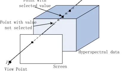
Therefore, it is necessary to focus on a visualization method which can effectively displays the distribution of hyperspectral data both in the spatial and spectral domain. The method proposed in this section makes use of the ray casting algorithm to visualize the distribution of the value specified by the users. The color 𝑅𝐶 according to the specified value is calculated by the piecewise linear interpolation just as mentioned above and the next step is to get the points to be shown in the data cube based on the users’ specified value.

Assume the value to be displayed is 𝑣𝑎𝑙, the principle of the visualziation is shown by the following figure.

Screen

Hyperspectral data Point with

selected value

View Point Point with value

not selected

Figure 3. Principle of the proposed method.

In order to take a good view of the hyperspectral data, a disturbance is given to the users’ specified value 𝑣𝑎𝑙. Let the agitating coefficient be a, the range of the hyperspectral data to be visualized is within the interval 𝑅_𝑣𝑎𝑙 = (𝑣𝑎𝑙 −

𝑎(𝐻_𝑚𝑎𝑥 − 𝐻_𝑚𝑖𝑛), 𝑣𝑎𝑙 + 𝑎(𝐻𝑚𝑎𝑥− 𝐻𝑚𝑖𝑛)). Assume a ray is emitted from the view point to the data cube. The ray may intersects with the screen and the intersection point is (𝑖, 𝑗), and at the same time intersects with the hyperspectral data. We resample the points in the data cube along the ray with distance δ and calculate the sampling values. If the sampling value is in 𝑅_𝑣𝑎𝑙, the screen pixcel

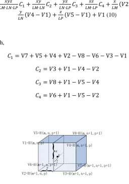
adjacent points of the hyperspectral data in the three dimension(𝐿𝑀 and 𝐿𝑁 in the spatial dimension and 𝐿𝑃 in the spectral dimension). 𝑉𝐻 can be calculated as follows.

VH =_{𝐿𝑀∙𝐿𝑁∙𝐿𝑃}𝑥𝑦𝑧 𝐶₁+_{𝐿𝑀∙𝐿𝑁}𝑥𝑦 𝐶₂+_{𝐿𝑁∙𝐿𝑃}𝑦𝑧 𝐶₃ +_{𝐿𝑀∙𝐿𝑃}𝑥𝑧 𝐶₄+_𝐿𝑀𝑥 (𝑉2 − 𝑉1) +

𝑦

𝐿𝑁(𝑉4 − 𝑉1) + 𝑧

𝐿𝑃(𝑉5 − 𝑉1) + 𝑉1 (10)

in which,

𝐶1 = V7 + V5 + V4 + V2 − V8 − V6 − V3 − V1

𝐶₂ = 𝑉3 + 𝑉1 − 𝑉4 − 𝑉2

𝐶3 = 𝑉8 + 𝑉1 − 𝑉5 − 𝑉4

𝐶4 = 𝑉6 + 𝑉1 − 𝑉5 − 𝑉2

Figure 4. Compute the value VH of the sample point V.

The proposed algorithm can be described below.

Input: O𝑅(Position of view point), 𝑣𝑎𝑙 (range of values to be visualized), H𝑀×𝑁×𝑃 (hyperspectral data), 𝑅𝐶 (color to be displayedδ(sample interval), for the

specified value), 𝐵𝐶 (background color).

Output: PC𝑋×𝑌.(color according to each pixels in the screen)

Step 1: for each pixel (𝑖, 𝑗) in the screen, _{the background color} 1 ≤ 𝑖 ≤ 𝑋, 1 ≤ 𝑗 ≤ 𝑌_{PC(𝑖, 𝑗) = 𝐵𝐶}, set the pixel color to _.

Step 2: _{data cube, turn to} Emit a line from view point to pixel_{Step 1. If the line intersects with the data cube, go to} (𝑖, 𝑗), if the line does not intersect with the _{Step 3.}

Step 3: _{sample points (}Calculate the first and last intersect points _{NS) and the position PS} 𝑆𝑃 and 𝐸𝑃. Get the number of the

𝑁𝑆×1 according to the sample interval δ

Step 4: for the sample point PS(k), 1 ≤ k ≤ NS

Step 5: Calculate the sample value VH(k) by formula (10)

V2=H(m+1,n,p) V3=H(m+1,n+1,p)

V1=H(m,n,p)

V4=H(m,n+1,p) V8=H(m,n+1,p+1) V5=H(m,n,p+1)

V6=H(m+1,n,p+1) _{V7=H(m+1,n+1,p+1)}



x



y

Step 6: If VH(k)_{in the screen to the specific color} is not in the interval 𝑅𝑣𝑎𝑙, turn to _{PC(𝑖, 𝑗) = 𝑅𝐶}Step 4, else set the pixel _{, go to Step 1}(𝑖, 𝑗) end for

end for

The algorithm described above visualizes the specified hyperspectral value by the corresponding color which both consider the spatial and the spectral dimension. In other words, we visualize the isosurface in the hyperspectral data. We can conclude for Step 6 that once the pixel color is set, the algorithm stop to the next pixel in the screen but not compute the values of all the sample points, which saves time to some extent. The background color 𝐵𝐶 is always set to white (255,255,255) or black (0,0,0). In the experimental section, the background color is set to white, that is to say, if the view line is not interacted with the hyperspectral data, the pixel that the view line interact with the screen is set to white.

EXPERIMENTALRESULTS

In this section, the visualization results for different hyperspectral datasets are given. The results include visualization in the spatial domain, visualization in the spectral domain and visualization the isosurface in the hyperspectral data. Before we show the results, the datasets used in this section are given.

TABLEI.HYPERSPECTRALDATASETUSEDINTHISSECTION.

NO. Spectrometers Size Details

1

Airborne visible/Infrared Imaging Spectrometer

(AVIRIS)

200 × 200 × 96 Area Around Santiago

Airport

2

Airborne visible/Infrared Imaging Spectrometer

(AVIRIS)

145 × 145 × 200 Indian Pines

3

ROSIS-03 (Reflective Optical System Imaging

Spectrometer)

256 × 256 × 103 Pavia University

VISUALIZATION BY SPECTRAL CURVE

(a)(131,129) (b) (117,151) (c) (79,192)

20 40 60 80 100 120 140 160 180 200 20

40 60 80 100 120 140 160 180 200

（131,129） （117,151） （79,192） （38,64）

(d) (38,64) (e)points of (a)(b)(c) and (d)

Figure 5. Interactive visualization results based on curves of Dataset 1. (a)-(d) are the spectral curves according to different spatial positions marked by (e).

In Figure 5(e), the four points are similar in this spectral channel, but from Fig 5(a)(b)(c)(d), we can conclude that the spatial points (131,129), (117,151) and (79,192) are similar since the curves are not distinguished from each other too much, but point (38,64) is quite different. This is the advantage to show the hyperspectral data in the spectral domain.

Figure 6 shows the visualization results in the spectral domain for Dataset 2.

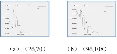
（a）（26,70） （b）（96,108）

Figure 6. Interactive visualization results based on curves of Dataset 2. (a)-(b) are the spectral curves according to different spatial positions.

We can conclude from the visualization results that the spectral curve has many troughs, that is, the absorption of energy in these channels is much higher than others. The reason may be that the atmosphere absorbs the energy of certain channels.

VISUALIZATIONBYSPATIALIMAGES

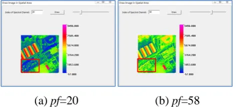
(a) pf=20 (b) pf=58

Figure 7. Interactive visualization results based on spatial images of Dataset 1. (a)-(b) are the images according to different spectral channels 20 and 58.

The slider in the upper right corner of the dialog allows the users to select the spectral channel to be shown interactively. The right side of the figure shows the color bar which maps the reflection values to different colors.

The map function can be changed by tune the black triangles shown as follows.

Figure 8. Color bar to change the map function between the values and colors.

The interactive visualization base on spatial images of Dataset 3 is shown in Figure 9.

(a) pf=21 (b) pf=73

Figure 9. Interactive visualization results based on spatial images of Dataset 3. (a)-(b) are the images according to different spectral channels 21 and 73.

The visualization method of the spatial domain shows the characteristic of different spectral channels much clear. For example, the distinction of the target in area marked red rectangle is much easier when pf=20 than pf=58 in Dataset 1, while in Dataset 3, the area marked in red rectangles is much more distinguishable when pf=73 than pf=21. Obviously, Figure 9(b) shows much more details than Figure 9(a) in the red rectangle.

INTERACTIVEVISUALIZATIONOFISOSURFACEIN

HYPERSPECTRALDATA

interval is set to δ = 0.383. The visualization of the data according to different values is shown in Figure 10.

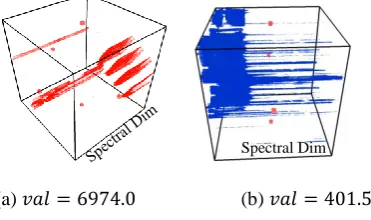
(a) 𝑣𝑎𝑙 = 6974.0 (b) 𝑣𝑎𝑙 = 401.5

Figure 10. Interactive visualization results based on Isosurface of Dataset 1 with values 6974.0 and 401.5.

As we can see from Figure 10(a), there is a large amount of noise when the data value is around 6974.0 because there are a lot of red points in the visualization result. Additionally, there are some regions with similar values when the indexes of the channels are small, however, as the index increases, some spatial position maintained the same value while the values of other area change. In the visualization results, the red color appears through the spectral channel in some positions, on the contrary, in some positions the red color vanishes because the according values are out of the visualization range. Figure 10 (b) shows that the positions with value 401.5 are mainly concentrated in channels with small indexes.

The visualization of Dataset 2 based on isosurface is shown in Figure 11. The perturbation coefficient 𝑎 = 8 × 10−5, and the sample interval is set to δ =

0.237.

(a) 𝑣𝑎𝑙 = 1681.5 (b) 𝑣𝑎𝑙 = 6401.5 (c) 𝑣𝑎𝑙 = 3445.9

Figure 11. Interactive visualization results based on isosurface of Dataset 2 with values 1681.5, 6401.5 and 3445.9.

We can conclude from Figure 11 that the data just concentrates to several channels for a specific value. For example, if the value is 𝑣𝑎𝑙 = 1681.5, there are three channel intervals with this value, while there are just one channel interval with value 6401.5. The value 3445.9 in Dataset 2 concentrated to four channel intervals as shown in Figure 11(c).

We also visualize Dataset 3 by the proposed algorithm shown as follows. The perturbation coefficient 𝑎 = 8 × 10−5, and the sample interval is set to δ =

0.403.

Spectral Dim

（a）𝑣𝑎𝑙 = 5088.0 （b）𝑣𝑎𝑙 = 3936.0 （c）𝑣𝑎𝑙 = 2848.0

Figure 12. Interactive visualization results based on Isosurface of Dataset 3 with values 5088.0, 3936.0 and 2848.0.

It is concludes from Figure 12 that there are some noise in the data cube with value 5088.0, as well as the region with this value is quite small. The region increases when the value reduced to 3936.0. And when the value is turned to 2848.0, the region keeps on growing.

This visualization method shows the distribution of the data values in the hyperspectral cube in an intuitive way to the data users. Besides, the rendering times for the three data are less than 0.04s in our experiments in the computer equipped with four cored i5-4590 CPU and thus can be used in real time visualization.

CONCLUSION

Aiming at the visualization of hyperspectral data, this paper researched on an interactive frame work to show the data in the spatial and spectral domain by fixing the position or the channel. A visualization method was proposed to show the values in the whole data cube which displayed the distribution of the specified value in the raw hyperspectral data. The advantage of the proposed method is that the spatial and spectral information in the original data are shown simultaneously in the screen while the other reviewed algorithms did the dimension reduction and showed the data by just one color image which may cause loss of information. For further research, we will concentrate on visualize the hyperspectral data by the volume rendering method and solve the problem of overlapping when map to the screen.

ACKNOWLEDGEMENTS

REFERENCES

1. José M. Bioucas-Dias, Antonio Plaza, Nicolas Dobigeon, Mario Parente, Qian Du, Paul Gader, and Jocelyn Chanussot, “Hyperspectral Unmixing Overview: Geometrical, Statistical, and Sparse Regression-Based Approaches”. IEEE Journal of Selected Topics in Applied Earth Oservation and Remote Sensing. 2012.5(2):354-379.

2. Liu Danfeng， Wang Liguo, Zhao Liang, “Dynamic display of the hyperspectral image synchronized colors”, Journal of Harbin Engineering University, 2014.35(6):760-765. 3. Wang Liguo, Wu Fei．“KL-ISOMAP-based color visualization for hyperspectral

imagery”. Journal of Nanjing University of Information Science and Technology (Natural Science Edition) ，2018, 10(1): 63-71.

4. Wang Liguo, Liu Danfeng, Zhao Liang. “Distance-Preserving Color Visualization Model for Hyperspectral Imagery”. 2013.31(1):72-78.

5. Wang Li-Guo, Liu Dan-Feng, and Zhao Liang. “Sparse representation-based color visualization methodor hyperspectral imaging”. Applied Geophysics. 2013.10(2):210-221.

6. Wang Cailing, Li Yushan, Liu Xuebn, et.al. “Spatial Domain Display for Interference Image Dataset”. Spectroscop and Spectral Analysis. 2011.31(11):3158-3162.