Multigrid Method for the Numerical Solution of the Modified Equal Width Wave Equation

http://dx.doi.org/10.4236/am.2016.710102

Multigrid Method for the Numerical Solution

of the Modified Equal Width Wave Equation

Yasser M. Abo Essa

Mathematics Department, Faculty of Education and Science (AL-Khurmah Branch), Taif University, Taif, Kingdom of Saudi Arabia

Received 3 April 2016; accepted 21 June 2016; published 24 June 2016

Copyright © 2016 by author and Scientific Research Publishing Inc.

This work is licensed under the Creative Commons Attribution International License (CC BY). http://creativecommons.org/licenses/by/4.0/

Abstract

Numerical solutions of the modified equal width wave equation are obtained by using the multi-grid method and finite difference method. The motion of a single solitary wave, interaction of two solitary waves and development of the Maxwellian initial condition into solitary waves are studied using the proposed method. The numerical solutions are compared with the known analytical

so-lutions. Using L L2, ∞ error norms and conservative properties of mass, momentum and energy,

accuracy and efficiency of the mentioned method will be established through comparison with other methods.

Keywords

Multigrid Method, Finite Difference Method, MEW Equation

1. Introduction

A large system of equations comes out from discretization of the domain of partial differential equations into a collection of points and the optimal method for solving these problems is multigrid method, see [1]-[4].

The modified equal width wave (MEW) equation introduced by Morrison et al. [5] is used as a model equa-tion to describe the nonlinear dispersive waves. Gardner and Gardner [6] [7] solved the EW equaequa-tion with the Galerkin’s method using cubic B-splines as a trial and test function. The MEW equation was similar with the modified regularized long wave (MRLW) equation [8] and modified Korteweg-de Vries (MKdV) equation [9]. All the modified equations are nonlinear wave equations with cubic nonlinearities and all of them have solitary wave solutions, which are wave packets or pulses. These waves propagate in non-linear media by keeping wave forms and velocity even after interaction occurs.

solutions are based on septic B-spline finite elements and Petrov-Galerkin finite element method with weight functions quadratic and element shape functions which are cubic B-splines. Esen [12] [13] solved the MEW eq-uation by applying a lumped Galerkin method based on quadratic B-spline finite elements. Saka [14] proposed algorithms for the numerical solution of the MEW equation using quintic B-spline collocation method. Zaki [15] considered the solitary wave interactions for the MEW equation by collocation method using quintic B-spline finite elements and obtained the numerical solution of the EW equation by using least-squares method [16]. Wazwaz [17] investigated the MEW equation and two of its variants by the tanh and the sine-cosine methods. A solution based on a collocation method incorporated cubic B-splines is investigated by Saka and Dağ [18]. Lu [19] presented a variational iteration method to solve the MEW equation. Evans and Raslan [20] studied the ge-neralized EW equation by using collocation method based on quadratic B-splines to obtain the numerical solu-tions of a single solitary waves and the birth of solitons. Esen and Kutluay [21] studied a linearized implicit fi-nite difference method in solving the MEW equation. Battal Gazi Karakoc and Geyikli [22] solved the MEW equation by a lumped Galerkin method using cubic B-spline finite elements.

An outline of this paper is as follows: We begin in Section 2 by reviewing the analytical solution of the MEW equation. In Section 3, we derive a new numerical method based on the multigrid technique and finite difference method for obtaining the numerical solution of MEW equation. Finally, in Section 4, we introduce the numerical results for solving the MEW equation through some well known standard problems.

2. The Analytical Solution

The modified equal width wave equation which is as a model for non-linear dispersive waves, considered here has the normalized form [5]

2

3 0,

t x xxt

u + u u −

µ

u = (1) with the physical boundary conditions u→0 as x→ ±∞, where t is time and x is the space coordinate, µ is a positive parameter. For this study boundary conditions are chosen

( )

( )

( )

( )

( )

( )

, 0, , 0,

, 0, , 0,

, 0, , 0,

x x

xxt xxt

u a t u b t

u a t u b t

u a t u b t

= =

= =

= =

(2)

and the initial condition as

( )

, 0

( )

, ,

u x = f x a≤ ≤x b where f is a localized disturbance inside the considered interval.

The exact solution of equation (1) can be written in the form [15]

( )

, sech

(

(

0

)

)

,

u x t =A P x−x −νt (3) which represents the motion of a single solitary wave with amplitude A, where the wave velocity

ν

=A2 2

and P= 1µ. The initial condition is given by

( )

, 0 sech

(

(

0

)

)

u x =A P x−x (4) For the MEW equation, it is important to discuss the following three invariant conditions given in [15], which, respectively, correspond to conversation of mass, momentum, and energy. The analytical values of the inva-riants are

2 2 4

1 2 3

π 2 2 4

, , .

3 3

A A PA A

C C C

P P P

µ

= = + = (5)

3. Numerical Method

partial differential equation at time t1 and use these solutions as initial values for the next level u x

( )

, 0 =u x t

( )

,1 , and for the other, we obtain the solutions at time T. The numbers of points in a coarse grid for this domain are two points.

We apply the full multigrid algorithm for the MRLW equation. Assuming the initial condition

( )

, 0

( )

u x = f x and the solution u x t

( )

, , a≤ ≤x b, 0≤ ≤t T has the usual partition with a space step size x

∆ and a time step size ∆t (tK+₁=tK + ∆t K, =0,1, 2,).

We start handling the non-linear term 3u u2 x by expressing in the form

3 u

x ∂

∂ . The back-time and centre- space difference for Equation (1) is

( ) ( )

(

) (

) (

)

( ) ( )

3 3

1, 1, 1, 1, 1 , , 1 1, 1, 1

, , 1

2

2

0, 2

k k k k k k k k

k k

i n i n i n i n i n i n i n i n

i n i n u u u u u u u u

u u

t x x t

µ

+ − + + − − − − −

− − − − − + −

−

+ − =

∆ ∆ ∆ ∆ (6)

where 1, , 2k 1, 1, , 2k

i=  − n=  , k=1,,M for a set grids 1, 2, , M.

G G  G

Step 1: K=0,u x

( )

, 0 = f x

( )

.

Step 2: Starting from k=1 in the coarse grid, we can calculate the approximate value u_{i n,} at two points using Equation (5) leading to:

( )

(

)

(

)

( )( )

(

( ) ( )

)

1 1 1 1 1 1

, , 1 ₂ 1, 1, 1, 1 1, 1

3 3 1 1 1, 1, 1 2 2 4

; 1, 1, 2.

i n i n i n i n i n i n

i n i n

u u u u u u

x

x t u u i n

µ µ − + − + − − − + −  = + _ + − − ∆ +  − ∆ ∆ − = =  (7)

The right hand side for equation (7) can be computed using the initial and boundary conditions.

Step 3: Interpolating the grid functions from the coarse grid to fine grid using linear interpolation I_kk+1, in which

1 1

,

k k k

k

u+ =I +u (8) that can be written explicitly as:

(

)

(

)

(

)

1 2 ,2 ,

1

2 1,2 , 1,

1

2 ,2 1 , , 1

1

2 1,2 1 , 1, , 1 1, 1

; 1, , 2 1, 1, , 2 ,

0.5 ; 0, , 2 1, 1, , 2 ,

0.5 ; 1, , 2 1, 0, , 2 1,

0.25 ; , 0, , 2 1.

k k k k

i n i n

k k k k k

i n i n i n

k k k k k

i n i n i n

k k k k k k

i n i n i n i n i n

u u i n

u u u i n

u u u i n

u u u u u i n

+ + + + + + + + + + + + + + = = − = = + = − = = + = − = − = + + + = −        (9)

Step 4: Doing relaxation sweep on Gk+1 using the point relaxation

( )

(

)

(

)

( )( )

(

( ) ( )

)

1

, , 1 ₂ 1, 1, 1, 1 1, 1

3 3 1 1 1, 1, 1 2 2 4

; 1, , 2 1, 1, , 2 .

k k k k k k

i n i n i n i n i n i n

k k k k

i n i n

u u u u u u

x

x t u u i n

µ µ + − + − + − − − + + + −  = + _ + − − ∆ +  − ∆ ∆ − = − =    (10)

Step 5: Computing the residuals k1

r + on k1

G + and inject them into k

G using full weighting restriction

1

k k

I + to get rk as:

1 1 ,

k k k

k

r =I ₊r + (11)

(

)

1 1 1 1

, 2 1,2 1 2 1,2 1 2 1,2 1 2 1,2 1

1 1 1 1 1

2 ,2 1 2 ,2 1 2 1,2 2 1,2 2 ,2

1 16

2 4 ; , 1, , 2 1.

k k k k k

i n i n i n i n i n

k k k k k k

i n i n i n i n i n

r r r r r

r r r r r i n

+ + + + − − − + + − + + + + + + + − + − +  = _ + + +  + + + + + _ =  − (12)

Step 7: Interpolating the solution of error ek onto Gk+1, ek 1 Ikk 1ek,

+ ₌ +

and adding it to uk+1 which is the approximate value of u on the fine grid with k=2.

By taking this solution on coarse grid and repeating steps 3-7, we obtain the approximate values of u on the grid with k=3 and so k=4, 5,,M the final value is the solution at the time level K+1.

Step 8: K=K+1, go to step 2 (lead to the solution at higher time level as needed).

4. Numerical Results

In this section, numerical solutions of MRLW equation are obtained for standard problems as: the motion of single solitary wave, interaction of two solitary waves and development of Maxwellian initial condition into so-litary waves. For the MEW equation, it is important to discuss the following three invariant conditions given in [15], which respectively correspond to conversation of mass, momentum and energy:

( )

(

)

( )

(

( )

)

( )

1 , 1 2 2 2 2

2 , ,

1 4 4 3 , 1 d , d , d . N b i n a i N b

x i n x i n

a i N b i n a i

C u x x u

C u u x x u u

C u x x u

µ µ = = = = = ∆   = + = ∆ _ + _   = = ∆

∑

∫

∑

∫

∑

∫

(13)

The accuracy of the method is measured by both the L₂ error norm

( )

2

2 ₂

0

, N

exact exact

N i N i

i

L u u x u u

=

= − = ∆

∑

− (14)

and the L∞ error norm

( )

max ,

exact exact

N _i i N i

L_∞ u u u u

∞

= − = − (15)

to show how good the numerical results in comparison with the exact results.

4.1. The Motion of Single Solitary Wave

Consider Equation (1) with boundary conditions (2) and the initial condition (4). For a comparison with earlier studies [13] [19] [21] [22] we take the parameters ∆ =x 0.1,∆ =t 0.05,µ=1,x₀ =30 and A=0.25 over the interval [0, 80]. To find the error norms L₂, L_∞ and the numerical invariants C C₁, ₂ and C₃ at various times we use the numerical solutions by applying the multigrid method up to t=20. As reported in Table 1, the error norms L₂, L_∞ are found to be small enough, and the computed values of invariants are in good agreement with their analytical values C₁=0.7853982,C₂=0.1666667,C₃=0.0052083. Table 2 shows a comparison of the values of the invariants and error norms obtained by the present method with those obtained by other methods [13] [19] [21] [22]. It is clearly seen from Table 2 that the error norms obtained by the present method are smaller than the other methods.

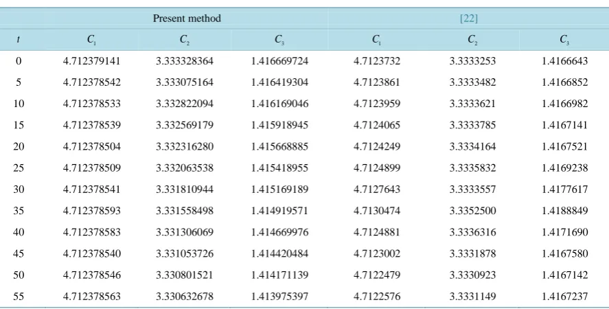
4.2. Interaction of Two Solitary Waves

Consider the interaction of two positive solitary waves as a second problem. For this problem, the initial condi-tion is given by:

( )

2

(

(

)

)

1

, 0 jsech j .

j

u x A P x x

=

=

∑

− (16)

For the computational discussion, firstly we use parameters ∆ =x 0.1,∆ =t 0.025,µ=1,A₁=1, A2=0.5,x1=15 and x₂=30 over the range

[

0, 80 to coincide with those used in [22].

]

In [20] the analytic invariants are C₁=π

(

A₁+A₂

)

=4.7123889,

( )

(

2 2

)

2 8 3 1 2 3.3333333

C = A +A = ,

( )

(

4 4

)

3 4 3 1 2 1.4166667

C = A +A = . The experiment is run from t=0 to t=55 and values of the invariant quantities C C₁, ₂ and C₃ are listed in Table 3.

[image:5.595.83.541.105.321.2]

Table 1. Invariants and error norms for single solitary wave when A=0.25,∆ =x 0.1,∆ =t 0.05,0≤ ≤x 80.

t C1 C2 C3

5 2 10

L× _{L 10}5

∞×

0 0.7853966199 0.1666662968 0.005208333331 0.000000000 0.000000

2 0.7853966246 0.1666660511 0.005208317956 0.0518705479 0.05440

4 0.7853966176 0.1666658044 0.005208302547 0.1038794545 0.10890

6 0.7853966097 0.1666655554 0.005208286962 0.1560469898 0.16359

8 0.7853966066 0.1666653078 0.005208271505 0.2080329043 0.21810

10 0.7853966012 0.1666650571 0.005208255823 0.2601313073 0.27283

12 0.7853965918 0.1666648091 0.005208240334 0.3122731279 0.32747

14 0.7853965793 0.1666645594 0.005208224692 0.3643751855 0.38216

16 0.7853965769 0.1666643124 0.005208209260 0.4164201991 0.43656

18 0.7853965785 0.1666640667 0.005208193877 0.4684782742 0.49095

[image:5.595.89.539.338.456.2]

20 0.7853965668 0.1666638167 0.005208178255 0.5208044265 0.54566

Table 2. Comparison of errors and invariants for single solitary wave at t=20.

Method C1 C2 C3

5 2 10

L× 5

10 L∞×

Analytical 0.7853982 0.1666667 0.0052083 0 0

Present 0.7853966 0.1666638 0.0052082 0.520804 0.54566

[13] 0.7853898 0.1667614 0.0052082 7.969400 4.65523

[19] 0.7849545 0.1664765 0.0051995 29.05166 24.98925

[21] 0.7853977 0.1664735 0.0052083 26.92812 25.69972

[22] 0.7853967 0.1666663 0.0052083 8.009800 4.606180

Table 3. Comparison of invariants for the interaction of two solitary waves with results from [22] (∆ =x 0.1,∆ =t 0.025,

1 1, 2 0.5,0 80

A = A = ≤ ≤x ).

Present method [22]

t C₁ C₂ C₃ C₁ C₂ C₃

0 4.712379141 3.333328364 1.416669724 4.7123732 3.3333253 1.4166643

5 4.712378542 3.333075164 1.416419304 4.7123861 3.3333482 1.4166852

10 4.712378533 3.332822094 1.416169046 4.7123959 3.3333621 1.4166982

15 4.712378539 3.332569179 1.415918945 4.7124065 3.3333785 1.4167141

20 4.712378504 3.332316280 1.415668885 4.7124249 3.3334164 1.4167521

25 4.712378509 3.332063538 1.415418955 4.7124899 3.3335832 1.4169238

30 4.712378541 3.331810944 1.415169189 4.7127643 3.3333557 1.4177617

35 4.712378593 3.331558498 1.414919571 4.7130474 3.3352500 1.4188849

40 4.712378583 3.331306069 1.414669976 4.7124881 3.3336316 1.4171690

45 4.712378540 3.331053726 1.414420484 4.7123002 3.3331878 1.4167580

50 4.712378546 3.330801521 1.414171139 4.7122479 3.3330923 1.4167142

[image:5.595.94.538.495.720.2]

[22]. It is seen that the numerical values of the invariants remain almost constant during the computer run. Finally, we have studied the interaction of two solitary waves with the following parameters ∆ =x 0.1,

1 2 1

0.025, 1, 2, 1, 15

t µ A A x

∆ = = = − = = and x₂=30 in the range [0,150].

[image:6.595.89.540.265.455.2]

The analytical invariants can be found as in [22] C₁= −3.1415927, C₂=13.3333333, C₃=22.6666667. The experiment is run from t = 0 to t = 55 and values of the invariant quantities C₁,C₂ and C₃ are listed in

Table 4.

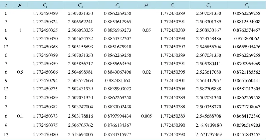
4.3. The Maxwellian Initial Condition

Last study, we consider the numerical solution of the equation (1) with the Maxwellian initial condition

( )

2

, 0 e x ,

u x = − (17) and the boundary conditions u

(

−20,t

)

=u_x

(

−20,t

)

=u

(

20,t

)

=u_x

(

20,t

)

=0.

Table 4. Invariants for the interaction of two solitary waves (∆ =x 0.1,∆ =t 0.025,A1= −2,A2=1, 0≤ ≤x 150).

t C₁ C2 C3

0 −3.141588324 13.33240988 22.66661773

5 −3.141587221 13.31632255 22.60298870

10 −3.141587293 13.30034113 22.53980538

15 −3.141587369 13.28446423 22.47706277

20 −3.141587465 13.26869077 22.41475674

25 −3.141587571 13.25301907 22.35288150

30 −3.141587642 13.23744806 22.29143237

35 −3.141587711 13.22197615 22.23040435

40 −3.141587744 13.20660137 22.16979117

45 −3.141587842 13.19132246 22.10958842

50 −3.141587954 13.17613770 22.04979002

[image:6.595.89.539.484.721.2]

55 −3.141587989 13.15897649 22.01765488

Table 5. Invariants of MEW equation using the Maxwelliancondition µ=1,0.5,0.1,0.05,0.02,0.005.

t µ C1 C2 C3 µ C1 C2 C3

0 1.772450389 2.507031350 0.8862269258 1.772450389 2.507031350 0.8862269258 3 1.772450324 2.506562241 0.8859617965 1.772450391 2.503301389 0.8812594008 6 1 1.772450355 2.506093335 0.8856969273 0.05 1.772450389 2.508930167 0.8763574457 9 1.772450370 2.505624532 0.8854322207 1.772450398 2.523558486 0.874805062 12 1.772450368 2.505155693 0.8851675910 1.772450397 2.546856704 0.8665905426

0 1.772450389 2.507031350 0.8862269258 1.772450389 2.507031350 0.8862269258 3 1.772450359 2.505856717 0.8855663594 1.772450391 2.505380411 0.8790965969 6 0.5 1.772450306 2.504698981 0.8849067496 0.02 1.772450395 2.523617080 0.8721185562 9 1.772450294 2.503557663 0.882481160 1.772450301 2.561417967 0.8651660441 12 1.772450275 2.502431939 0.8835903023 1.772450306 2.587705888 0.8581212805

0 1.772450389 2.507031350 0.8862269258 1.772450389 2.507031350 0.8862269258

3 1.772450382 2.503247004 0.8830002438 1.772450388 2.509358370 0.8771798047

6 0.1 1.772450373 2.503178816 0.8797994434 0.005 1.772450389 2.545688708 0.8684172340

9 1.772450375 2.506705762 0.8766134367 1.772450390 2. 619139180 0.8596519203

It is known that the behavior of the solution with the Maxwellian condition (17) depends on the values of µ. So we have considered various values for µ. The computations are carried out for the cases

µ

=1, 0.5, 0.1,

0.05, 0.02 and 0.005 which are used in the earlier papers [15] [19]. The numerical conserved quantities with

1, 0.5, 0.1, 0.05, 0.02

µ

= and 0.005 are given in Table 5. It is observed that the obtained values of the invariants remain almost constant during the computer run.

5. Conclusion

In this paper we study the MEW problem by extending the use of multigrid technique. We checked our scheme through single solitary wave in which the analytic solution is known. Our scheme was extended to study the in-teraction of two solitary waves and Maxwellian initial condition where the analytic solutions are unknown dur-ing the interaction. The performance and accuracy of the method were explained by calculatdur-ing the error norms

2,

L L∞ and conservative properties of mass, momentum and energy. The computed results showed that our

scheme is a successful numerical technique for solving the MEW problem and can be also efficiently applied for solving a large number of physically important non-linear problems.

References

[1] Brandt, A. (1977) Multi-Level Adaptive Solution to Boundary-Value Problem. Mathematics of Computation, 31, 333- 390. http://dx.doi.org/10.1090/S0025-5718-1977-0431719-X

[2] Abo Essa, Y.M., Amer, T.S. and Ibrahim, I.A. (2011) Numerical Treatment of the Generalized Regularized Long- Wave Equation. Far East Journal of Applied Mathematics, 52, 147-154.

https://www.researchgate.net/.../266611672

[3] Abo Essa, Y.M., Amer, T.S. and Abdul-Moniem, I.B. (2012) Application of Multigrid Technique for the Numerical Solution of the Non-Linear Dispersive Waves Equations. International Journal of Mathematical Archive, 3, 4903- 4910.

[4] Abo Essa, Y.M., Ibrahim, I.A. and Rahmo, E.-D. (2014) The Numerical Solution of the MRLW Equation Using the Multigrid Method. Applied Mathematics, 5, 3328-3334. http://dx.doi.org/10.4236/am.2014.521310

[5] Morrison, P.J., Meiss, J.D. and Cary, J.R. (1984) Scattering of Regularized-Long-Wave Solitary Waves. Physica D. Nonlinear Phenomena, 11, 324-336.http://dx.doi.org/10.1016/0167-2789(84)90014-9

[6] Gardner, L.R.T. and Gardner, G.A. (1990) Solitary Waves of the Regularized Long Wave Equation. Journal of Com-putational Physics, 91, 441-459.

[7] Gardner, L.R.T. and Gardner, G.A. (1992) Solitary Waves of the Equal Width Wave Equation. Journal of Computa-tional Physics, 101, 218-223. http://dx.doi.org/10.1016/0021-9991(92)90054-3

[8] Abdulloev, Kh. O., Bogolubsky, I.L. and Makhankov, V.G. (1976) One More Example of Inelastic Soliton Interaction.

Physics Letters. A, 56, 427-428. http://dx.doi.org/10.1016/0375-9601(76)90714-3

[9] Gardner, L.R.T., Gardner, G.A. and Geyikli, T. (1994) The Boundary Forced MKdV Equation. Journal of Computa-tional Physics, 113, 5-12.

[10] Geyikli, T. and Battal Gazi Karakoc, S. (2011) Septic B-Spline Collocation Method for the Numerical Solution of the Modified Equal Width Wave Equation. Applied Mathematics, 2, 739-749. http://dx.doi.org/10.4236/am.2011.26098

[11] Geyikli, T. and Battal Gazi Karakoc, S. (2012) Petrov-Galerkin Method with Cubic B-Splines for Solving the MEW Equation. Bulletin of the Belgian Mathematical Society - Simon Stevin, 19, 215-227.

http://projecteuclid.org/euclid.bbms/1337864268

[12] Esen, A. (2005) A Numerical Solution of the Equal width Wave Equation by a Lumped Galerkin Method. Applied Mathematics and Computation, 168, 270-282. http://dx.doi.org/10.1016/j.amc.2004.08.013

[13] Esen, A. (2006) A Lumped Galerkin Method for the Numerical Solution of the Modified Equal-Width Wave Equation Using Quadratic B-Splines. International Journal of Computer Mathematics, 83, 449-459.

http://dx.doi.org/10.1080/00207160600909918

[14] Saka, B. (2007) Algorithms for Numerical Solution of the Modified Equal Width Wave Equation Using Collocation Method. Mathematical and Computer Modeling, 45, 1096-1117. http://dx.doi.org/10.1016/j.mcm.2006.09.012

[15] Zaki, S.I. (2000) Solitary Wave Interactions for the Modified Equal Width Equation. Computer Physics Communica-tions, 126, 219-231. http://dx.doi.org/10.1016/S0010-4655(99)00471-3

[17] Wazwaz, A.-M. (2006) Thetanh and the Sine-Cosine Methods for a Reliable Treatment of the Modified Equal Width Equation and Its Variants. Communications in Nonlinear Science and Numerical Simulation, 11, 148-160.

http://dx.doi.org/10.1016/j.cnsns.2004.07.001

[18] Saka, B. and Dağ, İ. (2007) Quartic B-Spline Collocation Method to the Numerical Solutions of the Burgers’ Equation,

Chaos. Solitons and Fractals, 32, 1125-1137. http://dx.doi.org/10.1016/j.chaos.2005.11.037

[19] Lu, J. (2009) He’s Variational Iteration Method for the Modified Equal Width Equation. Chaos, Solitons and Fractals,

39, 2102-2109. http://dx.doi.org/10.1016/j.chaos.2007.06.104

[20] Evans, D.J. and Raslan, K.R. (2005) Solitary Waves for the Generalized Equal Width (GEW) Equation. International Journal of Computer Mathematics, 82, 445-455. http://dx.doi.org/10.1080/0020716042000272539

[21] Esen, A. and Kutluay, S. (2008) Solitary Wave Solutions of the Modified Equal Width Wave Equation. Communica-tions in Nonlinear Science and Numerical Simulation, 13, 1538-1546. http://dx.doi.org/10.1016/j.cnsns.2006.09.018

[22] Battal Gazi Karakoc, S. and Geyikli, T. (2012) Numerical Solution of the Modified Equal width Wave Equation. In-ternational Journal of Differential Equations, 2012, Article ID: 587208. http://dx.doi.org/10.1155/2012/587208