Multiresolution Finite Element Method
Based on a New Locking-Free Rectangular
Mindlin Plate Element
Yiming Xia
Department of Civil Engineering, College of Aerospace Engineering, Nanjing University of Aeronautics and Astronautics, Nanjing, China
Received 24 May 2016; accepted 21 June 2016; published 24 June 2016
Copyright © 2016 by author and Scientific Research Publishing Inc.
This work is licensed under the Creative Commons Attribution International License (CC BY).
http://creativecommons.org/licenses/by/4.0/
Abstract
A locking-free rectangular Mindlin plate element with a new multi-resolution analysis (MRA) is proposed and a new finite element method is hence presented. The MRA framework is formulated out of a mutually nesting displacement subspace sequence whose basis functions are constructed of scaling and shifting on the element domain of basic full node shape function. The basic full node shape function is constructed by extending the split node shape function of a traditional Mindlin plate element to other three quadrants around the coordinate zero point. As a result, a new ra-tional MRA concept together with the resolution level (RL) is constituted for the element. The tra-ditional 4-node rectangular Mindlin plate element and method is a mono-resolution one and also a special case of the proposed element and method. The meshing for the monoresolution plate ele-ment model is based on the empiricism while the RL adjusting for the multiresolution is laid on the rigorous mathematical basis. The analysis clarity of a plate structure is actually determined by the RL, not by the mesh. Thus, the accuracy of a plate structural analysis is replaced by the clarity, the irrational MRA by the rational and the mesh model by the RL that is the discretized model by the integrated.
Keywords
Rectangular Mindlin Plate Element, Split Node, Full Node, Analysis Clarity, Displacement Subspace Sequence, Rational Multiresolution Analysis, Resolution Level
1. Introduction
However, in the field of computational mechanics, the MRA has not been, in a real sense, fully utilized in the numerical solution of engineering problems either by the traditional finite element method (FEM) [1] or by other
methods such as the wavelet finite element method (WFEM) [2] [3], the meshfree method (MFM) [4]-[7] and
the natural element method (NEM) [8] [9] etc.
As is commonly known of the FEM, owing to the invariance of node number a single element contains the element that can be regarded as a monoresolution one from a MRA point of view and the FEM structural analy-sis is usually not associated with the MRA concept. The MRA seems to be rarely used when the FEM is em-ployed to numerical analysis. However, it is, in fact, by means of meshing and re-meshing in which a cluster of monoresolution finite elements are assembled together artificially that the rough MRA is executed by the FEM. As we can see, in overall analysis process of a structure by the FEM, there is no mathematical foundation for the traditional finite element meshing and the finite elements are assembled together artificially. The traditional fi-nite element model has to be re-meshed until sufficient accuracy is reached, which leads to the low computation efficiency or convergent rate. The deficiency of the FEM becomes much explicit in the accurate computation of structural problems with local steep gradient such as material nonlinear [10] [11], local damage and crack [12] [13], impacting and exploding problems [14] [15].
The great efforts have been made over the past thirty years to overcome the drawbacks of the FEM with many improved methods to come up, such as WFEM, MFM and NEM etc., which open up a transition from the mo-noresolution finite element method to the multiresolution finite element method featured with adjustable element node number. Although these MRA methods have illustrated their powerful capability and computational effi-ciency in dealing with some problems, they always have such major inherent deficiencies as the complexity of shape function construction, the absence of the Kronecker delta property of the shape function and the lack of a rigorous mathematical basis for the MRA, which make the treatment of element boundary condition complicated and the selection of element node layout empirical that substantially reduce computational efficiency. Hence, these MRA methods have never found a wide application in engineering practice just as the FEM. In fact, they can be viewed as the intermediate products in the transition of the FEM from the monoresolution to the multire-solution.
The deficiencies of all those MRA methods can be eliminated by the introduction of a new multiresolution fi-nite element method in this paper. With respect to Mindlin plate element in the fifi-nite element stock, a new mul-tiresolution locking-free rectangular Mindlin plate element is formulated by a new MRA, which is constituted by translated and scaled version as subspace basis functions of the basic node shape functions. The basic node shape function is then constructed from shifting to other three quadrants around a specific node of a basic ele-ment in one quadrant and joining the corresponding split node shape functions of four eleele-ments at the specific node. Hence, the node shape function construction is quite simple and clear. In addition, the proposed element method possesses a simple, clear and rigorous mathematical basis for MRA, which endows the proposed ele-ment with the resolution level (RL) that can be modulated to freely change the eleele-ment node number and posi-tion in the element, adjusting structural analysis accuracy accordingly. As a result, the proposed element method can bring about substantial improvement of the computational efficiency in the structural analysis when com-pared with the corresponding FEM or other MRA methods.
2. Basic Full Node Shape Function
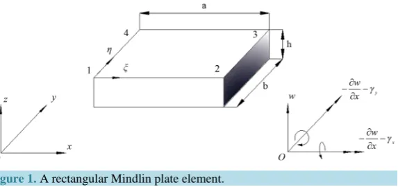
A rectangular Mindlin plate element considered in this paper is shown as Figure 1. The following is the crucial step of constructing basic full node shape functions in formulation of the multi-resolution locking-free rectangu-lar Mindlin plate element.
The displacement of a classical rectangular Mindlin plate element shown in Figure 1 can be easily acquired and concisely expressed in terms of natural coordinates as follows [16]:
(
)
(
)
4
1 4
0
1 4
0
1
b b b
i i xi xi xi yi yi yi i
x i xi i y i yi
i
w N w bN aN
N
N
θ γ θ γ
γ γ
γ γ
=
=
=
= + + + +
=
=
∑
∑
∑
Figure 1. A rectangular Mindlin plate element.
where w, γ γx, y are the transverse displacement and the shear angles around the x, y axis directions at an
arbi-trary point of the element respectively. wi, θxi, θyi, γxi, γyi are the transverse, the rotational displacements and the shear angles at node i of the element respectively. 0
i N , b
i N , b
xi
N , Nbyi are the conventional shape
functions at the node i.
The conventional shape functions 0
i N , b
i N , b
xi
N , Nbyi are defined on the domain of
[ ]
2
0,1 as follows
(
)(
)
(
)
(
)
0 1 0 2 0 3 0 4 1 1 1 1 N N N N ξ η ξ η ξη ξ η = − − = − = = − (2)(
) (
)(
)
(
)
(
)
(
)
(
)
(
)
(
)
(
)
(
)
(
)
2 2 1 2 2 2 2 2 3 2 2 4, 1 1 2 2 1
, 1 3 2 2
, 3 3 2 2 1
, 1 3 2 2
b b b b N N N N
ξ η ξ η ξ η ξ η
ξ η ξ η ξ η ξ η
ξ η ξη ξ η ξ η
ξ η η ξ ξ η ξ η
= − − + − − + = − + − − = + − − − = − + − − (3)
(
)
(
) (
)
(
)
(
)
(
)
(
)
(
)
(
)(
)
2 1 2 2 2 3 2 4, 1 1
, 1
, 1
, 1 1
b x b x b x b x N N N N
ξ η η η ξ
ξ η η η ξ
ξ η η η ξ
ξ η η η ξ
= − − = − = − − = − − − (4)
(
)
(
) (
)
(
)
(
)(
)
(
)
(
)
(
)
(
)
2 1 2 2 2 3 2 4, 1 1
, 1 1
, 1 , 1 b y b y b y b y N N N N
ξ η ξ ξ η
ξ η ξ ξ η
ξ η ξ ξ η
ξ η ξ ξ η
= − − = − − − = − − = − (5)
in which x, y.
a b
ξ = η=
Meanwhile, the shear angle γxi, γyi at node i can be read respectively as [14]:
(
) (
) (
)
(
) (
) (
)
(
) (
) (
)
(
) (
) (
)
1 2 1 4 1 4
2 2 2 3 2 3
3 2 2 3 2 3
4 2 1 4 1 4
2 2 2 2
x x x
x x x
x x x
x x x
b w w b
b w w b
b w w b
b w w b
γ δ θ θ
γ δ θ θ
γ δ θ θ
γ δ θ θ
(
) (
)
(
)
(
) (
)
(
)
(
) (
)
(
)
(
) (
)
(
)
1 1 2 1 1 2
2 1 2 1 1 2
3 1 3 4 3 4
4 1 3 4 3 4
2
2
2
2
y y y
y y y
y y y
y y y
a w w a
a w w a
a w w a
a w w a
γ δ θ θ
γ δ θ θ
γ δ θ θ
γ δ θ θ
= − − + = − − + = − − + = − − + (7)
in which the parameters
( )
(
) ( )
( )
(
) ( )
2 2
1 2, 2 2
5 6 1 2 5 6 1 2
h a h b
h a h b
δ δ
µ µ
= =
− + − + , h is denoted as the thickness
of the plate, µ as the Poisson’s ratio.
Hence, substituting (6), (7) into (1), the following equations can be obtained as:
4 1 4 1 4 1 4 1 x x y y b s
b b b
b i i xi xi yi yi
i
s s s
s i i xi xi yi yi
i
x i i xi xi
i
y i i yi yi
i
w w w
w N w bN aN
w N w bN aN
N w bN
N w aN
γ γ γ γ θ θ θ θ γ θ γ θ = = = = = + = + + = + + = + = +
∑
∑
∑
∑
(8)where w wb, s are the transverse displacement fields caused by the bending and the shear deformations
respec-tively.
In addition, there exists the following relationship
,
x x y y
w w
y x
θ =∂ −γ θ = −∂ −γ
∂ ∂ . (9)
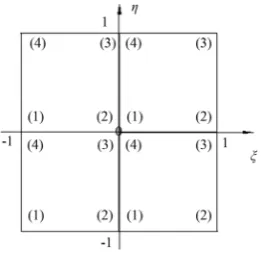
As to the proposed element, the various shape functions, regarding to a node at the point coordinate of (0, 0) as shown in Figure 2 initially defined on the domain of [0, 1]2 or viewed as for a 1/4 split node, should be ex-tended to the domain of
[
−1,1]
2 for a full node by means of shifting the element around the node (1) vertically, horizontally and obliquely respectively to the other three quadrants, thus covering the eight nodes adjacent to the basic node as displayed in Figure 3, finally the basic shape functions for the full node at the point coordinate of (0, 0) can be defined as follows:(
)
(
)
[ ]
[ ]
(
)
[
]
[ ]
(
)
[
]
[
]
(
)
[ ]
[
]
[
]
[
]
1 2 1 3 4, 0,1 , 0,1
1 , 1, 0 , 0,1
, : 1 ,1 1, 0 , 1, 0
,1 0,1 , 1, 0
0 1,1 , 1,1
I I I I I N N N N
ξ η ξ η
ξ η ξ η
φ ξ η ξ η ξ η
ξ η ξ η
ξ η ∈ ∈ + ∈ − ∈ = + + ∈ − ∈ − + ∈ ∈ − ∉ − ∉ − (10)
(
)
(
)
[ ]
[ ]
(
)
[
]
[ ]
(
)
[
]
[
]
(
)
[ ]
[
]
[
]
[
]
1 2 2 3 4, 0,1 , 0,1
1 , 1, 0 , 0,1
, : 1 ,1 1, 0 , 1, 0
,1 0,1 , 1, 0
0 1,1 , 1,1
I x I x I I x I x N N N N
ξ η ξ η
ξ η ξ η
φ ξ η ξ η ξ η
ξ η ξ η
Figure 2. The shape function domain for a 1/4 split node in a rectangular Mindlin plate.
Figure 3. The extended shape function domain for the full node at the point coordinate of (0, 0).
(
)
(
)
[ ]
[ ]
(
)
[
]
[ ]
(
)
[
]
[
]
(
)
[ ]
[
]
[
]
[
]
1
2
3 3
4
, 0,1 , 0,1
1 , 1, 0 , 0,1
, : 1 ,1 1, 0 , 1, 0
,1 0,1 , 0, 1
0 1,1 , 1,1
I y
I y
I I
y
I y N
N
N
N
ξ η ξ η
ξ η ξ η
φ ξ η ξ η ξ η
ξ η ξ η
ξ η
∈ ∈
+ ∈ − ∈
= + + ∈ − ∈ −
+ ∈ ∈ −
∉ − ∉ −
(12)
where the superscript I be denoted as b, s, γx and γy respectively.
The Kronecker delta property holds for the basic full node shape functions 1
( )
,b
φ ξ η
, 2( )
,b
φ ξ η
, 3( )
,b
φ ξ η
:( )
(
)
( )
( )
(
)
(
)
( )
(
)
( )
( )
(
)
(
)
( )
(
)
( )
( )
(
)
1
1 1
1 1 1
2
2 2
2 2 2
3
3 3
3 3 3
0, 0
0, 0 1 8 0 0
0, 0 8 8
0 0 0
0, 0
0, 0 0 8 0 0
0, 0 8 8
1 0 0
0, 0
0, 0 0 8 0 1
0, 0 8 8
0 0
b
b b
b b b
b
b b
b b b
b
b b
b b b
nodes
nodes nodes
nodes
nodes nodes
nodes
nodes n
φ
φ φ
ξ
φ φ φ
η ξ η
φ
φ φ
ξ
φ φ φ
η η ξ
φ
φ φ
ξ
φ φ φ
η ξ
∂
= = =
∂
∂ ∂ ∂
= = =
∂ ∂ ∂
∂
= = =
∂
∂ ∂ ∂
= = =
∂ ∂ ∂
∂
= = = −
∂
∂ ∂ ∂
= =
∂ ∂
(
)
0. odes η
=
∂
(13)
The basic full node shape functions
φ ξ η
1b( )
,,
φ ξ η
2b( )
,and
φ ξ η
3b( )
, [image:5.595.196.483.508.695.2]3. Displacement Subspace Sequence
In order to carry out a MRA of a rectangular Mindlin plate structure, the mutual nesting displacement subspace sequence for a rectangular Mindlin plate element should be established. In this paper, a totally new technique is proposed to construct the MRA which is based on the concept that a subspace sequence (multi-resolution sub-spaces) can be formulated by subspace basis function vectors at different resolution levels whose elements- scaling function vector can be constructed by scaling and shifting on the domain
[ ]
0,1 of the basic full node 2 shape functions. As a result, the displacement subspace basis function vector at an arbitrary resolution level (RL) of(
m+ ×1) (
n+1)
for a rectangular Mindlin plate element with the domain of a b× is formulated as follows:,00 , ,
,00 , ,
mn mn mn rs mn mn
mn mn
mn mn mn mn rs mn mn
= = =
Ψ Φ Φ Φ
Ψ Π
Ω Ω ω ω ω (14)
where , 1b , 1s ,
(
2b , 2s ,)
(
3b , 3s ,)
mn rs =φmn rs+φmn rs ley φmn rs+φmn rs lex φmn rs+φmn rs
Φ ,
, 1 , 2 ,
,
, 1 , 3 ,
0 0
x x x
y y y
mn rs mn rs ey mn rs mn rs
mn rs mn rs ex mn rs
l
l
γ γ γ
γ γ γ
φ φ φ φ = = ω ω
ω are the scaling basis function vectors,
(
)
1 , 1 ,
I I
mn rs m r n s
φ
=φ
ξ
−η
− , 2I , 2I(
,)
mn rs m r n s
φ
=φ
ξ
−η
− , 3I , 3I(
,)
mn rs m r n s
φ
=φ
ξ
−η
− , m, n denoted as theposi-tive integers, that are the scaling parameters in ξ, η directions respectively. r, s as the positive integers, the
node position parameters, that is r=0,1, 2, 3,,m, s=0,1, 2, 3,,n. lex a m
= , ley b n = ,
(
)
(
) (
)
2 1 25 6 1 2
m mh a mh a δ µ = − + ,
(
)
(
) (
)
22 2.
5 6 1 2
n nh b nh b δ µ = − +
Here,
(
mξ−r)
∈ −[
1,1]
,(
nη− ∈ −s)
[
1,1]
, ξ∈[ ]
0,1, η∈[ ]
0,1 .It is seen from Equation (14) that the nodes for the scaling process are equally spaced on the element domain of
[ ]
0,1 with a step size of 1/2 m in ξ and 1/n in η directions respectively.Scaling of the basic full node shape functions on the domain of [−1, 1]2 (precisely on the domain of
1 1 1 1
, ,
m m n n
− × −
) and then shifting to other nodes ,
r s m n
on the element domain of [0, 1]
2 will produce
the various node shape functions that are shown in the Figure 5 at the RL of 2 × 2, 3 × 3.
Since the elements in the basis functions are linearly independent with the various scaling and the different shifting parameters, the subspaces in the subspace sequence can be established and are mutually nested, thus formulating a MRA framework, that is
{
}
( ) ( ) ( )( )
11
1 1 1 1
: : ,
mn ij mn ij ij
ij i j ij i j ij i j
V V V
V span i j Z
V V + V V + V V+ +
= = ∈ ⊂ ⊂ ⊂
W
Π (15)
where Z denoted as the positive integers, Vij as displacement subspace at the resolution level of
(
i+ ×1) (
j+1)
.(a) 1( ),
b
φ ξ η (b) 2( , )
b
φ ξ η (c) 3( ),
[image:6.595.97.536.579.701.2]b φ ξ η
Figure 4. The basic full node shape functions φ ξ η1b
(
,)
, φ ξ η2b
(
,)
, φ ξ η3b
(
,)
on the domain of [−1, 1] × [−1, 1].
-1 -0.5 0
(a) 1( , )
b
φ ξ η (RL = 2 × 2) (b) 2( , )
b
φ ξ η (RL = 2 × 2) (c) 3( , )
b
φ ξ η (RL = 2 × 2)
(d) 1( , )
b
φ ξ η (RL = 3 × 3) (e) 2( , )
b
φ ξ η (RL = 3 × 3) (f) 3( , )
b
φ ξ η (RL = 3 × 3)
Figure 5. The scaled and shifted version of the basic full node shape functions φ ξ η1b
(
,)
, φ ξ η2b
(
,)
, φ ξ η3b
(
,)
on the element domain of [0, 1] × [0, 1].Thus, it can be seen that the mutually nesting displacement subspace sequence Wmn can be taken as a simple, clear and solid mathematical foundation for the MRA framework.
Based on the MRA, the deflection of a rectangular Mindlin plate element in the displacement subspace at the RL of
(
m+ ×1) (
n+1)
can be defined as followsmn
mn e
mn xmn mn
mn ymn
w γ γ
= =
d Ψ a
Ω (16)
where
T
00, 00, 00 , , , ,
e
mn= w
θ
xθ
y wrsθ θ
xrs yrs wmnθ
xmnθ
ymna , wrs,θ θxrs, yrs are the transverse,
rotational displacements respectively at the element node r ,s m n
.
It can be seen that the proposed multi-resolution element is a meshfree one whose nodes are uniformly scat-tered at each coordinate respectively, node number and position fully determined by the RL. When the RL = 2 × 2, that is a traditional 4-node rectangular Mindlin plate element, Equation (16) will be reduced to Equation (1). Hence, the traditional 4-node rectangular Mindlin plate element can be regarded as a mono-resolution one and also a special case of the multi-resolution rectangular Mindlin plate element.
4. Multiresolution Rectangular Mindlin Plate Element Formulation
According to the classical assumption of a Mindlin plate theory, the generalized function of potential energy in a displacement subspace at the resolution level of
(
m+ ×1) (
n+1)
for a rectangular Mindlin plate element with the domain of a b× can be listed as:( )
T T0 0 0 0
0 0
1 1
d d d d
2 2
d d
a b a b
p mn mn b mn mn s mn a b
mn i mni i
V x y x y
qw x y Q w
Π = +
− −
∫ ∫
∫ ∫
∑
∫ ∫
D D
κ κ γ γ
(17)
0 0.2
0.4 0.6
0.8 1
0 0.5 1 0 0.5 1
0 0.5
1
0 0.5 1 -0.2 0 0.2
0 0.5
0 0.5 1 -0.2 0 0.2
0.2 0.4
0.6 0.8
1
0.2 0.4 0.6 0.8 1 0 0.5 1
0 0.5
1
0 0.5 1 -0.2 0 0.2
0 0.5
1
[image:7.595.119.510.90.342.2]where 2 2 2 2 2 2 mn xmn ymn mn mn ymn mn xmn w x x w y y w
x y y x
γ γ γ γ ∂ ∂ − ∂ ∂ ∂ ∂ = − − ∂ ∂ ∂ ∂ ∂ − + − ∂ ∂ ∂ ∂
κ , mn xmn
ymn
γ
γ
= γ
,(
)
1 0 1 00 0 1 2
b Cb µ µ µ = − D ,
(
)
(
)
1 2 0
0 1 2
s Cs µ µ − = −
D , Cb=Eh3 12 1
(
−µ2)
, Cs =kGh=5Eh12 1(
+µ)
.E is the material Young modulus, h the thickness of the element, µ the Poisson’s ratio, q distributed transverse loadings, Qi the lump transverse loadings.
00
00
, , , ,
, , , ,
b b b e mn rs mn mn
s s s e mn rs mn mn
= =
B B B a
B B B a
κ
γ (18)
T
2 2 2
, , , , , , ,
2 2 2
y y
x x
mn rs mn rs mn rs mn rs mn rs mn rs mn rs b
rs
x y x y y x
x y γ γ γ γ ∂ ∂ ∂ ∂ ∂ ∂ ∂ = − − − − + ∂ ∂ ∂ ∂ ∂ ∂ ∂ ∂
B Φ ω Φ ω Φ ω ω ,
T
, ,
y x
s
rs mn rs mn rs γ γ
=
B ω ω .
Substitute Equation (16) into Equation (17), the concise expression can be obtained after reassembling as fol-lows:
( )
1 T T T2
e e e e e e e p Vmn mn mn mn mn mn mn mn
Π = a K a −a f −a F (19)
where e
mn
K is the element stiffness matrix, e mn
f the element distributed loading column vector, e mn
F the ele-ment lump loading column vector.
According to the potential energy minimization principle, let δΠp
( )
Vmn =0, the plate element equilibrium equations can be obtained as follows,e e e e
mn mn= mn+ mn
K a f F . (20)
The element expressions of the stiffness matrix e
mn
K , and the loading column vectors e
mn
f , e
mn
F can be
given as follows:
00 00 00
00
00
00
rs mn
e rs rs rs
mn rs ij
mn mn mn
rs mn =
k k k
K k k k
k k k
(21)
where the superscript denoted as the row number of the matrix and the subscript as the aligned element node numbering (r, s). In terms of the properties of the full node shape functions, we have
, 1 1
, 0, when 1, 1
rs
rs cd rs c r d s rs
rs cd rs c r d s
− ≤ − ≤
=
= = − > − >
∑
k k
k k
(22)
T 1 1
, 0 0
0
d d 0
b
b s b s
cd rs cd cd rs rs
s
ab ξ η
=
∫ ∫
Dk B B B B
D (23)
(
)
1 1 T
, 0 0 ,
T
, ,
d d
,
er
mn rs mn rs
er
mn rs mn rs i i i
i
a b q
m r n s Q
ξ η
ξ η
= ⋅
= − −
∫ ∫
∑
f
F
Φ
Φ (24)
where ξi, ηi is the local coordinate at the locations the lump loading acting on.
5. Transformation Matrix
In order to carry out structural analysis, the element stiffness and mass matrices e mn
K the loading column
vec-tors e
mn
f , e
mn
F should be transformed from the element local coordinate system (xyz) to the structural global coordinate system (XYZ). The transforming relations from the local to the global are defined as follows:
T
i e e e
mn= mn mn mn
K T K T (25)
T
i e e
mn = mnl mn
f T f (26)
T
i e e
mn = mnl mn
F T F (27)
where i
mn
K is the element stiffness matrix, i mn
f , i
mn
F the element loading column vectors under the global
coordinate system. e mn
T is the element transformation matrix defined as follows;
11
e
mn ij
mn
=
T
0
0
λ
λ
λ
,
cos 0 0
0 cos cos
0 cos cos
zZ
ij xX xY
yX yY
θ
θ θ
θ θ
=
λ
where θ is the intersection angle between the local and the global coordinate axes.
The structural global stiffness, mass matrix Kmn, the global loading column vectors fmn, Fmn can be ob-tained by splicing.
6. Numerical Example and Discussion
Example 1. A simply supported square plate with the geometric configuration of length L, the thickness h, the Poisson’s ratio µ and subjected to the uniform loading q. Evaluate the deflections at the center point of the plate.
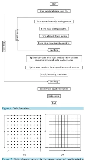
The displacement responses are found by the proposed element model (multiresolution element model) whose code flow is shown in Figure 6, the corresponding traditional 4-node locking-free Mindlin plate element model (monoresolution element model) displayed in Figure 7(a), Figure 7(b), and the wavelet element based on
two-dimensional tensor product B-spline wavelet on the interval (BSWI) [2] respectively. The BSWI is chosen
because it is the best one among all existing wavelets in approximation of numerical calculation [17] and direct-ly constructed by the tensor product of the wavelets expansions at each coordinate. The central deflections of the plate with the different thickness length ratios under the boundary conditions of four-side simply supported and four-side clamped are summarized in Table 1. One proposed element with the RL of 11 × 11 is adopted and the 4-node conventional Mindlin rectangular plate element under the corresponding meshes of 10 × 10 is also em-ployed.
Figure 6. Code flow chart.
(a) (b)
Figure 7. Finite element models for the square plate. (a) multiresolution element model (an integrated model by RL). (b) monoresolution element model (adiscretized model by mesh).
[image:10.595.167.461.79.626.2]Table 1. The deflection (w/qL/100Cb) at the center point of the simply-supported plate.
Four-side simply supported Four-side clamped
h/L Analytic Paper BSWI23 BSWI43 Analytic Paper BSWI23 BSWI43
10−3 0.4062 0.4105 1.84E−4 0.4010 0.1265 0.1290 3.8E−5 0.1115
10−2 0.4062 0.4106 0.0173 0.4067 0.1265 0.1293 0.0037 0.1269
10−1 0.4273 0.4304 0.3510 0.4273 0.1499 0.1522 0.1152 0.1505
0.15 0.4536 0.4566 0.4152 0.4536 0.1798 0.1802 0.1592 0.1788
0.20 0.4906 0.4933 0.4678 0.4904 0.2167 0.2183 0.2047 0.2172
0.30 0.5956 0.5968 0.5861 0.5957 0.3227 0.3235 0.3187 0.3246
0.35 0.6641 0.6631 0.6579 0.6641 0.3951 0.3902 0.3898 0.3937
than the meshing and the re-meshing to modulate element node number for the following two reasons. Firstly, the RLis based on the MRA framework which is constructed on a rigorous mathematical basis and the full node shape functions result in an integrated model, while the mesh, which resorts to the empiricism and the split node shape functions lead to a discretized model, has no MRA framework. Secondly, the stiffness matrix and the loading column vectors of the proposed element can be obtained automatically around the nodes while those of the traditional 4-node rectangular plate elements acquired by the artificially complex reassembling around the elements. It can be seen that the computational accuracy and efficiency of the proposed element model is higher than the other two.
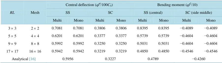
Example 2. Two square plates are subjected to the uniform loading q with the geometric configuration of length L, thickness h, Poisson’s ratio µ and the ratios of L/h = 10−3 and L/h = 0.3 respectively. Evaluate the deflections and moments at the center point of two plates under such boundary conditions as four sides simply supported or clamped.
The displacement responses and moments are evaluated by the proposed multiresolution element method, the traditional monoresolution element method. The central deflections and the bending moments for a thin and at hick plate with the boundary conditions as simply supported four edges (SS) and the clamped four edges (SC) under the different RLs and meshes are displayed respectively in Table 2 and Table 3. The RL of the proposed and the corresponding meshes of the conventional are compared. It can be seen that the analysis accuracies with the proposed and the conventional are gradually improved respectively with the RL reaching high and the mesh approaching dense. However, the RL adjusting is more rationally and efficiently to be implemented than the meshing and remeshing to modulate element node number because the RL adjusting is based on the MRA framework which is constructed on a rigorous mathematical basis while the meshing or remeshing, which re-sorts to the empiricism, has no MRA framework. Thus, the computational efficiency of the proposed element method is higher than the traditional one. In this way, the proposed element exhibits its strong capability of ac-curacy adjustment and its high power of resolution to identify details (nodes) of deformed structure by means of modulating its resolution level, just as a multi-resolution camera with a pixel in its taken photo as a node in the proposed element. There appears no mesh in the proposed element just as no grid in the image. Hence, an ele-ment of superior analysis accuracy surely has more nodes when compared with that of the inferior just as a clearer photo contains more pixels.
Table 2. The deflection for thin plate (h/L = 10−3) under different RLs and meshes.
RL Mesh
Central deflection (ql4/100C
b) Bending moment (ql2/10)
SS SC SS (central) SC (side middle)
Multi Mono Multi Mono Multi Mono Multi Mono
3 × 3 2 × 2 0.5063 0.5063 0.1480 0.1480 0.6602 0.6602 −0.3551 −0.3551 5 × 5 4 × 4 0.4328 0.4328 0.1403 0.1403 0.5217 0.5217 −0.4761 −0.4761 9 × 9 8 × 8 0.4129 0.4129 0.1304 0.1304 0.4892 0.4892 −0.5028 −0.5028 17 × 17 16 × 16 0.4079 0.4079 0.1275 0.1275 0.4814 0.4814 −0.5104 −0.5104
Analytical [16] 0.4062 0.1265 0.4789 −0.5133
Table 3. The deflection for thick plate (h/L = 0.3) under different RLs and meshes.
RL Mesh
Central deflection (ql4/100C
b) Bending moment (ql2/10)
SS SC SS (central) SC (side middle)
Multi Mono Multi Mono Multi Mono Multi Mono
3 × 3 2 × 2 0.7081 0.7081 0.3806 0.3806 0.8395 0.8395 −0.4089 −0.4089 5 × 5 4 × 4 0.6201 0.6201 0.3377 0.3377 0.5739 0.5739 −0.4604 −0.4604 9 × 9 8 × 8 0.5992 0.5992 0.3250 0.3250 0.5031 0.5031 −0.4604 −0.4604 17 × 17 16 × 16 0.5942 0.5942 0.3219 0.3219 0.4850 0.4850 −0.4546 −0.4546
Analytical [16] 0.5956 0.3227 0.4789 −0.4260
proposed method. Moreover, since the multiresolution rectangular Mindlin plate element model of a structure usually contains much less elements than the traditional element model, thus requiring much less times of trans-formation matrix multiplying, the computation efficiency of the proposed method appears much higher than the traditional in the step of element matrix transformation. In addition, because of the simplicity and clarity of a full node shape function formulation with the Kronecker delta property and the solid mathematical basis for the new MRA framework, the proposed method is also superior to other corresponding MRA methods in terms of the computational efficiency, the application flexibility and extent. Hence, taking all those causes into account, the conclusion can be drawn that the multi-resolution Mindlin rectangular plate element method is more ration-ally, easily and efficiently to be executed, when compared with the traditional 4-node Mindlin rectangular plate element method or other corresponding MRA methods, and the proposed element would be the most accurate one formulated ever since.
[image:12.595.85.537.255.385.2]7. Conclusion and Prospective
A new multiresolution finite element method that has both high power of resolution and strong flexibility of analysis accuracy is introduced into the field of numerical analysis. The method possesses such prominent fea-tures as follows:
• A novel technique is proposed to construct the simple and clear basic full node shape function for a lock-ing-free Mindlin rectangular plate element, which unveils the secret behind assembling artificially of node-related items in global matrix formation by the conventional FEM.
• A mathematical basis for the MRA framework that is the mutually nesting displacement subspace sequence, is constituted out of the scaled and shifted version of the basic full node shape function, which brings about the rational MRA concept together with the RL.
• The traditional 4-node Mindlin rectangular plate element and method is a monoresolution one and also a special case of the proposed. An element of superior analysis clarity surely contains more nodes when com-pared with that of the inferior.
• The RL adjusting for the multiresolution Mindlinplate element model is laid on the rigorous mathematical basis while the meshing or remeshing for the monoresolution is based on the empiricism. The proposed element method can consolidate all corresponding irrational MRA approaches. Thus, the accuracy of a plate structural analysis is replaced by the clarity, the irrational MRA by the rational and the mesh by the RL that is the discretized model by the integrated.
• A quite new concept is introduced into the FEM that the structural analysis clarity is actually determined by the RL—the density of node uniform distribution, not by the mesh.
• With advent of the new finite element method [18]-[20], the rational MRA will find a wide application in numerical solution of engineering problems in a real sense.
The upcoming work will be focused on the treatment of interface between multiresolution elements of differ-ent RL. The interface may be extended to the bridging domain in which a transitional elemdiffer-ent can be used just as PS images of different RL. The transitional element could also be constructed by the technique of scaling and shifting of the basic full node shape function to virtual or real nodes.
References
[1] Zienkiewicz, O.C. and Taylor, R.L. (2006) The Finite Element Method. 6th Edition, Butterworth-Heihemann, London. [2] Xiang, J.W., Chen, X.F., He, Y.M. and He, Z.J. (2006) The Construction of Plane Elastomechanics and Mindlin Plate
Elements of B-Spline Wavelet on the Interval. Finite Elements in Analysis and Design, 42, 1269-1280. http://dx.doi.org/10.1016/j.finel.2006.06.006
[3] He, Z.J., Chen, X.F. and Li, B. (2006) Theory and Engineering Application of Wavelet Finite Element Method. Science Press, Beijing
[4] Yu, Y., Lin, Q.Y. and Yang, C. (2013) A 3D Shell-Like Approach Using Element-Free Galerkin Method for Analysis of Thin and Thick Plate Structures. Acta Mechanica Sinica, 29, 85-98. http://dx.doi.org/10.1007/s10409-012-0159-7 [5] Chen, L., Cheng, Y.M. and Ma, H.P. (2015) The Complex Variable Reproducing Kernel Particle Method for the
Anal-ysis of Kirchhoff Plates. Computational Mechanics, 55, 591-602. http://dx.doi.org/10.1007/s00466-015-1125-6 [6] Rad, M.H.G., Shahabian, F. and Hosseini, S.M. (2015) A Meshless Local Petrov-Galerkin Method for Nonlinear
Dy-namic Analyses of Hyper-Elastic FG Thick Hollow Cylinder with Rayleigh Damping. Acta Mechanica, 226, 1497- 1513. http://dx.doi.org/10.1007/s00707-014-1266-2
[7] Liu, H.S. and Fu, M.W. (2013) Adaptive Reproducing Kernel Particle Method Using Gradient Indicator for Elas-to-Plastic Deformation. Engineering Analysis with Boundary Elements, 37, 280-292.
http://dx.doi.org/10.1016/j.enganabound.2012.09.008
[8] Sukumar, N., Moran, B. and Belytschko, T. (1998) The Natural Elements Method in Solid Mechanics. International Journal of Numerical Methods in Engineering, 43, 839-887.
http://dx.doi.org/10.1002/(SICI)1097-0207(19981115)43:5<839::AID-NME423>3.0.CO;2-R
[9] Sukumar, N., Moran, B. and Semenov, A.Y. (2001) Natural Neighbor Galerkin Methods. International Journal of Nu-merical Methods in Engineering, 50, 1-27.
http://dx.doi.org/10.1002/1097-0207(20010110)50:1<1::AID-NME14>3.0.CO;2-P
196, 1827-1846. http://dx.doi.org/10.1016/j.cma.2006.10.002
[11] Feng, X.T. and Yang, C.X. (2001) Genetic Evolution of Nonlinear Material Constitutive Models. Computer Methods in Applied Mechanics and Engineering, 190,5957-5973. http://dx.doi.org/10.1016/S0045-7825(01)00207-9
[12] Jäger, P., Steinmann, P. and Kuhl, E. (2006) Modeling Three-Dimensional Crack Propagation—A Comparison of Crack Path Tracking Strategies. International Journal of Numerical Methods in Engineering, 66, 911-948.
[13] Fagerström, M. and Larsson, R. (2006) Theory and Numerics for Finite Deformation Fracture Modelling Using Strong Discontinuities. International Journal of Numerical Methods in Engineering, 76, 1328-1352.
http://dx.doi.org/10.1002/nme.1573
[14] Luccioni, B.M., Ambrosini, R.D. and Danesi, R.F. (2004) Analysis of Building Collapse under Blast Loads. Engineer-ing Structure, 26, 63-71. http://dx.doi.org/10.1016/j.engstruct.2003.08.011
[15] Wang, Z.Q., Lu, Y. and Hao, H. (2004) Numerical Investigation of Effects of Water Saturation on Blast Wave Propa-gation in Soil Mass. ASCE-Engineering Mechanics, 130, 551-561.
http://dx.doi.org/10.1061/(ASCE)0733-9399(2004)130:5(551)
[16] Long, Y.Q., Cen, S. and Long, Z.F. (2009) Advanced Finite Element Method in Structural Engineering. Springer- Verlag, Berlin, Heidelberg; Tsinghua University Press, Beijing. http://dx.doi.org/10.1007/978-3-642-00316-5
[17] Cohen, A. (2003) Numerical Analysis of Wavelet Method. Elsevier Press, Amsterdam, Holland.
[18] Xia, Y.M., Liu, Y.X., Chen, S.L. and Tan, G. (2014) A Rectangular Shell Element Formulation with a New Multireso-lution Analysis. Acta Mechanica Solida Sinca, 27, 612-625. http://dx.doi.org/10.1016/S0894-9166(15)60006-4 [19] Xia, Y.M. (2014) A Multiresolution Finite Element Method Based on a New Quadrilateral Plate Element. Journal of
Coupled Systems and Multiscale Dynamics, 2, 52-61. http://dx.doi.org/10.1166/jcsmd.2014.1040
[20] Xia, Y.M. and Chen, S.L. (2015) A Hexahedron Element Formulation with a New Multi-Resolution Analysis. Science China (Physics, Astronomy and Mechanics), 58, Article ID: 014601-10. http://dx.doi.org/10.1007/s11433-014-5425-1
![Figure 4. The basic full node shape functions φ()1bξ η, , φ()2bξ η, , φ()3bξ η, on the domain of [−1, 1] × [−1, 1]](https://thumb-us.123doks.com/thumbv2/123dok_us/7911058.745626/6.595.97.536.579.701/figure-basic-node-shape-functions-bx-bx-domain.webp)
![Figure 5. The scaled and shifted version of the basic full node shape functions φ()1bξ η, , φ()2bξ η, , φ()3bξ η, on the element domain of [0, 1] × [0, 1]](https://thumb-us.123doks.com/thumbv2/123dok_us/7911058.745626/7.595.119.510.90.342/figure-scaled-shifted-version-basic-functions-element-domain.webp)