Munich Personal RePEc Archive
Decision Making Using Rating Systems:
When Scale Meets Binary
Bargagliotti, Anna E. and Li, Lingfang (Ivy)
University of Memphis, Shanghai University of Finance and
Economics
25 August 2009
Online at
https://mpra.ub.uni-muenchen.de/16969/
Decision Making Using Rating Systems: When Scale Meets Binary
Anna E. Bargagliotti Lingfang (Ivy) Li
Department of Mathematical Sciences School of Economics
University of Memphis Shanghai University of Finance and Economics
[email protected] [email protected]
August 27, 2009
Abstract
Rating systems measuring quality of products and services (i.e., the state of the world) are widely used to solve the asymmetric information problem in markets. Decision makers typically makebinarydecisions such as buy/hold/sell based on aggregated individuals’ opinions presented in the form of ratings. Problems arise, however, when different rating metrics and aggregation procedures translate the same underlying popular opinion to different conclusions about the true state of the world. This paper investigates the inconsistency problem by examining the mathematical structure of the metrics and their relationship to the aggregation rules. It is shown that at the individual level, the onlyscale metric (1,. . . ,N) that reports people’s opinion equivalently in the a binary metric (-1, 0, 1) is one where N is odd and N-1 is not divisible by 4. At aggregation level, however, the inconsistencies persist regardless of which scale metric is used. In addition, this paper provides simple tools to determine whether the binary and scale rating systems report the same information at individual level, as well as when the systems differ at the aggregation level. 1 2
1JEL: D82, D70. Keywords: rating, ranking, preference, asymmetric information. 2
1
Introduction
Rating systems are widely used in business, political systems, and in our daily lives as methods
of containing and communicating information that is crucial to the decision making process. For
instance, investors make decisions by consulting ratings of financial products, online shoppers
com-pare products by examining seller and product ratings, doctors make diagnoses based on a patient’s
rating of their well-being, students refer to university rankings to decide which school to attend,
and universities use rating systems to monitor professors’ performance in teaching. Rating systems
provide a way to summarize public opinion in an organized manner. A rating system is defined
by a rating metric and an aggregation rule that combines individual’s ratings into a single overall
score. Several forms of rating systems exist. Two popular systems are thebinary system and the
scale system. For example, eBay’s reputation system asks users to rate a buyer or seller in a binary
rating system {−1,0,1}, where −1 is considered a negative rating, 0 is a neutral rating, and 1
is a positive rating. On the other hand, Amazon.com asks raters to use a scale rating system of
{1,2,3,4,5}where one is considered worst and five is best3. Using information about the aggregate
of individuals’ opinions in either the scale or the binary system, a decision maker is required to
draw a conclusion about a product or a service. Typically, this conclusion has a binary outcome
such as buying, holding, or selling of a stock. Problems and paradoxes arise, however, when the
scale rating system leads a decision maker to make one decision but the binary rating system leads
the decision maker to a contradictory decision.
To illustrate how the aggregated information from the scale ratings can be contradictory to that
of the binary ratings, consider two groups of ten financial analysts rating a stock in both a scale
system and a binary system. Using a scale of one to five (strong buy = 5, buy = 4, hold = 3, under
perform = 2, and sell = 1), half the analysts in the first group rate the stock as a 4 and the other
half rate it as a 2. In a binary system (buy = 1, hold = 0, and sell = -1), the group’s collective
decision is to “buy” the stock. The second group of ten analysts all rate the stock 3 in the scale
system and aggregate to “hold” in the binary system. The scale ratings of both groups suggest the
3
overall opinion of the stock is neutral – group one is split 50-50 around 3 and group two all rates
3. On the other hand, in the binary system, the two groups give contradictory collective decisions
– group one says “buy” while group two says “hold.”
It is hypothesized these types of inconsistencies are mainly due to human errors, such as a person
not understanding the meaning of the scale, or a person’s strategic dishonest rating. In this paper,
we illustrate that even without human errors and strategic ratings, inconsistent decision outcomes
can occur. In fact, the two metrics and aggregation procedures can translate the same underlying
popular opinion to different decision outcomes due to the restrictions placed by the mathematical
structures of the systems.
This paper investigates the inconsistency problem by examining the mathematical structure of the
metrics and their relationship to the aggregation rules. We show that at the individual rating
level, the only scale metric{1, . . . , N}that can report a person’s opinion equivalently as the binary
metric {−1,0,1} is one where N is odd and N −1 is not divisible by 4. At the aggregate level,
however, the inconsistencies persist regardless of which scale metric is used. The differences in the
aggregation systems are characterized and simple tools are illustrated to determine whether the
binary and scale rating systems are reporting the same information both at the individual rater’s
level as well as at the collective aggregate level.
2
Related Literature
Ranking systems and rating systems are two closely related methods for capturing and
summa-rizing public opinion proposed in the literature. In general, a ranking system asks participants
to rank-order alternatives while a rating system asks participants to score an alternative on an
arbitrary scale. Research on these systems has focused on obtaining best methods for capturing
and representing people’s opinions. Connections and distinctions between the two types of systems
have also been made in the literature. In both systems, the alternatives can represent the object of
ranking systems are a special case of rating systems (Droba, 1931). For example, a person may be
asked to organize alternatives into three different groups representing the worst, middle, and best.
In the case where there are numeric values associated with each category (e.g, worst = 0, middle
= 1, and best = 2), each participant ranks according to a rating. These types of ranking methods
not only provide relative comparisons among alternatives but they also provide rating information
about the alternatives.
Although rating systems are more general than ranking systems, previous work has focused
pri-marily on rankings. The problem of aggregating ranking preferences is one of the most vexing
and difficult in economics, political science, and decision science. Issues of existence of desirable
aggregation functions date back at least as far as Arrow’s Impossibility Theorem (Arrow, 1963).
Since then, numerous papers have discussed inconsistencies with voting and social choice rules used
for aggregating preferences as well as new interpretations and resolutions (Moulin, 1988, Sen, 1970,
1986, Saari, 2001a, 2001b, Li and Saari, 2008).
As with ranking systems, similar issues and inconsistencies arise when using rating systems to
capture and aggregate information as shown in the above example. Two possible explanations have
been offered as the cause of the inconsistencies. They are: (1) people misunderstand or misinterpret
the rating scale, and (2) people rate strategically.
In marketing, the debate on which scale to use began several decades ago (Lehmann and Hulbert,
1972, McDaniel and Gates, 2006). In recent years, researchers find that people do not differentiate
greatly among the scale values and assign high ratings to most items (McCarty and Shrum, 2000,
Greenleaf, Bickart, and Yorkston, 1999). Because the rating data does not capture details about
people’s opinions, it makes it difficult to use in choosing an effective marketing strategy. It is
hypothesized that this phenomena occurs because people may not understand the meaning of the
rating scale. In social science and psychology research, Alwin and Krosnick (1985) also observe
that rating methods do not differentiate well among people’s opinion because respondents tend to
rate everything high. Landy and Farr (1980) argue that the cognitive characteristics of raters seem
to explain the bias toward high ratings in rating systems. For example, changing a scale from -3
values used in the scale influence respondents’ interpretation (Schwarz et al., 1991).
Another possible explanation offered in the literature for the inconsistencies surrounding data is
strategic behavior. Cleveland and Murphy (1992) and Murphy et al. (2004) suggest that the reason
for raters giving ratings that appear psychometrically suspect is due to their different individual
goals when completing performance appraisals. For example, raters may want to maintain
har-mony within the workgroup or possibly motivate subordinates to perform better in the future.
Similar hypotheses have been explored in the economic literature focusing on strategic behavior in
information aggregation (see Carwford and Sobel, 1982, Sobel, 2006, Morgan and Stocken, 2008).
Because rating systems are a part of market reputation systems, feedback mediators are an
im-portant factor in designing and improving reputation systems (Dellarocas et al., 2006). Relying
on a user feedback system that yields poor representations of user’s opinions can lead to mistrust
and misuse of a particular market. For example, the design of eBay’s bi-lateral reputation system
leads to problems of bias towards positive ratings (See Dellarocas and Woods, 2006, Klein et al.,
2006, and Li forthcoming). In this context, understanding the mathematical structure of the rating
system can help determine a successful design for feedback ratings in a market system.
By reviewing the current literature, it can be seen that the existing explanations of the
inconsis-tencies and issues with rating systems are due to human limitations and behaviors. The focus of
this current paper is to characterize the inconsistencies that can occur among the binary and scale
rating system in terms of the mathematical structure of the systems. While previous contributions
explain the “meaning” of the scales and how people interpret them, this paper strives to understand
the structural differences among the scales. Even without human errors and strategic behavior, the
results show inconsistencies between the binary system and scale rating system persist.
3
Framework
Suppose a decision maker needs to draw a conclusion about a product, service, or trade based on
of scale and binary ratings capturing the public’s opinion about the product or service. Scale
information may offer more details about the intensity of people’s opinion while binary information
may capture a more direct up-or-down-like measure. Either could prove useful to the decision maker.
Using these two types of ratings, the decision maker can make a decisive conclusion. Typically,
this conclusion will have a binary outcome such as the decision maker deciding to buy, hold, or
sell the product; or the decision maker deciding to use, maybe use, or not use a service. Problems
arise, however, when the information conveyed through the scale ratings is not consistent with the
information conveyed through the binary rating; therefore leading the decision maker to different
conclusions depending on which rating data he/she examines.
The scale and binary rating data collected is a gathering of people’s opinions about the product,
service, or trade. For example, a committee of faculty members may be asked to give scale and
binary ratings representing their opinion of the quality of a particular job candidate. In such
instances, the product, in this example, the job candidate, being evaluated possesses an actual true
unobservable quality. This true state of the product will be denoted as T S throughout the paper.
Although there exists a T S for the product, each rater may perceive its quality differently. For
each rater, we define their perception byP S, the perceived state of the product, to represent their
individual opinion aboutT S.
When presented with a rating system, a rater must translate their P S into a rating in the given
rating metric. This rating is then what is available to the decision maker to aid in the decision
making process. When the information conveyed through the scale system is not consistent with
the information conveyed through the binary system, the decision maker may have evidence to
support different conclusions depending on which rating data he/she consults.
In order to explore this inconsistency issue, we decompose the rating procedure into two sequential
levels – the individual level and the aggregation level. At the individual level, individuals choose
a rating score in the available metric closest to their perceptionP S. At the aggregation level, the
individuals’ ratings are combined using an averaging function. At the first level, it is reasonable
to expect that individuals who express the same opinion in the scale system should express the
system then they should also agree in the binary system. At the second level, the aggregate results
from the scale and binary metrics should lead the decision maker to the same conclusions about
T S. These two desirable properties can be summarized as: (1) the representation of individual’s
opinions in the scale and binary metric must be equivalent (i.e., individuals who express the same
opinion in the scale system should express the same opinion in the binary system), and (2) the
aggregation of individuals’ opinions in each system must be consistent (i.e., lead the decision maker
to the same conclusion.) The goal of this paper is to explain these properties mathematically and
provide tools for decision makers to identify when the properties are satisfied. To do this, we begin
by formally defining a rating system.
A rating system is composed of two separate items: a metric and an aggregation rule. Individuals
rate in the metric and then aggregate their scores according to a specified rule. The metric is
typi-cally a discrete set of integers contained in an interval. For example, the scale metric{1,2,3, ...,10}
can be expressed as the set of integers in the interval [1,10]. An aggregation rule combines
peo-ple’s opinions into one overall score. Typically, the rule takes the form of an averaging function.
Mathematically, a rating system can be defined in the following manner.
Definition 1 Let int[m, n]k be the k-product of the set of integer values in the interval [m,n].
A rating system is a set { int[m,n], R } where int[m,n] is the set of integers between m and n
containing m and n. R is a function fromint[m, n]k to the interval [m,n] where k is the number of
people rating.
R: int[m, n]k →[m, n]
The binary rating system can therefore be specified as{ int[-1,1],Rb }where int[-1,1] ={-1, 0, 1 }
and Rb: int[−1,1]k →[−1,1]. The scale system can be written as { int[1,N], R
s } where int[1,N]
4
Translating Individual Rating from Scale to Binary
As described above the true state,T S, can be thought of as the true quality of a product or service
that exists outside of a decision maker’s or rater’s opinion. The true stateT S is modeled as a point
in the interval [1, N].4 Each rater may perceiveT S differently and rate the closest available integer
to their perceived state,P S, in the given metric. IfP Sis halfway between two rating options, then
without loss of generality, the rater will choose the higher integer option. 5
Example 1 Suppose two people rate a service using the metric int[1,5]. Person A perceives the
service as 2.1 and person B perceives it at 1.9. Since the available metric requires the individuals
to rate 1, 2, 3, 4, or 5, both individuals rate2. Both 2.1 and 1.9 perceived states are closest to the
integer 2.
If the same individuals rate in the binary metric, how are their opinions represented? Rating in the
binary metric requires an individual to translate their P S from the interval [1, N] to the interval
[−1,1]. The perceived state in the interval [1, N] can be translated to a point in the interval [−1,1]
using a linear transformation. Once this step is complete the individuals will again rate at the
closest available option to theirP S in the binary metric.
Definition 2 Given metrics int[a, b] and int[c, d]. Any point k ∈ [a, b] can be transformed to a
pointj ∈[c, d] by the following linear transformation:
k= da−cb d−c +
b−a
d−cj (1)
This means that a perceived state P S1 in metric 1 can be transformed into a perceived state P S2
in metric 2 by:
4
Typically, people think in a positive continuous interval thus it is natural to capture quality and perception in the positive interval [1, N]
5
For simplicity and without loss of generality, it is assumed that if an individual has perceived state half way between two integer values, then the individual will cast their rating as the highest value. For example, in a [1,10] scale metric, if a rater hasP S= 8.5, then the individual will rater= 9. If a rater has a perceived state of 1
2 in the
P S1 = dad−−cbc +bd−−acP S2 (2)
Therefore a perceived state,P S, in metric [1, N] can be transformed to a perceived state in [−1,1]
by P S[1,N]=1+2N+N−1
2 P S[−1,1].
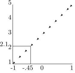
Example 2 Person A and person B have perceived states, 2.1 and 1.9 respectively. Then, person
A has perceived state equal to P S[−1,1] = (2.1− 1+52 )(5−21) = −.45 in the binary metric. This
transformation is modeled in Figure 1. Similarly, person B has perceived state equal to −.55.
Person A and B may rate −1, 0, or 1 in this metric. Since −.45 is closest to 0, A rates 0. Since
[image:10.595.209.334.377.499.2]−.55 is closest to −1, B rates −1.
Figure 1: Transforming scores between metrics
-1 0 1
1 2 3 4 5
✠ ✠
✠ ✠
✠ ✠
✠ ✠
✠ ✠✠
-.45 2.1
Examples 1 and 2 illustrate how the two metrics can represent the same opinions differently. In
the scale metric, personAandB rate the same, however, in the binary metric they rate differently.
In this situation, a decision maker examining both the scale and binary ratings is given conflicting
information. Ideally, the two metrics would represent rater’s opinions in the same manner. We
define this desired property of equivalency in the following manner:
Definition 3 A scale metric and a binary metric are called equivalent if and only if for every
4.1 Scale and Binary Equivalency
Because two metrics can represent the same underlying opinions differently, a natural question to
ask is whether there are specific conditions under which the scale and binary will be equivalent (i.e.,
rater’s opinions that are the same in the scale will also be the same in the binary). In order for
a discrepancies between the metric’s representation of people’s opinions to occur, two ratings that
round to the same integer in [1, N] must round to different integer values in [−1,1] after applying
the linear transformation. Thus, in order to ensure equivalency, the rounding points in the binary
metric must be the image of the rounding points in the scale metric under the linear transformation.
The rounding points represent the cut-off points where a rater will either round up or round down.
In the binary metric, the rounding points are −.5 and.56. Raters having aP S[−1,1] less than −.5
will rate −1, those between −.5 and .5 will rate 0, and those with P S[−1,1] larger than .5 will rate
1. In order for the scale and binary metrics to be equivalent, the pre-image of −.5 and .5 under
the linear transformation, given by 1+ 1+N
2
2 and
N+1+N
2
2 , must not be not integer values. If they are
integer values, then raters will be “split” at the rounding point leaving them to rate the same in
the scale metric but not the same in the binary metric. The following two examples highlight this
point.
Example 3 Consider the scale metric [1,5]. Under the linear transformation, the pre-image of
rounding point −.5 is the number 2. In order to create a discrepancy between the metric’s
repre-sentation of the two opinions, choose two raters who rate differently in the binary metric and are
split by rounding point in −.5. Suppose rater 1 has P S[−1,1] equal to −.4 and rater 2 has P S[−1,1]
equal to −.7. In the binary metric, these raters will not rate the same with rater 1 rating 0 and
rater 2 rating -1. When applying the inverse of the linear transformation to their opinions, we see
that rater 1 and rater 2 agree in [1,5] and both rate 2. By Definition 3, the [1,5] metric and the
binary metric are therefore not equivalent.
6Throughout this paper, we use cut-off points −1 2 and
1
2 for simplicity, however, these can be generalized to any
two points −1
s and
1
s in the interval [−1,1]. To determine the cut-off points of a particular population of raters,
Example 4 Consider the scale metric [1,7]. Under the linear transformation, the pre-image of
rounding point −.5 is 2.5. Because the pre-image is not integer valued, raters who are split by a
rounding point in the binary will also be split in the scale thus causing them not to rate the same
in [1,7]. Rater 1 and rater 2 will still rate 0 and -1 respectively in the binary metric but in [1,7],
their opinions−.4 and−.7fall on different sides of2.5leading rater 1 to rate2 and rater 2 to rate
3. In this case, the raters rate differently in both in the scale and binary metric.
In order to ensure equivalency between the two systems, two ratings that round to the same integer
in [1, N]must round to the same integer values in [−1,1] after applying the linear transformation.
The following theorem summarizes the only case for which this happens. The proof is deferred to
the Appendix.
Theorem 1 The scale system and binary system are equivalent if and only ifN is odd and N−1
is not divisible by4.
For all other N, it is possible to pick points in specific intervals that cause the scale and binary
metric to be nonequivalent. As an illustration, consider the scale metric withN odd butN−1 not
divisible by 4. In this metric, the pre-image under the linear transformation of the cut-off points
of −.5 and .5 are the integer values 1+ 1+N
2
2 and
N+1+N
2
2 respectively. Choose raters 1 and 2 such
that theirP S’s lie on either side of 1+ 1+N
2
2 but within the interval [ 1+1+N
2
2 −12, 1+1+N
2
2 +12], then the
raters will both rate at the integer value 1+ 1+N
2
2 in the scale metric but will be split in the binary
metric because theirP S’s will fall on either side of the−.5 cut-off point. Similarly, whenN is even,
one can always choose rater perceived states in such a way that they round to the same integer in
the scale metric but are split in the binary.
Therefore, Theorem 1 completely characterizes all inconsistencies among raters at the individual
level. The characterization points out how the metrics represent information differently and can
4.2 Implications of Differences between Binary and Scale Metric at the
Indi-vidual Rater Level
Except for the case where N is odd and is not divisible by 4, the binary and the scale metric
interpret ratings in a different manner. What are the implications of the differences between the
systems for these cases? Do the systems tend to penalize or inflate the ratings? In Example 1
and 2 above, person A’sP S is represented as a 0 rating in the binary system and a 2 in the scale
system. Because the 2 rating is below the neutral rating in the [1,5] scale (i.e., below the midpoint
of 3) and 0 is the neutral rating in the binary metric, the binary system actually represents A’sP S
at a higher value than the scaled. The opinion in the binary system is thus interpreted as higher
than A’s opinion in the scale. This means that with perceived state equal to 2.1 in [1,5], the binary
system actually inflates the score to 0 in [−1,1]. To the contrary, person B’s perceived state (1.9
in [1,5]) is penalized in the binary system. Person B rates -1 in the binary system that has a lower
interpretation than the 2 in the scale. The following theorem follows directly from Definition 2 to
characterize the regions of the interval [1, N] that the binary system distorts.
Theorem 2 For a fixed N, let P Ss equal a rater’s perceived state in the scale system and rs be
its equivalent rating given by rs={k : k∈ [1,N] and min|P Ss-k|}. Let xsb equal the translation of
rs into the binary system. Note that xsb may not be a rating and thus not be an integer. Let P Sb
be the translation of P Ss in the binary system and rb be it’s rating given by rb={j :j∈ [-1,1] and
min|P Sb-k|}. The penalty or benefit associated with every rating is given by rb-xsb if using the
binary system instead of the scale system.
In order to compute that amount of distortion created by the metric, the difference in what the
rating should be (i.e., the translated ranking xsb) and the actual binary rating rb) is computed.
The following example illustrates the computation.
Example 5 Suppose N = 5. Let P Ss ∈ [1.5,2] be given. Then the individual will rate rs= 2 in
the binary system. However, in the binary system, an individual with PS∈ [1.5,2] will rate rb=-1.
Therefore, rb-xsb=−0.5 penalty in the binary system.
If PS ∈ [2,2.5], the individual will rate as a rs= 2 in the scale system. As before, the rating 2 is
equivalent to the positionxsb=−0.5 in the binary system. However, for PS∈[2,2.5], the individual
will rate rb=0. Therefore,rb-xsb= 0.5 benefit in the binary system.
Theorem 3 The only scale system for which the binary systemdoes not distortpeople’s opinion
is the case where N is odd and N-1 is not divisible by 4.
The theorem follows as a direct consequence of Theorems 1 and 2. This underscores the importance
of scale selection in applications.
5
Aggregation Procedures Using Different Metrics
Once individuals have cast their ratings, the information is aggregated to form an overall score.
An aggregation rule, R, is typically defined as an average or weighted average function. Two issues
can arise when aggregating ratings: (1) the average score in the scale system may not be consistent
with the average score computed in the binary system, and (2) the decision the average score in the
scale system may lead one to make is not the same as the decision the average score in the binary
system leads one to make. These two issues may arise even when using a scale metric whereN is
odd and N −1 is not divisible by 4. Consider the following example to motivate the aggregation
discussion.
Example 6 Mike is interviewed for a job and 10 people in the office are asked to rate him on
a scale of 1-7. Among the 10 people, 4 have perceived states near 4 and 6 have perceived states
around6. In addition to rating Mike on a scale, each of the10people is asked directly whether they
would like to hire Mike, whether they would like to wait and see the next candidate, or whether they
system, the aggregated average score = 5.2(computed as (4(4) + 6(6)) /10). This score translates
to a score of .4 in the binary system which yields the decision to wait and see the next candidate
before making a decision about Mike. In the binary system,4people choose to wait and see the next
candidate while the other 6 raters choose to hire him. The aggregated average score in this system
is.6(computed as (0(4) + 1(6)) /10). According to the binary aggregation, an offer is extended to
Mike.
The example illustrates that even when using a scale whereN is odd andN−1 is not divisible by
4, the aggregated ratings may not be consistent. In addition, the decisions the aggregated scores
lead to may also be different. The following sections provide simple tools to check when these
inconsistencies occur.
5.1 Issue 1: Average Scores Are Not Consistent
In the binary system, let b1, b2, and b3 represent the number of −1,0,1 ratings respectively. In
the scale system, let s1, s2,..., sN represent the number of 1,2, ..., N ratings respectively. The
average functionRb aggregates the binary ratings as: b1b+3b−2b+1b3 and Rs aggregates the scale ratings
as:
PN i=1isi
PN
i=1si. Thus, Rb is defined as a function fromint[−1,1]
k →[−1,1] andR
s is a function from int[1, N]k →[1, N].Comparing the two average functions amounts to understanding the valuesb
1,
b2,b3 and s1,s2,...,sN must equal in order for the two rules to output consistent scores.
Definition 4 Let Rx: int[a, b]k →[a, b]andRy: int[c, d]k →[c, d]. For each of thekraters, denote
rxi and ryi as rater i′s ratings in int[a, b] and int[c, d] respectively. Then, Rx and Ry are called
consistent for the group of k raters if and only if the aggregated score in one metric is equal to
a linear transformation of the aggregated score in the other metric. i.e., Rx and Ry satisfy the
following equation:
Ry(ry1, . . . , ryk) =
bc−da b−a +
d−c
For Rx and Ry being the average function, then the equation can be written as:
1
k k
X
i=1
ryi=
bc−da b−a +
d−c b−a(
1
k k
X
i=1
rxi). (2)
Because different aggregation procedures have different domains and ranges, they are only
con-sidered consistent if their output is the same under the linear transformation. In the case of the
binary and scale systems, the average functions are consistent provided the aggregated binary
score is equal to the linear translation of the aggregated scale score. This means that rules Rb:
int[−1,1]k→[−1,1] andR
s: int[1, N]k→[1, N] must satisfy the following equation:
PN i=1isi
PN i=1si
= 1 +N
2 +
N−1
2 (
b3−b1
b1+b2+b3
) (3)
for a set of individuals rating in both the binary and scale metrics. Here are two examples to
illustrate that the consistency of Rb and Rs depend on the perceived states and ratings given by
thek raters.
Example 7 Suppose two people rate the same event in both a 1-5 scale system and binary system
−1,0,1. The following table lists their perceived states and their respective scores in each metric.
Raters Perceived State in [1,5] Scale Metric Vote Binary Metric Vote
Rater 1 1.1 1 -1
Rater 2 2.7 3 0
The aggregation rule in the binary system, computes an overall score of Rb(-1, 0)= −1+02 = −21
and the rule in the scale system computes Rs(1, 3)=1(1)+3(1)2 = 2. By Eq.( ??), these aggregation
Example 8 Again, the following table lists the perceived states of the two raters. They differ
slightly from the previous example only in the first rater’s perceived state.
Raters Perceived State in [1,5] Scale Metric Vote Binary Metric Vote
Rater 1 1.6 2 -1
Rater 2 2.7 3 0
The binary rule tallies Rb(-1,0)= −1+02 = −21 and the scaled rule tallies Rs(2,3)= 2(1)+3(1)2 = 2.5.
These aggregation results are not consistent by Eq. ( ??).
These examples show how consistency between Rb and Rs is dependent on the ratings, which, in
turn, are dependent on the number of rater’s perceived states in certain regions of [-1,1] and [1,N].
Definition 5 Given the interval [1,N] where N is odd, define region A=(1+(
N+1 2 )
2 -1 2,
1+(N+1 2 )
2 ), re-gion B=(1+(
N+1 2 )
2 ,
1+(N+1 2 )
2 +12), region C=(
N+(N+1 2 )
2 -12,
N+(N+1 2 )
2 ), and region D=(
N+(N+1 2 )
2 ,
N+(N+1 2 )
2 +12). Let |X|denote the number of voter’s perceived states in region X.
Definition 6 Given the interval [1,N] where N is even and divisible by 4, define region A=(1+
1+N
2
2 − 1
4,
1+(N+1 2 )
2 ), region B=( 1+(N+1
2 )
2 ,
1+1+N
2
2 + 34), region C=(
1+N
2 +N
2 − 34,
N+(N+1 2 )
2 ), and region D=(N+(
N+1 2 )
2 ,
N+(N2+1)
2 +14). IfN is greater than 2 and not divisible by 4, define region A=( 1+1+2N
2 − 3
4,
1+(N+1 2 )
2 ), region B=( 1+(N+1
2 )
2 ,
1+1+N
2
2 + 14), region C=(
1+N
2 +N
2 − 14,
N+(N+1 2 )
2 ), and region D=(N+(
N+1 2 )
2 ,
N+(N+1 2 )
2 +34). Let|X|denote the number of voter’s perceived states in region X.
The following theorems characterize the differences in aggregation procedures by stating conditions
the rater’s perceived states must meet in order to ensure consistency between Rb and Rs. The
proofs are deferred to the Appendix.
Theorem 4 For N odd, let regions A, B, C, and D be defined as in Definition 5. If |A| +|C|=
The left side of the equation, |A| + |C|, counts the number of rating that are rounded up in the
scale system but are rounded down in the binary system. That is, a perceived state in region A
will be rounded up to the closest integer to 1+ 1+N
2
2 rating in the scale but when transformed into
a binary rating, it will be rounded down to−1. In regionC, the scale rating will round up to the
closest integer to N+ 1+N
2
2 but the binary rating will round down to 0. The right hand side of the
equation,|B|+|D|, counts the opposite – the number of ratings that are rounded down in the scale
and rounded up in the binary. If the two sides of the equation are equal, the average will be the
same in both scales.
Theorem 5 For N even, let regions A, B, C, and D be defined as in Definition 6. If |A|=|D|and
|B|=|C|, then Rb andRs will be consistent.
Theorem 5 follows a similar argument as Theorem 4. It exemplifies how for the even case a
“reverse” type symmetry in the perceived states of the raters ensures consistency between Rb and
Rs. If |A|=|D|and |B|=|C|, then the scale ratings will aggregate to the midpoint 1+2N. Since the
raters in region B and C rate 0 while the voters in region A rate -1 and those in region D rate
1, the symmetric balance of the scale ratings is carried over to the binary system. If there are an
equal number of raters who have perceived states at -1 and 1, then the average aggregated score
is 0. Scoring 0 in the binary system is exactly equivalent to scoring the midpoint 1+2N in the scale
system. By combining Theorems 4 and 5 and because perceived states falling in regions A,B, C,
and Dcause problems, we obtain the following general result.
Theorem 6 If all voter’s perceived state are in [1, N] - (A∪ B ∪ C∪ D) then Rb and Rs will be
consistent.
These results provide conditions that rater’s perceived states must satisfy in order to ensure binary
and scale systems are consistent. These conditions exploit the difference in metrics of the two
systems. Because in practice there is no restriction on people’s beliefs, people can have a perceived
perceived states, the systems do not necessarily utilize the rating in the same way, only in very
special cases do they do so.
5.2 Issue 2: Decisions Are Not Consistent
The consistency condition introduced in Definition 4 above is quite strict. In fact, it is possible
for the same decision to be reached when using scale ratings and binary ratings even when the
aggregation functions do not output consistent scores. The following provides an example.
Example 9 Alice, Iris, and Mike all have purchased a book from a seller online. Using a 1-7
scale, Alice perceives the transaction as 2.4, Iris perceives 2.8, and Mike perceives 5.3. They rate
2, 3, and 5 respectively. By linearly translating their perception, they rate −1, 0, and 0 in the
binary system. Because the aggregated score in the scale system is3.33 (computed as (2+3+5)/3))
and the aggregated score in the binary system is −.33 (computed as (−1+0+0)/3), by Definition 4
the scores are not consistent (i.e., the linear transformation of 3.33 is −.22 not −.33). However,
because both −.22 and −.33 are closest to 0, both scores yield a neutral decision about the seller.
The consistency condition guarantees that the systems will lead a decision maker to the make the
same decision when consulting both scale and binary information. However, because we really only
interested in ensuring a “consistent” decision rather than a consistent score, the condition can be
relaxed. The following theorem characterizes the conditions that the scale and binary ratings must
meet in order to obtain consistent decisions.
Theorem 7 For kraters, Let rsi represents rateri’s rating in the1-N scale system and rbi
repre-sents rater i’s rating in−1,0,1 binary system. Given the rounding points −1
2 and 12 in the binary system, the aggregation will lead to different decision if the ratings in the binary and scale system
satisfy any of the following four conditions:
(1) Pki=1rsi ≥
−k
2 (N−1)+k(N+1)
2 and
Pk
(2) Pki=1rsi <
−k
2 (N−1)+k(N+1)
2 and
Pk
i=1rbi≥ −2k
(3) Pki=1rsi≥
k
2(N−1)+k(N+1)
2 and
Pk
i=1rbi< k2
(4) Pki=1rsi<
k
2(N−1)+k(N+1)
2 and
Pk
i=1rbi≥ k2
The inconsistent decisions occur when the aggregated opinions are on different sides of the cut-off
points−0.5 and 0.5 in binary system. Cases (1) and (2) describe the scale and binary ratings that
lead to discrepancies around −0.5 while cases (3) and (4) describe those around 0.5. This results
provides a way to determine whether a different decision will be reached when consulting the binary
or scale ratings.
6
Conclusion
Rating systems measuring quality of products or services are typically used to solve the asymmetric
information problem in markets. They summarize public opinion and are widely used to stabilize
markets, ensure quality of service, and help people assess situations. A rating system is composed
by a metric and an aggregation rule. The results in this paper illustrate how different metrics and
aggregation procedures may translate the same opinion to different conclusions. Previous literature
has explained these differences as a result of human error or purposeful intention. However, these
results show that even without human error or strategically dishonest ratings, the inconsistencies
among systems still exist.
This work characterizes the differences in the binary and scale systems by highlighting how the
two metrics may represent an individual’s opinion differently and how aggregating ratings in the
two metrics may lead to inconsistent decision outcomes. In particular, at the individual level, we
showed that the binary system is equivalent to the scale system only in the case whereN is odd and
N −1 is divisible by 4. At the aggregation level, simple tools were found that determine whether
the binary and scale rating systems are reporting the same information. We found that when rater
perceptions are located in certain regions of [1, N], then the aggregation results in both systems
The results presented provide a new and simple mathematical explanation for the inconsistencies
found among rating systems as well as provide new tools to study preference information aggregation
in social choice and reputation system design. This paper is a first attempt to understand rating
systems from a mathematical point of view. Future work and direction can include incorporating
strategic rating behavior and selection of a rating system that minimizes the difference between the
aggregated rating score and the true state.
7
Proofs
Theorem 1:
If N is odd and N-1 is not divisible by 4, then 1+ 1+N
2
2 is not an integer. By definition 2, 1+1+N
2
2
transformed into the binary metric is -0.5. If two rater rate smaller than 1+ 1+N
2
2 , then both will
rate -1 in the binary. If two raters rate larger than 1+ 1+N
2
2 , then both raters will rate 0 in the binary
metric. Because 1+ 1+N
2
2 is not an integer and has the form k.5 where k is an integer, then the closest
integers are 1+ 1+N
2
2 − 12 and 1+1+N
2
2 +12. If two raters rate 1+1+N
2
2 −12, then their perceived states
will be in [1+ 1+N
2
2 −1, 1+1+N
2
2 ]. Any two raters with perceived states in this interval will rate -1 in
binary. If two raters rate 1+ 1+N
2
2 + 12, then their perceived states will be in [ 1+1+N
2
2 , 1+1+N
2
2 + 1].
Any two raters with perceived states in this interval will rate 0 in binary. The N+ 1+N
2
2 follows in
the exact same manner. Therefore, the systems are equivalent everywhere.
Theorem 4:
Consider the case where N is odd and N-1 is not divisible by 4. For this case, 1+ 1+N
2
2 and
N+1+N
2
2
will be integers and raters with perceived states in region A and B will rate 1+ 1+N
2
2 while raters
in regions C and D will rate N+ 1+N
2
2 . In the binary system, the raters in region A will rate −1,
raters in regions B and C will rate 0, and raters in region D will rate 1. The aggregated ratings
in the binary systems will thus equal −a+d
a+b+c+d where a = |A|, b = |B|, c = |C|, d = |D|. The
aggregated ratings in the scale system will simplify to 3a+N a+3cN+c+3b+bN+3dN+d
4(a+b+c+d) . Because |A|
+ |C| = |B| + |D|, then by substituting a = b+d−c the quantity simplifies even further to
2d+3b−c+2N d+bN+cN
rating, one obtains (1+N)(a+b+c+d)+(N−1)(−a+d)
2(a+b+c+d) . This simplifies to exactly the aggregated scale
results equal to 2d+3b−c+2N d+bN+cN
2(a+b+c+d) . Thus, if|A|+|C|=|B|+|D|, then the systems are consistent.
The N odd and N-1 divisible by 4 can be proven computationally in the exact same way. In the
case of N odd and N-1 divisible by 4, 1+ 1+N
2
2 and
N+1+N
2
2 will not be integers. Thus, raters with
perceived states in each region will rate at the closest available integers, namely 1+ 1+N
2
2 - 12 for
region A, 1+ 1+N
2
2 + 12 for region B,
N+1+N
2
2 - 12 for region C, and
N+1+N
2
2 + 12 for region D. The
computations directly follow in the same way as above.
Theorem 5:
Suppose N is even and divisible by 4 and|A|=|D|=k where k is an integer. Then the k raters in A
will rate 1+ 1+N
2
2 since this is the closest integer available while the k raters in D will rate
N+1+N
2
2 .
Then the aggregation function Rs= k(1+
1+N
2 2 )+k(
N+1+2N 2 )
2k =
1+N
2 . Using Definition 2, this value is
equal to 0 in the binary metric. Now, the k raters with perceived states in region A will rate -1
in the binary metric while the k raters with perceived states in region D will rate 1. This means
that Rb= k(−1)+2kk(1)= 0. Therefore, the aggregation functions are consistent. Similarly for regions
B and C and when N is greater than 2 and not divisible by 4.
Theorem 7:
Inconsistent decisions occur when the aggregated opinions in the scale and binary systems are on
different sides of the cut points −0.5 and 0.5 in the binary system. To create an inconsistent
decision, the aggregate of the scale ratings must fall on the opposite side of the cut point than the
aggregate of the binary ratings. Conditions (1) and (2) demonstrate this for the lower cut point of
−0.5 and conditions (3) and (4) demonstrate for the upper cut point of 0.5.
Consider the lower cut point of −0.5. If the aggregated scale ratings fall on the left side of−0.5
and the binary fall on the right side, then different decisions will be reached. In order for the
aggregated scale ratings to be on the left side of −0.5, then 1kPki=1rsi ≥
1+1+N
2
2 and in order for
the aggregated binary ratings to be on the right side, then 1kPki=1rbi < −21. Rewriting
1+1+N
2
2 =
−1
2 (N−1)+(N+1)
2 and multiplying through by the number of raters k, this is exactly condition (1).
References
[1] Alwin, F. D. and Krosnick, A. J., (1985). The Measurement of Values in Surveys: A
Compar-ison of Ratings and Rankings,The Public Opinion Quarterly,49(4), 535-552.
[2] Arrow, K. J., (1963). Social Choice and Individual Values, John Wiley Sons, Inc., New York,
London, Sydney.
[3] Cleveland, J. N. and Murphy, K. R., (1992). Analyzing performance appraisal as goal-directed
behavior. In G. Ferris K. Rowland (Eds.), Research in personnel and human resources
man-agement(Vol. 10, pp. 121185). Greenwich, CT: JAI Press.
[4] Crawford, V.P. and Sobel, J., (1982). Strategic Information Transmission.Econometrica, 50,
1431-1451.
[5] Dellarocas, C., Dini, F., and Spagnolo, G., (2006). Designing reputation (feedback)
mecha-nisms. InHandbook of Procurement, Cambridge University Press, 2006.
[6] Dellarocas, C. and Wood, C. A. The sound of silence in online feedback: Estimating trading
risks in the presence of reporting bias.Management Science, Forthcoming.
[7] Droba, D. D., (1931). Methods Used for Measuring Public Opinion,The American Journal of
Sociology,73 (3), 410-423.
[8] Greenleaf, E A., Bickart, B., and Yorkston, E. A., (1999). How Response Styles Weaken
Correlations from Rating Scale Surveys, Working paper, Stern School of Business, New York
[9] Klein, T. J. , Lambertz, C., Spagnolo, G., and Stahl, K. O., (2006). Last minute feedback.
CEPR Discussion Paper No. 5693. (2006)
[10] Landy, F. J. and Farr, J. L., (1980). Performance Rating,Psychological Bulletin,87(1), 72-107.
[11] Lehmann, D. and Hulbert, J., (1972). Are Three-Point Scales Always Good Enough?,Journal
of Marketing Research9, (4), 444-446.
[12] Li, L. I., ”Reputation, Trust, and Rebates: How Online Auction Markets Can Improve Their
[13] Li, L. I. and Saari, D. G., (2008). Sens theorem: geometric proof, new interpretations,Social
Choice and Welfare, 31 (2008), 393-413.
[14] McCarty, J. and Shrum, L.J., (2000). The Measurement of Personal Values in Survey Research:
A Test of Alternative Rating Procedures,The Public Opinion Quarterly,64, (3), 271-298.
[15] McDaniel, C. and Gates, R., (2004).Marketing Research, Wiley; 6 edition
[16] Morgan, J. and Stocken, P., (2008). Information Aggregation in Polls. American Economic
Review,98, (3), 864-896.
[17] Murphy, K. R., Cleveland, J. N., Skattebo, A. L., and Kinney, T. B., (2004). Raters Who
Pursue Different Goals Give Different Ratings, Journal of Applied Psychology, 89 (1),
158-164.
[18] Saari, D.G., (1999). Explaining all three alternative voting outcomes, Journal of Economic
Theory,87, 313-355
[19] Saari, D.G., (2001a)Chaotic elections! A mathematician looks at voting Providence, American
Mathematical Society.
[20] Saari, D. G., (2001b).Decisions and Elections; Explaining the Unexpected, Cambridge
Univer-sity Press, New York.
[21] Schwarz, N., Knauper, B., Hippler, H., Noelle-Neumann, E., and Clark, L., (1991). Rating
Scales: Numeric Values May Change the Meaning of Scale Labels,The Public Opinion
Quar-terly,55(4), 570-582.
[22] Sen, A. K., (1970a).Collective Choice and Social Welfare, Holden-Day, San Francisco.
[23] Sen, A. K., (1970b). The Impossibility of a Paretian Liberal,The journal of Political Economy,
78(1), 152-57.
[24] Sen, A. K., (1986) Social Choice Theory; in Handbook of Mathematical Economics, Vol. III;
Ed. K.J. Arrow and M. Intriligator, Amsterdam: North-Holland.
[25] Sobel, J., (2006) Information Aggregation and Group Decisions, Working Paper, University of