http://dx.doi.org/10.4236/ojs.2013.36A004
Could Sequential Residual Centering Resolve
Low Sensitivity in Moderated Regression?
Simulations and Cancer Symptom Clusters
Richard B. Francoeur1,2
1School of Social Work and the Center for Health Innovation, Adelphi University, Garden City, NY, USA 2Center for the Psychosocial Study of Health & Illness, Columbia University, New York, NY, USA
Email: [email protected]
Received November 11, 2013; revised December 11, 2013; accepted December 18,2013
Copyright © 2013 Richard B. Francoeur. This is an open access article distributed under the Creative Commons Attribution License, which permits unrestricted use, distribution, and reproduction in any medium, provided the original work is properly cited. In accor- dance of the Creative Commons Attribution License all Copyrights © 2013 are reserved for SCIRP and the owner of the intellectual property Richard B. Francoeur. All Copyright © 2013 are guarded by law and by SCIRP as a guardian.
ABSTRACT
Multicollinearity constitutes shared variation among predictors that inflates standard errors of regression coefficients. Several years ago, it was proven that the common practice of mean centering in moderated regression cannot alleviate multicollinearity among variables comprising an interaction, but merely masks it. Residual centering (orthogonalizing) is unacceptable because it biases parameters for predictors from which the interaction derives, thus precluding interpre- tation of moderator effects. I propose and validate residual centering in sequential re-estimations of a moderated regres- sion—sequential residual centering (SRC)—by revealing unbiased multicollinearity conditioning across the interaction
and its related terms. Across simulations, SRC reduces variance inflation factors (VIF) regardless of distribution shape or pattern of regression coefficients across predictors. For any predictor, the reduced VIF is used to derive a lower
standard error of its regression coefficient. A cancer sample illustrates SRC, which allows unbiased interpretations of
symptom clusters. SRC can be applied efficiently to alleviate multicollinearity after data collection and shows promise for advancing synergistic frontiers of research.
Keywords: Mean Centering; Multicollinearity; Moderated Regression; Statistical Interaction; Effect Modifier; Residual
Centering; Symptom Cluster; Sickness Behavior; Malaise; Cancer
1. Introduction
Low sensitivity in quadratic and moderated multiple re- gression (QMMR) analysis has challenged researchers ever since computer software to conduct regression be- came available in the 1960s. A major cause is multicol- linearity, or shared variation among predictors that in- flates standard errors of regression coefficients. Progress in overcoming this predicament suffered a setback sev- eral years ago when it was proven that the common prac- tice of mean centering in moderated regression cannot alleviate multicollinearity among variables comprising an interaction, but merely masks it. Residual centering (or- thogonalizing) is unacceptable because it biases coeffi- cients for predictors from which the interaction(s) derives, despite the non-biased coefficient for the highest-order polynomial interaction, thus precluding interpretation of moderator effects [1,2].
In this article, I propose, derive, and validate the ap- plication of residual centering in sequential re-estima-
tions of a moderated regression—sequential residual
centering (SRC)—in order to obtain unbiased condition-
ing of multicollinearity across the highest-order interact- tion and related terms. Across simulations (n = 250 and 1000), SRC reduces variance inflation factors (VIF) re- gardless whether all random variables are normal, non- normal, or have similar- or different-shaped non-normal distributions, and regardless of the pattern of regression coefficients across the set of predictors. For any predic-
tor, the reduced VIF is used to derive a lower standard
error of its regression slope parameter.
A sample of cancer symptoms (n = 268) illustrates SRC, which allows unbiased interpretations (direct and
post hoc) of symptom clusters. SRC facilitates unbiased
ing) of moderator effects; and 2) total net moderator ef- fects from an interaction term and its related lower-order polynomial terms using the standardized regression. In addition, the simulation and cancer sample demonstrate extensions to SRC that lower standard errors even further by conditioning predictors to be uncorrelatedwith quad- ratic terms or control/secondary variables—predictors from which the interaction term(s) are not strictly deriva- tive. SRC can be applied efficiently to alleviate multicol- linearity after data collection and allows unbiased detec- tion and interpretation of moderator effects. This innova- tion could advance synergistic frontiers of research and evaluation in biomarker and symptom cluster investiga- tions, other areas of medicine, and more broadly, across the sciences and social sciences.
2. Background
When original scores of uncentered variables are used in QMMR, estimates of slope coefficients for the one-way predictors of simple effects may appear inflated to the extent that these terms are correlated with higher-order predictors. Indeed, when these one-way predictors are normally distributed, mean centering (i.e., subtracting the mean value from each score) typically yields lower val- ues for parameter estimates of simple effects. For many years, mean centering was recommended to alleviate multicollinearity from the use of arbitrary ordinal meas- urement scales—referred to as “inessential ill-condi- tioning”—in order to prevent biased and inflated para- meter estimates, as long as the one-way terms that serve as components of higher-order terms are normally dis- tributed [3-5].
However, in the past decade, Echambadi and Hess [2] proved that mean centering cannot alleviate multicollin- earity in QMMR; the procedure merely masks the pres- ence of underlying multicollinearity, although as they point out, more than twenty-five years ago Belsley [6] revealed that mean centering is ineffective in alleviating multicollinearity in additive models. Deflated parameter estimates for simple effects occur because mean center- ing changes the actual specified model that is tested— parameter estimates shift from controlling remaining predictors when they are at the value of zero to when they are at their mean values.
Common multicollinearity diagnostic tools such as bivariate correlations and variance inflation factor (VIF) values assess each predictor separately (and not the glo- bal set of predictors simultaneously). Therefore, when used alone, each tool cannot be taken to be fully sensitive to detect problematic multicollinearity in different con- texts [7]. Specificity is not an issue, however, since high VIF values always reveal situations of high multicollin- earity, even as other situations of high multicollinearity can occur without inflated VIF values [8]. When one-
way predictors are normally distributed, mean-centered
data usually mask the full extent of multicollinearity[6]. Therefore, the use of multiple diagnostic tools is recom- mended to assess multicollinearity in uncentered—and not mean-centered—data when one-way predictors are normally distributed, although this practice does not usu- ally resolve the serious dilemma about how to remedy problematic multicollinearity after the data have been collected [2].
2.1. Residual Centering (Orthogonalization) In contrast to mean centering, residual centering (i.e., orthogonalization) does alleviate multicollinearity, al- though as we shall see, only partially and by biasing es- timates of the slopes of lower-order predictors. Further- more, residual centering alleviates multicollinearity that stems from normal, non-normal, or asymmetric predictor distributions. Therefore, the quadratic or interaction term is fully independent from the one-way terms on which they are based [9].
Lance [9] advanced the original procedure to estimate a QMMR by residually centering—orthogonalizing—the highest-order term(s). Here I specify a third-order poly- nomial regression testing the three-way interaction (wxz):
2 2
0 1 2 3 4 5 6
7 8 9 10
2
b b b b b b b
b b b b
y x w z x w
xw xz wz xwz e
z
(1)
where b0 is the intercept and e is the residual.
Then regression without a constant term is used to par- tial all one- and two-way terms from the three-way term,
xwz:
1 2 3 7 8 9
c c c c c c d
xwz x w z xw xz wz xwz (2) where d[xwz]is the residual. Equation (2) can be re-ex- pressed as:
1 2 3 7 8 9
d xwz xwz cxc wc zc xwc xzc wz (3) Substituting d[xwz] for xwz in Equation (1), I re-es- timate this raw regression as a residual centered regres- sion, factoring out the variance in xwz that is shared with one- and two-way predictors:
2 2
0 1 2 3 4 5 6
7 8 9 10
2
b b b b b b b
b b b b d
y x w z x w
xw xz wz xwz
z
(4)
Finally, substituting Equation (3) into Equation (4), this residual centered regression is equivalent to:
0 1 10 1 2 10 2
2 2
3 10 3 4 5 6
7 10 7 8 10 8
9 10 9
b b b c b b c
b b c b b b
b b c b b c
b b c
y x
z x w z2
w
xw x
wz e
b10xwz
z (5)
biased). Its standard error does not change either, as I show later, although its variance inflation factor (VIF) falls because inessential multicollinearity is alleviated. In contrast, the changes in all one- and two-way terms (such as the one-way simple effects in a QMMR testing a two- way interaction) represent systematic biases [1], which Lance [9] did not recognize in recommending the proce- dure. Instead, he attributed the changes in parameters of lower-order polynomial terms to improved estimation from reduced multicollinearity [2,9].
2.2. Biased Interpretations from Residual Centering
In residual centering, only parameters for the highest- order polynomial term(s) are unbiased—lower-order polynomial terms (simple effects and any quadratic terms and interactions) now become biased. This situation pre- cludes post hoc assessment of the nature and strength of quadratic and moderator effects across the range of x
since unbiased estimates for all of these terms are neces- sary in different approaches [3,5,10-13]. Similarly, direct interpretations (without these post hoc assessments) in residual centering are also biased.
A common procedure provides a basis for comparing two types of direct interpretations. In the case of the sim- plest moderated regression equation specifying only a two-way interaction, some researchers directly interpret the degree to which the residually centered interaction term moderates the primary x-y relationship, based on the
signed coefficient rule—a comparison of the signs of the
coefficients for the x term and the interaction term ([9]; for applications, see [14-17]). For instance, a decreasing primary x-y relationship that is lowered further reveals a magnifier effect, but if the primary relationship were increasing, lowering it would instead represent a buffer- ing effect. This direct interpretation is possible because the residually centered two-way interaction term is fully independent of the one-way terms from which it derives [9]. The rule may be used in unstandardized or standard- ized regression. Unfortunately, the signed coefficient rule is not always reliable to yield correct interpretations of the moderator effect, depending on the coding scheme for the moderator variable. This dilemma occurs when different participant subgroups revealed by the interac- tion term are correlated with the y variable but in the op- posite direction, as Aguinis [18] demonstrated using a
binary moderator variable coded as 0 and 1.
The direct interpretation using the signed coefficient rule reveals the unique net moderator effect contributed by the interaction term, which should not be confused with the total net moderator effect, a summation of stan- dardized predictors based on the interaction term and all
lower-order polynomial terms (interactions and one-way terms). Indeed, as the current study will show, it is possi-
ble for the unique and total net moderator effects to have different signs—a situation which could signal a similar type of unreliability in the signed coefficient rule for in- terpreting the unique net moderator effect when the low- est score of ordinal moderator variable(s) is coded as 0. In any event, the total net moderator effect, which does not suffer from this dilemma, is based on the interaction term and—except for the x term—all lower-order poly- nomial terms (interactions and one-way terms). For this type of direct interpretation to be commensurate with
post hoc procedures for interpreting moderator effects,
which necessarily involve the highest-order interaction term and all lower-order polynomial terms (interactions and one-way terms), the sign of the standardized coeffi- cient for the x term needs to be compared to the sign of
the total net moderator effect, which is the sign from the
sum of the standardized coefficients for the interaction and all derivative terms (except x). This reliable adapta- tion to the signed coefficient rule will be used in the cur- rent study, which will validate an innovative approach to residual centering that avoids bias.
Standardized predictors may facilitate direct interpret- tation. Lance [9] illustrates a two-way interaction model in which the one-way predictors that serve as compo- nents of the two-way interaction are standardized. Lance used these standardizations to create a correlation ma- trix of predictors with near-zero cross-correlations show- ing that residual centering results in complete orthogo-
nalization (which is necessarily the case even when these
same predictors are unstandardized). Thus, a product or
powered term and its zero-order component terms are
fully independent and yield separate, non-overlapping
estimates for interaction, quadratic, and main effects.
(Standardization, it should be noted, transforms one-way variables to become mean-centered, such that simple ef- fects become main effects.) Standardization allows pre- dictors to be compared to identify those with stronger effects1, although when non-arbitrary scaling metrics are used, only unstandardized estimates should be conducted, as Lance [9] recommends.
1When predictors are arbitrarily scaled, Lance [9] recommended
Unfortunately, advantages afforded by standardization are insufficient—despite orthogonalization, residual cen- tering introduces systematic bias into the parameter esti- mate, which may lead to an incorrect direct interpreta- tion. Systematic bias in the x coefficient from a two-way model can change its sign or whether it is statistically
significant, prompting wrong conclusions about the na-
ture of the moderator effect. Moreover, distinctions be-
tween full moderation (i.e., both x and the interaction term are statistically significant) and partial moderation (i.e., only the interaction term is significant) [20] may be noted incorrectly in two- and three-way models.
3. Methods
Improvements to the method of residual centering will be developed to eliminate various biases, including biases in regression parameters of lower-order polynomial terms, introduced when the original residual centering proce- dure [9] is applied. The subsequent sections explain the improved procedure as well as the simulations and clini- cal data to validate and demonstrate it.
3.1. Sequential Residual Centering (SRC)
I developed the sequential application of residual center- ing, or sequential residual centering (SRC), to remove systematic biases in regression parameters of lower-order polynomial terms during a study of cancer symptom clusters [21]. A QMMR equation with a three-way term is estimated using residual centering, as described earlier. The QMMR is then re-estimated by residually centering only the two-way terms. In a subsequent re-estimation, only the one-way (simple effect) terms are residually centered. In each re-estimation, the residual centered terms partial out not only the lower-order polynomial terms, but also all derivative higher-order polynomial term(s), in order to be consistent with terms that were factored from the original raw regression and any prior re-estimations.
For instance, non-biased estimates of the two-way terms from (1) are derived in residualizing regressions:
2 1
f d 2
x x x (6)
2 1
g d
w w w2
(7) 2
1
h d
z z z2
(8)
1 2 3
i i i d
xw x w xwz xw (9)
1 2 3
j j j d
xz x z xwz xz (10)
1 2 3
k k k d
wz w z xwz wz (11) Although Equations (9)-(11) residually center the two- way interaction terms, it may not be clear why the three- way interaction term, xwz, is also a predictor in each of
these equations. These specifications partial out the ines- sential multicollinearity this three-way interaction term shares with each two-way interaction term that is being residually centered. Otherwise, inessential multicollin- earity within the overall SRC regression (to be derived next) would remain between each residual centered two- way interaction term and this three-way interaction term. Thus, the specification of this three-way interaction in Equations (9)-(11) will result in non-biased regression slopes (b) for all residual centered, two-way interaction terms within the overall SRC regression—which also
includes xwz—represented by Equations (12) and (13)
below.
As before, Equations (6) through (11) can be re-ex- pressed to derive d[x2], d[w2], d[z2], d[xw], d[xz], and d[wz],which substitute in Equation (1). I re-estimate this raw regression as an SRC regression, factoring out the variance in these two-way terms that are shared with the remaining terms:
2 2
0 1 2 3 4 5 6
7 8 9 10
b b b b b d b d b d
b d b d b d b
y x w z x w
xw xz wz xwz e
2
z
(12) Finally, substituting Equations (6) through (11) into (12), this QMMR with residually centered first-order (two-way) terms is equivalent to:
0 1 4 1 7 1 8 1 2 5 1 7
9 1 3 6 1 8 2 9 2
2 2 2
10 7 3 8 3 9 3
2
b b b f b i b j b b g b i
b k b b h b j b k
b b i b j b k
y x
w z
xwz e
4 5 6 7 8 9
b x b w b z b xw b xz b wz (13)
Again, all six two-way terms (in bold) are unchanged (i.e., non-biased). This result is expected because multi- collinearity does not bias estimates of regression slope parameters (unless it is extremely high) even as it inflates standard errors [22]. Therefore, SRC is expected to yield b estimates that are identical to those derived from the raw regression in Equation (1). A similar set of deriva- tions results in unchanged (i.e., non-biased) estimates for all three one-way terms (i.e., x, w, z).
If the three-way interaction term was not also specified in Equations (9)-(11), the regression slope parameter estimates in Equations (12) and (13) for the two-way interaction terms—i.e., b7, b8, and b9—would shift as a result of this specification bias. As before, the standard errors for these regression slope parameters also do not change, and their VIF values fall because inessential multicollinearity is alleviated. Towards the end of this section, I will use these reduced VIF values to derive the
“essential” portion of each standard error estimate that
used in place of the corresponding inflated standard errors.
SRC conditions out the inessential multicollinearity among the highest-order interaction and each of the suc- cessively lower-order polynomial terms—for instance, in Equations (5) and (13). This multicollinearity should be expected and constitutes “inessential ill-conditioning” due to the inclusion of overlapping terms that tap overall effects and derivative subgroup effects. In the absence of SRC—for instance, in the raw regression [Equation (1)]—inessential ill-conditioning results in inflated vari- ance inflation factors (VIF).
The remaining multicollinearity in SRC regressions, such as Equations (5) and (13), occur among predictor terms either of the same polynomial order (e.g., among the two-way terms) or across orders (across the one-, two-, and three-way terms) that do not involve one-way terms for the component variables of the interaction(s) or their derivative higher-order term(s). This multicollinear- ity constitutes “essential ill-conditioning” due to predic- tor terms that overlap not as a result of the modeling ar- tifact of including necessarily related terms of different orders, but that overlap across altogether different vari- ables within the same polynomial order, or across orders, of predictor terms. For instance, the quadratic terms (x2,
w2, and z2) are not derivative terms of any of the two- or three-way interactions involving x, w, and/or z as com- ponents. If control or secondary predictors were specified, multicollinearity related to these terms would also con- stitute essential ill-conditioning. Thus, this remaining “essential” multicollinearity within the VIF—the VIF from Essential Ill-Conditioning, or Essential VIF (EVIF)—is real and not a modeling artifact. Compared to the VIF, EVIF provides a better and more reliable indication as to whether the remaining essential ill-conditioning consti- tutes a level of multicollinearity that may undermine the validity of parameter and standard error estimates.
Each one-way term, quadratic term, and interaction term includes variation that is: 1) shared with lower- and higher-order polynomial terms based on the same com- ponent variables [inessential ill-conditioning—Equations (2) and (6) through (11), for instance, partial it out]; 2)
shared with non-derivative quadratic terms and any re-
maining predictors that involve different variables [es- sential ill-conditioning]; and 3) unique only to that term. Since a derivative term, by definition, incorporates shared variation with lower-order terms upon which it is based, and with higher-order terms to which it contrib- utes as a component, this shared portion of overall vari- ance (i.e., inessential ill-conditioning) should not be in- cluded in estimating the standard error of the b parameter for this derivative term. Even if an interaction term or other predictor shares most of its variation with its re-
lated lower- and/or higher-order terms, the contribution
of the unique variation from this term in estimating the standard error of its b parameter should not be distorted by data reflecting its shared variation with related terms.
In the final step, I return to the raw regression to con- dition away inessential ill-conditioning from each pre- dictor or interaction term—that is, the portion of shared variation with related terms that serves to inflate the standard error. The EVIF values from the series of SRC regressions, including Equations (5) and (13), are applied within the raw regression [Equation (1)] to determine the essential standard error (ESE) for each bparameter—i.e.,
the estimated standard error in the raw regression which is influenced by essential ill-conditioning but not by in- essential ill-conditioning. For any predictor or interaction term (e.g., xw), the variance of the b parameter estimate is related to the VIF as shown by Shieh [23]:
2 2
2 2
V b VIF S
S VIF c VIF ,
xw xw
xw
xw
xw x
w (14)
where σ2 is the variance of the regression residual term and S2
xw is the sum of the squared mean-centered values for xw. In place of software output for σ2 and S2
xw, the value for c can be calculated directly using the raw re-
gression output for V(bxw) and VIF(xw), as follows: c =
V(bxw)/VIF(xw).
Then, replacing VIF(xw) in (14) with the EVIF value for bxw from the SRC regression (13), while retaining the value for c, yields the Essential V(bxw): Essential V(bxw) = cEVIF(xw).
Taking the square root of the Essential V(bxw) yields the Essential Standard Error (ESE) of the bxw parameter. Finally, when testing the statistical significance of bxw, replacing the standard error (SE) from the raw regression with ESE yields a larger z-statistic (in absolute value).
trated SRC using the three-way specification testing wxz
in (1), a specification testing one or more third-order
curvilinear interactions, such as wx2, would provide a
similar derivation.
3.1.1. SRC with Standardized Scores to Assess Total Net Moderator Effects
The lack of systematic bias in parameter estimates from SRC, in contrast to the original residual centering [9], means that SRC can be used with standardized scores of arbitrarily scaled predictors to assess total net moderator effects across predictors based on the sum of their stan- dardized slope parameters. The independence of these standardized predictors, which permits their sums, is supported when SRC reduces their correlations to low levels. An adaptation of the signed coefficient rule is used to compare the coefficient signs from this sum and the primary predictor to determine the total net modera- tor effect (net magnifier or net buffering).
A caveat is in order. When conducting an unstandard- ized raw QMMR, the automatically generated standard- ized regression output is incorrect because the statistical software does not properly standardize the higher-order terms. As Friedrich [19] clarified, the correct standard- ized values for a quadratic or interaction term is based on the product of the standardized zero-order (one-way) component variables for that term (and not on the auto- matic standardization of the higher-order term). The stan- dard errors for these correct standardized values still re- main incorrect, however. Therefore, statistical signifi- cance should be based on the correct t-statistics for these terms from the unstandardized raw QMMR.
3.1.2. SRC Extensions to Condition for Additional Multicollinearity
The two- and three-way interactions in residualizing re- gression Equations (6) through (11) are not derivative terms of the set of quadratic predictors in (1) [i.e., x2, w2, and z2]. However, the quadratic and interaction terms are indirectly related to each other since they are based on the same one-way derivative terms [i.e., x, w, and z]. This overlapping variation appears to be an additional—al- though indirect—source of inessential multicollinearity affecting quadratic and interaction terms despite their
non-derivative relationship. If this is correct, using SRC
with Quadratic Terms (SRC-Q) to further condition this inessential multicollinearity should provide even lower EVIF estimates than SRC, along with equivalent esti- mates for the regression slopes and standard errors.
In order to expand SRC into SRC-Q, I will add: 1) the three quadratic terms to each of the residualizing regres- sions of the four interaction terms; and 2) the remaining quadratic terms to each of the residualizing regressions
of the three one-way terms. Furthermore, to condition this same additional essential multicollinearity from the quadratic terms, I will add the four interaction terms and the remaining one-way terms to each of the residualizing regressions for the quadratic terms. Stated differently, all quadratic terms will be partialed from each of the resi- dualizing regressions for the one-way and interaction
terms, and all one-way and interaction terms will be par-
tialed from each of the residualizing regressions for the
quadratic terms (For further discussion regarding the ra-
tionale, refer to Section 4.1, third paragraph).
SRC may be used to condition residualizing regression Equations (6) through (11) not only for inessential mul- ticollinearity but in addition, may reduce essential mul- ticollinearity from non-derivative control and secondary variables, which I denote as SRC with Control and Sec- ondary Variables (SRC-CS). This further conditioning, recommended in residual centering of the highest-order term [9,24], will be demonstrated across the orders of predictors. In contrast to conditioning inessential multi- collinearity, not only is this conditioning of essential multicollinearity expected to shift estimates of standard errors—but regression slopes as well—in SRC-CS com- pared to the raw regression.
3.2. Monte Carlo Simulations
Monte Carlo simulated data are necessary to replicate empirically the mathematically derived conclusions from the last section when all random variables are generated to be normal, non-normal, or to have similar- or differ- ent-shaped non-normal distributions. A second compari- son is between specifications with slope (b) parameters that 1) are positive and increase progressively across the set of predictors; and 2) include negative values and have no consistent pattern of magnitude. To validate and show the utility of SRC, QMMR estimated with these simu- lated data must show: 1) unchanged standard error (SE) estimates in raw and SRC regressions; and 2) lower es- sential VIF (EVIF), compared to the corresponding VIF, in order to yield reduced essential standard errors (ESE). Across the simulations, SRC is expected to reduce vari- ance inflation factors (VIF) regardless whether all ran- dom variables are normal, non-normal, or have similar- or different-shaped distributions, and regardless whether regression slopes are consistently positive and increasing across the set of predictors. The same simulations are used to demonstrate SRC-Q. I will compare parallel find- ings from SRC and SRC-Q.
dom variables. Random variable distributions are squared to avoid negative data values.
In the first and fourth simulations, the random vari- ables (x, w, and z) are generated as normally distributed with a mean of zero and a standard deviation of one; these results in Table 1 are reported in Panel A, regres-
sion 1 and in Panel B, regressions 1 and 2. In the second simulation (unreported), the random variables (x, w, and
z) are generated as non-normally-distributed with identi- cal levels of skewness and kurtosis, in which all three random variables are generated as a chi-square distribu- tion with 1 degree of freedom. In the third simulation, the random variables (x, w, and z) are initially generated as non-normally distributed but with different levels of
skewness and kurtosis. Specifically, x is generated as a chi-square distribution with 5 degrees of freedom, w is generated as a chi-square distribution with 1 degree of freedom, and z is generated as a chi-square distribution with 3 degrees of freedom; these results in Table 1 are
reported in Panel A, regression 2.
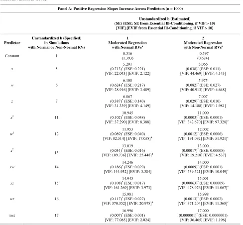
In Panel A of Table 1, the slope (b) parameters in-
crease progressively in value across the order in which predictors are specified.
[image:7.595.56.544.283.735.2]The consistent pattern of findings in Panel A must be replicated when negative slope parameters are included and when there is no pattern in the selected values of slope parameters across the order of specification. The parameters of this second type of specification could
Table 1. Monte Carlo simulations and moderated regressions of intercorrelated predictors based on normal or non-normal random variables (RVs).
Panel A: Positive Regression Slopes Increase Across Predictors (n = 1000)
Unstandardized b (Estimated)
(SE)(ESE: SE from Essential Ill-Conditioning, if VIF > 10) [VIF] [EVIF from Essential Ill-Conditioning, if VIF > 10]
Predictor
Unstandardized b (Specified) in Simulations with Normal or Non-Normal RVs
1
Moderated Regression with Normal RVsa
2
Moderated Regression with Non-Normal RVsa
Constant 1 (1.393) 0.516 (0.624) –0.597
x 5
5.291 (0.713)* (ESE: 0.221)
[VIF: 22.043] [EVIF: 2.122]
5.066 (0.038)* (ESE: 0.011)
[VIF: 44.469] [EVIF: 4.143]
w 6
6.108 (0.624)* (ESE: 0.217)
[VIF: 28.916] [EVIF: 3.489]
5.975 (0.082)* (ESE: 0.027)
[VIF: 40.913] [EVIF: 4.648]
z 7
6.867 (0.387)* (ESE: 0.140)
[VIF: 31.339] [EVIF: 4.149]
7.007 (0.029)* (ESE: 0.010)
[VIF: 14.188] [EVIF: 1.981]
x2 11 (0.102)*10.945 (ESE: 0.048)
[VIF: 37.290] [EVIF: 8.388]
11.000 (0.0003)* (ESE: 0.0001)
[VIF: 342.670] [EVIF: 97.328]c
w2 12 (0.089)*11.953 (ESE: 0.040)
[VIF: 82.514] [EVIF: 17.058]b
12.002 (0.0012)* (ESE: 0.0006)
[VIF: 191.092] [EVIF: 51.921]c
z2
13
13.019 (0.034)* (ESE: 0.016)
[VIF: 109.736] [EVIF: 25.448]b
13.000 (0.00017)* (ESE: 0.00008)
[VIF: 19.218] [EVIF: 4.537]
xw 14
14.246 (0.186)* (ESE: 0.029)
[VIF: 144.932] [EVIF: 3.584]
14.000 (0.0009)* (ESE: 0.0001)
[VIF: 539.521] [EVIF: 10.049]c
xz 15
14.945 (0.108)* (ESE: 0.017)
[VIF: 161.269] [EVIF: 3.973]
15.001 (0.00063)* (ESE: 0.00009)
[VIF: 478.976] [EVIF: 11.067]c
wz 16
15.981 (0.117)* (ESE: 0.027)
[VIF: 370.352] [EVIF: 20.978]b
15.998 (0.0013)* (ESE: 0.0002)
[VIF: 371.204] [EVIF: 11.368]c
xwz 17 (0.007)*16.996 (ESE: 0.001)
[VIF: 77.085] [EVIF: 2.024]
17.000
(0.000001)* (ESE: 0.0000001)
Continued
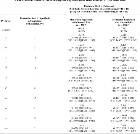
Panel B: Random Pattern of Positive and Negative Regression Slopes Across Predictors (n = 250 versus 1000)
Unstandardized b (Estimated)
(SE)(ESE: SE from Essential Ill-Conditioning, if VIF > 10) [VIF] [EVIF from Essential Ill-Conditioning, if VIF > 10]
Predictor
Unstandardized b (Specified) in Simulations with Normal RVs
1
Moderated Regression with Normal RVs
(n = 250)d
2
Moderated Regression with Normal RVs
(n = 1000)d
Constant 1 (0.492) 0.624 (0.223)0.885 *
x 2
2.350 (0.596)* (ESE: 0.148)
[VIF: 20.917] [EVIF: 1.293]
2.619 (0.251)* (ESE: 0.084)
[VIF: 14.453] [EVIF: 1.642]
w 5
5.233 (0.417)* (ESE: 0.170)
[VIF: 11.233] [EVIF: 1.605]
[image:8.595.60.533.107.559.2]5.209 (0.157)* (ESE: 0.067)
[VIF: 8.662] [EVIF: 1.597]
z –3
–2.945 (0.426)* (ESE: 0.171)
[VIF: 10.927] [EVIF: 1.765]
–3.031 (0.154)* (ESE: 0.077)
[VIF: 7.466] [EVIF: 1.897]
x2 –6 (0.062)*–6.050 (ESE: 0.030)
[VIF: 13.146] [EVIF: 3.107]
–6.006 (0.025)* (ESE: 0.012)
[VIF: 8.052] [EVIF: 2.095]
w2 4 (0.066)*4.018 (ESE: 0.029)
[VIF: 14.279 [EVIF: 2.852]
4.001 (0.018)* (ESE: 0.005)
[VIF: 9.097] [EVIF: 2.527]
z2 2 (0.060)*1.975 (ESE: 0.027)
[VIF: 9.371] [EVIF: 1.962]
2.007 (0.019)* (ESE: 0.010)
[VIF: 8.441] [EVIF: 2.554]
xw –5
–5.121 (0.284)* (ESE: 0.062)
[VIF: 41.382] [EVIF: 2.015]
–5.246 (0.123)* (ESE: 0.031)
[VIF: 37.387] [EVIF: 2.528]
xz 3
2.958 (0.190)* (ESE: 0.056)
[VIF: 36.207] [EVIF: 3.220]
2.840 (0.081)* (ESE: 0.026)
[VIF: 21.661] [EVIF: 2.265]
wz –6
–6.034 (0.148)* (ESE: 0.055)
[VIF: 20.921] [EVIF: 2.902]
–6.035 (0.047)* (ESE: 0.024)
[VIF: 22.869] [EVIF: 6.251]
xwz 2
2.031 (0.073)* (ESE: 0.011)
[VIF: 57.010] [EVIF: 1.341]
2.058 (0.029)* (ESE: 0.004)
[VIF: 42.579] [EVIF: 1.235]
*p < 0.001 (all tests are two-tailed), SE = Standard Error; ESE = Essential SE from Essential Ill-Conditioning Only; VIF = Variance Inflation Factor; EVIF =
Essential EVIF from Essential Ill-Conditioning Only.
a. In regression 1, R2 = 1, F = 99162523.48 (significant at p < 0.001). In regression 2, R2 = 1, F = 1.188 × 10¹⁵ (significant at p < 0.001).
b. In the model with normal RVs, SRC-Q results in identical b and SE estimates, while reducing all EVIF values below the cutoff score of 10. The inflated EVIF values in the SRC model for w2, z2, and wz fall to 1.589, 1.381, and 1.411, respectively, in the SRC-Q model. These deflated EVIF can be used to derive
lower ESE values for these terms.
c. In the model with non-normal RVs, SRC-Q results in identical b and SE estimates, while reducing all EVIF values below the cutoff score of 10. The inflated EVIF values in the SRC model for x2, w2, xw, xz,and wz fall to 1.010, 1.013, 1.032, 3.544, and 3.577, respectively, in the SRC-Q model. These deflated EVIF
can be used to derive lower ESE values for these terms.
d. In regression 1, R2 = 0.996, F = 6650.847 (significant at p < 0.001). In regression 2, R2 = 0.997, F = 36977.963(significant at p < 0.001). I also report the
simulation in Panel B as Table 1 in [21].
potentially be more difficult to replicate in the moderated regression, especially at smaller sample sizes, which should be detected through simulation. Therefore, I in- vestigated this possibility through the fourth simulation based on normally distributed random variables and gen- erated sample sizes of 250 and 1000. Results are reported
in Panel B of Table 1. In addition to the reported find-
In each simulation, an additional term equal to 0.4x is added to the initial distribution for w to create a final w
distribution with inessential multicollinearity (i.e., w be- comes correlated with x and with higher-order terms containing x as a component). Similarly, an additional term equal to 0.3x + 0.6w is added to the initial distribu- tion for z to create a final z distribution with inessential multicollinearity (i.e., z becomes intercorrelated with x
and w and with higher-order terms containing x and/or w
as components).
The residual term is generated as a normally distrib- uted random variable with mean = 0 and either standard deviation = 10 (Table 1, Panel A) or standard deviation
= 3 (Table 1, Panel B). For each of the two simulations
reported in each panel, the same fixed values for the b parameters from the predictor terms are used (their val- ues are listed in the first column of each panel in Table 1). I use each simulation equation to derive y based on
the generated values comprising the random variables for
x, w, z, all higher-order terms, and the residual term. All simulations were conducted using IBM SPSS Sta- tistics, version 19 (2010).
3.3. Cancer Symptoms Data and Models
These data for the secondary analyses of this study, col- lected as part of a primary study funded by the National Cancer Institute (Hospice Program Grant, CA48635), involve a sample of 268 individuals with recurrent cancer initiating outpatient palliative radiation to reduce bone pain. Medical team providers referred participants from five hospitals in a northeastern US city. Participants were at least age 30, assessed by their oncologists to be be- yond cure, although not deemed terminally ill, and had a prognosis of a year or more; they likely differed in diag- nosis/treatment stage. Men and women are almost equal- ly represented; ages range from 30 to 90, with half age 65 or older [25].
Participants provided written informed consent; the Internal Review Board approved the protocol. Structured interviews of these participants were conducted in their homes, and at four and eight months later; Schulz et al.
[25] provide additional details about the survey. I have access to a version of the initial (baseline) wave of data, which were de-identified of descriptors and variables that could lead to identification of individual participants. The Adelphi University Internal Review Board exempted these data for secondary analysis from review.
The survey included items for participant perceptions of the degree of difficulty in controlling each of several physical symptoms (each as a single item) during the
past month (the Likert-scaled categories are complete; a
lot; some; a little; none). Thus, all symptoms, including the sign of Fever, are patient-reported outcomes; object- ive measures were not also collected. The single-item measures of physical symptoms were initially reported to
be common measures derived from previous studies [25]. More recently, a review by Francoeur [26] revealed dif- ferent lines of converging evidence in the literature that collectively support the reliability and validity of self- reported, ordinal, single-item measures of the degree of control across several physical symptoms.
The survey also included all twenty items from the Center for Epidemiologic Studies-Depression (CES-D) inventory (the four ordinal categories are rarely; some of the time; much of the time; most of the time). In the cur- rent study, the dependent variable of Depressive Affect, reflecting sickness malaise during the past week, is an index of five CES-D items of negative affect (i.e., sad, blue, crying, depressed, lonely), three CES-D items of negative affect within interpersonal and situational con- texts (i.e., bothered, fearful, failure), and three reverse- coded CES-D items of positive affect (i.e., hopeful, happy, enjoyed life). CES-D somatic items were ex- cluded because they may constitute symptoms of cancer instead of depression. The internal consistency for the eleven items in these data is very good (α = 0.83), which compares favorably to α = 0.85 in the entire CES-D [26].
The data afford an opportunity to test whether pain- related interactions with fatigue and sleep problems are further co-moderated by fever in predicting depressive affect, a proxy for sickness malaise. All statistical analy- ses were conducted using IBM SPSS Statistics, version 19 (2010).
The sample of cancer symptoms provides three illus- trations of SRC, reported as QMMR models 1A, 2A, and 3A in Table 2, in which physical symptom interactions
that comprise symptom clusters predict Depressive Af- fect, a proxy for sickness malaise. In these models, the raw regression provides some of the reported statistics (i.e., b, SE, VIF) while the remaining statistics are either provided by the counterpart SRC regressions (i.e., b, EVIF) or derived from calculations based on statistics from the raw and SRC regressions (i.e., ESE). I report these and other unstandardized models in [21].
The unstandardized slope parameters from regressions 1A and 2A are used in a post hoc patient profile analysis [21] based on the Extended Zero Slopes Comparison procedure [12]. This post hoc analysis interprets the na- ture (magnifier and/or buffering) of co-moderating vari- ables on the pain-sickness malaise relationship.
Also reported within regressions 1A and 2A in Table 2 are the parameters from standardized regressions,
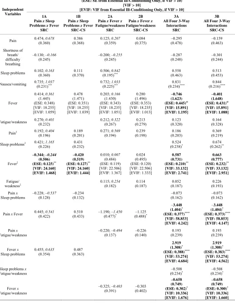
Table 2. Depressive affect predicted by physical symptoms and symptom interactionsa,b,c. Unstandardized b; Standardized b in 1A and 2A
(SE)
(ESE: SE from Essential Ill-Conditioning Only, if VIF > 10) [VIF > 10]
[EVIF: VIF from Essential Ill-Conditioning Only, if VIF > 10] Independent
Variables
1A Pain x Sleep Problems x Fever
SRC
1B Pain x Sleep Problems x Fever
SRC-CS
2A Pain x Fever x Fatigue/weakness
SRC
2B Pain x Fever x Fatigue/weakness
SRC-CS
3A All Four 3-Way
Interactions SRC
3B All Four 3-Way
Interactions SRC-CS
Pain 0.474; (0.360) 0.678 (0.368) 0.386 0.125; (0.359) 0.207 (0.375) 0.084 (0.478) –0.295 (0.463) –0.159
Shortness of breath/ difficulty breathing
–0.130; –0.166
(0.245)
–0.200; –0.255
(0.245)
–0.287 (0.248)
–0.301 (0.244)
Sleep problems 0.102; (0.360) 0.163 (0.370) 0.111 0.506; (0.195)0.842*** (0.463) 0.558 (0.453) 0.513
Nausea/vomiting 0.735; (0.231)1.037*** 0.732; (0.225)1.033*** (0.234)0.831 **** (0.216)0.844 ****
Fever
0.414; 0.361
(1.445) (ESE: 0.348) [VIF: 18.255] [EVIF: 1.059] 0.478 (1.471) (ESE: 0.351) [VIF: 18.255] [EVIF: 1.039]
0.203; 0.166
(1.430) (ESE: 0.343) [VIF: 18.235] [EVIF: 1.051] 0.280 (1.496) (ESE: 0.353) [VIF: 18.235] [EVIF: 1.013] –0.746 (1.623) (ESE: 0.445)@ [VIF: 15.891] [EVIF: 1.195]
–0.401 (1.648) (ESE: 0.431)@ [VIF: 15.891] [EVIF: 1.088]
Fatigue/weakness 0.270; (0.232) 0.401 0.212; (0.267) 0.322 (0.279) 0.213 (0.320) 0.123 (0.328) 0.164
Pain2 0.192; 0.404
(0.196)
0.189 (0.201)
0.271; 0.569
(0.194) 0.239 (0.198) 0.186 (0.203) 0.369 (0.219)
Sleep problems2 0.421; 1.165
(0.226)
0.431 (0.232)
0.524
(0.238)* (0.262)0.674 **
Fever2
–0.344; –0.244 (0.506) (ESE: 0.125)**
[VIF: 24.160] [EVIF: 1.468]
–0.420 (0.519) (ESE: 0.127)**
[VIF: 24.160] [EVIF: 1.444]
0.010; 0.007
(0.484) (ESE: 0.119) [VIF: 22.506] [EVIF: 1.367] 0.024 (0.495) (ESE: 0.120) [VIF: 22.506] [EVIF: 1.333] 0.587 (0.731) (ESE: 0.210)** [VIF: 33.132] [EVIF: 2.741]
0.663 (0.777) (ESE: 0.232)** [VIF: 33.132] [EVIF: 2.951]
Fatigue/
weakness2 0.115; (0.182) 0.254 (0.187) 0.114 (0.187) 0.052 (0.193) 0.226
Pain x
Sleep problems
–0.228; –0.537
(0.128) –0.234 (0.132) –0.073 (0.162) –0.073 (0.162)
Pain x Fever 0.445; (0.422) 0.541 (0.433) 0.510 –1.190; (0.477)–1.450* (0.488)–1.125 *
–3.448 (1.404)* (ESE: 0.377)****
[VIF: 58.853] [EVIF: 4.242]
–3.448 (1.404)* (ESE: 0.373)****
[VIF: 58.853] [EVIF: 4.147]
Pain x
Fatigue/weakness
–0.220; –0.494
(0.137) –0.226 (0.140) 0.193 (0.239) 0.193 (0.239)
Fever x
Sleep problems
0.455; 0.635
(0.354)
0.487 (0.363)
2.919 (1.308)* (ESE: 0.388)****
[VIF: 53.274] [EVIF: 4.684]
2.919 (1.308)* (ESE: 0.383)****
[VIF: 53.274] [EVIF: 4.562]
Sleep problems x
Fatigue/weakness (0.234)–0.508 * (0.234)–0.508 *
Fever x
Fatigue/weakness
–0.325; –0.403
(0.391)
–0.303 (0.402)
–0.658 (0.749) (ESE: 0.302)* [VIF: 10.336] [EVIF: 1.676]
Continued
Pain x
Sleep problems x
Fevere
–0.361; –0.732
(0.173)* (0.176)–0.377 *
–0.325 (0.327) (ESE: 0.077)****
[VIF: 20.574] [EVIF: 1.153]
–0.325 (0.327) (ESE: 0.077)****
[VIF: 20.574] [EVIF: 1.146]
Pain x
Sleep problems x
Fatigue/weakness
–0.001 (0.076)
–0.001 (0.076)
Pain x
Fever x
Fatigue/ weaknessd
0.660; 1.199
(0.243)** (0.249)0.672 **
2.105 (0.801)*** (ESE: 0.294)****
[VIF: 60.049] [EVIF: 8.067]
2.105 (0.801)*** (ESE: 0.292)****
[VIF: 60.049] [EVIF: 7.989]
Fever x
Fatigue/weakness
x Sleep problems
–1.528 (0.837)@ (ESE: 0.277)****
[VIF: 71.800] [EVIF: 7.819]
–1.528 (0.837)@ (ESE: 0.275)****
[VIF: 71.800] [EVIF: 7.730]
R2, F value 0.194, 4.663**** 0.154, 4.648**** 0.210, 5.153**** 0.160, 4.863**** 0.237, 3.711**** 0.237, 3.711****
n =268; @p < 0.10, *p < 0.05, **p < 0.01, ***p < 0.005, ****p < 0.001 (all tests are two-tailed). SE = Standard Error; ESE = Essential SE from Essential
Ill-Conditioning Only; VIF = Variance Inflation Factor; EVIF = Essential EVIF from Essential Ill-Conditioning Only. I also report 1A, 2A, and 3A in Table 3 of [21].
a. As a general rule, the VIF should not exceed 10 [27]. Cell entries in bold show dramatic reductions in inessential multicollinearity (compare VIF and EVIF) and statistically significant b parameters. Entries for a predictor are in bold when statistically non-significant b parameters in the raw regression (using SE) become significant in the SRC run (i.e., using ESE) at p < 0.05 or below, or when significant b parameters in the raw regression meet the threshold for statistical significance at a lower p value in the SRC run.
b. Separate regressions to test Fever x Fatigue/weakness x Sleep problems and Pain x Fever x Fatigue/weakness x Sleep problems (not shown) did not reveal these interactions to be statistically significant. Using SRC-Q, the coefficient of the four-way interaction switches sign (from positive to negative) and becomes significant only after excluding thirteen influential outliers; the moderate sample size may contribute to its lack of significance in the full sample. Thus, only up to three-way (second-order) regression model specifications can be taken to be valid for use with these data.
c. Influential observations with Cook’s D values greater than 4/n, or 0.140, were dropped. Two observations were dropped in 1A and 1B, one dropped in 2A and 2B, and seven dropped in 3A and 3B.
d. In 3A, in the regression specification before the last interaction is added (i.e., Fever x Fatigue/weakness x Sleep problems), the parameters for Pain x Fever x
Fatigue/weakness are statistically significant (b = 0.750, ESE = 0.111****, EVIF = 1.146). As
Table 2 reveals, the inclusion of this last interaction term in the
regression serves to dramatically increase the b parameter value for Pain x Fever x Fatigue/weakness (b = 2.105, ESE = 0.294****, EVIF = 8.067). Thus, Pain x
Fever x Fatigue/weakness is based, in part, on a “suppressor effect”. When 3A is run with all observations (i.e., including the influential cases), the suppressor effect remains as well [i.e., compare the runs: (1) with Fever x Fatigue/weakness x Sleep problems: b = 7.250, ESE = 7.562 (non-significant), EVIF = 60.049; and (2) without Fever x Fatigue/weakness x Sleep problems: b = 2.582, ESE = 1.128*, EVIF = 8.529]. The highly inflated EVIF value of 60.049 in (1) happens
to be identical to the VIF value for the same term in the raw regression that includes only non-influential observations (i.e., see regression 3A). Thus, adding the influential observations simply adds back the inessential multicollinearity removed by SRC; however, this multicollinearity now occurs within the same obser- vations (not just between the two interaction terms) and thus is now essential multicollinearity.
e. In 3A, the inclusion of Fever x Fatigue/weakness x Sleep problems creates a less dramatic suppressor effect on Pain x Sleep problems x Fever than the one on Pain x Fever x Fatigue/weakness described in footnote d. When outliers are excluded, we can compare the runs: (1) with Fever x Fatigue/weakness x Sleep problems: b = –0.325, ESE = 0.077****, EVIF = 1.153; and (2) without Fever x Fatigue/weakness x Sleep problems: b = –0.199, ESE = 0.076***, EVIF = 1.101.
When outliers are included, we can compare the runs: (3) with Fever x Fatigue/weakness x Sleep problems: b = –0.325, ESE = 0.137**, EVIF = 1.153; and (4)
without Fever x Fatigue/weakness x Sleep problems: b = –0.199, ESE = 0.167 (non-significant), EVIF = 1.101. Comparing (1) with (3) and (2) with (4), the respective b parameters and EVIF values do not change; however, the ESE values do change, such that Pain x Fever x Sleep problems ends up becoming non-significant when outliers are included. This lack of statistical significance occurs in the context of the highly inflated EVIF value of 60.049 for Pain x Fever
x Fatigue/weakness, which also became non-significant (refer to footnote d). These findings reflect overlapping variation across all three third-order interac- tions that is contributed by the set of influential observations and constitutes essential multicollinearity.
of these predictors, which is a necessary condition for direct interpretations of individual parameters based on the signed coefficient rule, the residualized variables from each sequence of the SRC are examined for low inter-correlations with the remaining predictors from the same residualizing regression.
Finally, all three QMMR models (1A, 2A, and 3A) are re-estimated to demonstrate an extension of SRC—Se- quential Residual Centering with Control and Secondary Variables (SRC-CS)—in which predictors are also con- ditioned to be uncorrelated with control and/or secondary variables. In Table 2, the resulting SRC-CS models (1B,
and both variables are dropped from 1B and 2B. How- ever, they must be retained in 3B since for any of the four three-way interactions there are additional non-re- lated lower-order polynomial terms which also serve as related terms for the other three-way interaction(s).
4. Results
4.1. Monte Carlo Simulations
This article validates a novel approach of applying re- sidual centering to regression equations that are re-esti-
mated sequentially in order to condition for multicollin-
earity across all derivative terms. This sequential resid-
ual centering (SRC) yields non-biased regression slope
parameters identical to those from uncentered regression for each order of predictor terms, as revealed in Tables 1
and 2. In simulations (n = 1000) reported in Table 1,
SRC reduces variance inflation factors (VIF) dramati-
cally, resulting in much lower values for the essential
variance inflation factors (EVIF), regardless whether all
predictors are normal or non-normal, or have similar- or
different-shaped distributions. This consistent pattern
holds, regardless whether slope parameters are positive
and increase progressively across the set of predictors,
or have no consistent pattern (based on sign and magni-
tude), even when the simulation is based on a small sam-
ple of 250. For any predictor, the EVIF is used to derive
a lower standard error of its regression slope, the essen-
tial standard error (ESE). In each simulation, the dra-
matic reductions in VIF occur along with improved con- dition matrices.
However, EVIF values for the interaction wz in the normal- and non-normal RV estimated regressions (1B and 2B in Panel A) exceed the cutoff score of 10, as does the EVIF value for the interaction xz in the non-normal RV (2B). (EVIF values of the quadratic terms are also inflated, although these might be ignored since they are not components or derivative terms of the interaction terms of interest; the quadratic terms are specified only to prevent spurious interaction effects when interaction and quadratic terms are highly correlated.) These results sug- gest that while multicollinearity is considerably reduced, some residual level may still exert some influence in both models. Even so, this remaining multicollinearity has minimal effects on findings since the regression slopes are all highly significant and very similar in value to the corresponding generated slopes of the simulation.
SRC-Q conditions away much of the remaining ines- sential multicollinearity in the normal- and non-normal estimated regressions (see Table 1, footnotes b and c).
The regression slopes and standard errors from SRC are replicated, while EVIF values across all predictors now fall below the cutoff score of 10. Recall that in SRC-Q, different terms are added to the residualizing regressions for the quadratic terms, compared to the residualizing
regressions for the one-way and interaction terms. This non-uniform residualization necessitates that the residu- alized values of the two-way quadratic terms not be specified within the same sequence of SRC-Q as the two- way interactions that contribute to the same polynomial order (i.e., second order) of terms. Thus, I specified the residualized values for the quadratic terms and the two- way interactions in separate sequences of SRC-Q.
These replicated findings mean that SRC and SRC-Q foster non-biased post hoc patient profile assessments for interpreting the nature (magnifier and/or buffering) of moderator effects at specific levels of the co-moderating variables. Indeed, biased standard errors from raw re- gression may lead a truly statistically significant slope parameter to be considered insignificant (i.e., Type II error), preventing follow-up interpretations of moderator effects where they should be made. It follows that SRC and SRC-Q also avoid Type II error in conducting non- biased direct sample-wide assessments (i.e., not requiring a separate post hoc procedure) to interpret the overall na- ture of moderator effects across the levels of co-moder- ating variables, based on the contributions of interaction terms, individually (based on the regression slope for a given interaction term) or in combination (based on the net sum of the regression slopes for multiple interaction terms and lower-order polynomial terms from which they derive), from the standardized regression.
The overall variance explained also influences the sta- tistical power for the interaction term (e.g., [11]). To test for the effect of reducing the overall variance explained, I replicate analysis 2 (n = 1000) in Table 1 panel B
across a series of increasing standard deviations of the residual term (i.e. at 10, 20, 30, 40, and 50). The R- square value deteriorated steadily from 0.996 when the standard deviation is 3 to 0.586 when the standard devia- tion is 50. As the residual term standard deviation in- creases, the extent to which the regression accurately captures the slope parameters specified in the simulation deteriorated for some of the predictors (i.e., slopes be- come biased downward for x, w, xw, and xz, although they do not change sign). However, in each case, SRC yields the same slope value as the corresponding raw regression, and when VIF exceeds 10, ESE falls appre- ciably below SE.
Next, using the small cancer sample (n = 268), I repli- cate the finding that SRC yields much lower VIF values than the raw regression, interpret direct and post hoc as- sessments in a more meaningful context with real data, and illustrate SRC-CS.
4.2. Cancer Symptom Interactions and Depressive Affect
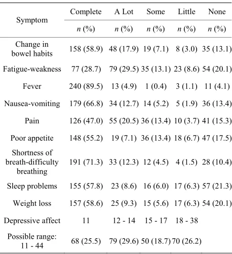
Table 3. Extent of symptom control, n = 268a.
Complete A Lot Some Little None Symptom
n (%) n (%) n (%) n (%) n (%) Change in
bowel habits 158 (58.9) 48 (17.9) 19 (7.1) 8 (3.0) 35 (13.1) Fatigue-weakness 77 (28.7) 79 (29.5) 35 (13.1) 23 (8.6) 54 (20.1)
Fever 240 (89.5) 13 (4.9) 1 (0.4) 3 (1.1) 11 (4.1)
Nausea-vomiting 179 (66.8) 34 (12.7) 14 (5.2) 5 (1.9) 36 (13.4)
Pain 126 (47.0) 55 (20.5) 36 (13.4) 10 (3.7) 41 (15.3)
Poor appetite 148 (55.2) 19 (7.1) 36 (13.4) 18 (6.7) 47 (17.5) Shortness of
breath-difficulty breathing
191 (71.3) 33 (12.3) 12 (4.5) 4 (1.5) 28 (10.4)
Sleep problems 155 (57.8) 23 (8.6) 16 (6.0) 17 (6.3) 57 (21.3)
Weight loss 157 (58.6) 25 (9.3) 15 (5.6) 17 (6.3) 54 (20.1)
Depressive affect 11 12 - 14 15 - 17 18 - 38 Possible range:
11 - 44 68 (25.5) 79 (29.6) 50 (18.7) 70 (26.2) a. Frequencies and percentages of participants experiencing symptom inter- actions when there is incomplete control (A Lot = 1 to None = 4) of each component are: Pain x Fatigue/weakness 110 (41.0); Pain x Fever 22 (8.2); Pain x Sleep Problems 141 (52.8); Fatigue/weakness x Fever 24 (9.0); Fa- tigue/weakness x Sleep Problems 190 (71.2); Fever x Sleep problems 27 (10.1); Pain x Fever x Fatigue/weakness 20 (7.5); and Pain x Fever x Sleep problems 22 (8.2). I originally reported this table as Table 2 in [26].
of all physical symptoms are highly skewed, with most participants reporting complete control of each symptom.
4.2.1. SRC with Unstandardized Predictors
Linear effects of common symptoms, quadratic effects of symptoms that are components of symptom interactions, and specific symptom interactions together predict De- pressive Affect in the regressions of Table 2. As ex-
pected, the unstandardized slope parameter estimates are
identical in the raw and SRC regressions; inflated VIF
values in the raw regression fall dramatically to EVIF values less than 10 in the SRC regressions [27]. (In Ta- ble 2, cell entries appear in bold when VIF values fall
dramatically after SRC and the unstandardized b pa- rameter becomes newly statistically significant). Fur- thermore, condition matrices from the SPSS output re- veal dramatic reductions in multicollinearity between the raw and SRC regressions. Thus, none of the predictors in the SRC runs are identified to be associated with prob- lematic multicollinearity.
In addition to meeting the common standard that all variance inflation factors (here, EVIF values) be less than 10, the EVIF in regressions 1A through 3B all meet the more conservative rule that the mean of all variance in- flation factors (here, EVIF values) from each regression must not be considerably larger than one [28]. The mean
value of 2.6 in the exhaustive three-way model tested in regression 3A suggests that while multicollinearity is dramatically reduced, remaining multicollinearity due to essential ill-conditioning could still have limited influ- ence. However, the mean value remains very similar in SRC-CS regression 3B despite additional conditioning for essential multicollinearity from secondary predictors and additional non-derivative terms based on specifica- tion of the remaining three-way interactions. In all SRC- CS regressions (1B, 2B, and 3B), the mean value remains very similar to the mean value in the corresponding SRC regression (1A, 2A, and 3A). Compared to SRC, SRC- CS yields small additional reductions in EVIF that occur only within certain lower-order predictors.
Collectively, SRC results in newly significant effects, or significance with reduced standard errors and lower p
values, based on ESE parameters, than the raw regres- sion in Table 2 (even as the relevant b and SE parame-
ters remain unchanged). Pain x Fever, Pain x Fever x
Sleep, and Pain x Fever x Fatigue/weakness—significant at p < 0.05 or 0.01 in separate three-way (second-order) explanatory models (regressions 1A, 1B, 2A, and 2B)— along with the remaining three-way term (Fever x Fa- tigue x Sleep)—all become very highly significant (p < 0.001) when all interactions are tested simultaneously (regression 3A and 3B). SRC and SRC-CS findings are similar.
The nature of the symptom interaction effects in re-
gressions 1A and 2A are probed in post-hoc patient pro- file analyses described in [21]. The interpretations, re- ported in Table 4, reveal that Fever magnifies the Pain-
Depressive Affect relationship when there is a little or no control over Sleep Problems or less than full control over Fatigue/weakness (i.e., a lot of control, a little control, no control). Furthermore, when Fever occurs, a specific range of the other co-occurring symptom (Sleep Prob- lems or Fatigue/weakness) also magnifies the Pain-De- pressive Affect relationship. Considering both magni-
fier effects together, there is a mutually synergistic and
compounded magnifier effect on the Pain-Depressive Affect relationship when Fever presents within specific ranges of either Sleep Problems (a little or no control) or Fatigue/weakness (a lot of control, a little control, no control). The relationship is buffered in the lower ranges of these two symptoms where they are better controlled.
4.2.2. SRC with Standardized Predictors
Parallel SRC models for regressions 1A and 2A are esti- mated to derive standardized slope parameters (b). These standardized slope parameters are listed in italics after the unstandardized slope parameters in Table 2. In each