http://dx.doi.org/10.4236/ojfd.2013.34041
A New Large Scale Instability in Rotating Stratified
Fluids Driven by Small Scale Forces
Anatoly Tur1, Malik Chabane1, Vladimir Yanovsky2
1Université de Toulouse [UPS], Centre National de la Recherche Scientifique,
Institut de Recherche en Astrophysique et Planétologie, Toulouse, France
2Institute for Single Crystals, National Academy of Science Ukraine, Kharkov, Ukraine
Email: [email protected]
Received October 25, 2013; revised November 25, 2013; accepted December 3, 2013
Copyright © 2013 Anatoly Tur et al. This is an open access article distributed under the Creative Commons Attribution License, which permits unrestricted use, distribution, and reproduction in any medium, provided the original work is properly cited.
ABSTRACT
In this paper, we find a new large scale instability displayed by a stratified rotating flow in forced turbulence. The tur- bulence is generated by a small scale external force at low Reynolds number. The theory is built on the rigorous as- ymptotic method of multi-scale development. There is no other special constraint concerning the force. In previous pa- pers, the force was either helical or violating parity invariance. The nonlinear equations for the instability are obtained at the third order of the perturbation theory. In this article, we explain a detailed study of the linear stage of the instabil- ity.
Keywords: Large Scale Vortex Instability; Coriolis Forse; Buoyancy; Multi-Scale Development; Small Scale Turbulence
1. Introduction
Large scale instabilities are very important in fluid dy- namics. They generate vortices which play a fundamental role in turbulence and in transport processes. The char- acteristic dimensions of the large scale structures are greater than the typical scale of the turbulence. The tur- bulence is often simulated using a small scale external force. In this case, the large scale vortices are much greater than the scale of the external force. Large scale vortices are well observed in planetary atmospheres [1, 2], in numerical simulations, and in laboratory experi- ments [3-10]. The generation process of large scale insta- bilities has been studied in several papers [11-19]. In these papers, the turbulence which generates these co- herent large scale structures cannot be homogenous, iso- tropic, or mirror invariant. A series of papers have shown that the essential mechanism which leads to the genera- tion of large scale vortices is the lack of reflection in- variance. This mechanism was called the hydrodynamic
α-effect by analogy with the similar mechanism of gen- eration of large scale magnetic fields.
Turbulence lacking reflection invariance is helical and a pseudo-scalar v r v ot 0 appears. Nevertheless, the
helicity of turbulence by itself can not generate large
scale vortices. Other factors which lack reflection inva- riance are necessary, such as, for instance, compressibil- ity [16,19] or temperature gradients [17,18]. Large scale instability can also appear if the turbulence lacks parity invariance (AKA effect) [12]. The helicity of the turbu- lence can be defined in a phenomenological way, but helicity can also be generated by an internal mechanism like rotation or buoyancy [13,15,20].
Large scale instabilities in a stratified rotating flow were studied in [21,22]. In [21], it was shown that a ro- tating incompressible flow with a constant temperature gradient can not display a large scale instability. In [22] the author presented large scale instabilities with a quad- ratic temperature gradient. In both papers, the authors used the functional averaging method. This method has some inconveniences. Especially it is impossible to make a strict hierarchy of orders as in perturbation theory. This means that it is impossible to identify the orders in which the instability appears and the ones in which it is absent. That is why the fact that the instability is absent when using the functional averaging method can not exclude its occurrence when using the rigorous asymptotic me- thod of multi-scale development.
de-velopment method in [23]. In that paper it was shown that the instability appears at the third order in the asymptotical development built on the small value of the Reynolds number. But in the first papers on this subject, using the functional averaging method, it was not clear in which order the instability would appear.
Direct numerical simulation of the Boussinesq Equa- tion confirmed the existence of large scale vortex genera- tion in stratified and rotating flows [24,25]. Sometimes the appearance of large scale vortex structures is accom- panied by an inverse cascade of energy both in the three- dimensional case (AKA-effect [26]), and in the quasi two-dimensional case [4,7,9,10]. One may say that the inverse cascade itself is also one of the mechanisms of the generation of large scale structures [5,27]. One of the important large scale instabilities in an incompressible fluid is the AKA effect (Anisotropic Kinetic Alpha effect) which was found in the work of Frisch, She and Sulem [11]. In this paper, the large scale instability appears un- der the impact of a small scale force in which parity is broken (with zero helicity). In a later paper [12], the in- verse cascade of energy and the nonlinear mode of insta- bility saturation were studied. Despite the fact that the broken parity is a more general notion than helicity, in fact, the helicity vrotv0 is the widespread mecha-
nism of symmetry breaking in hydrodynamical flows. The injection of a helical external force into a hydrody- namic system has been studied in several papers [16,19]. As a result, it was understood that a small scale turbu- lence that is able to generate large scale perturbations can not be simply homogeneous, isotropic, and helical [28], but must have additional special properties. In some cas-es, the existence of a large scale instability has been shown (a vortex dynamo or the hydrodynamic -effect). In the magneto hydrodynamics of a conductive fluid, the
-effect is well known [29]. In particular, in [17] it was shown that a large scale instability exists in convective systems with small scale helical turbulence. These papers as well as the results of numerical modelling are de- scribed in detail in the review article [30], which is fo- cused essentially on possible applications of these results to the issue of tropical cyclone origination. In this paper, we develop an analytical theory of the new large scale instability which generates large scale vortices in a strati- fied rotating flow with a constant temperature gradient under the action of a small scale external force which does not have any particular properties (especially it is nonhelical and it does not lack parity invariance). The force only maintains turbulent fluctuations. In other words, this force cannot display any instability. But the situation changes when both the Coriolis force and the buoyancy are added to this force. The joint action of these forces generates an internal helicity, which in turn generates an instability. The theory of this instability is
developed rigourously using the method of asymptotic multi-scale development similar to what was done by Frisch, She and Sulem for the theory of the AKA effect [11]. This method allows finding the equations for large scale perturbations as the secular equations of perturba- tion theory, to calculate the Reynolds stress tensor and to find the instability. Our paper is organised as follows: In Section 2, we formulate the problem and the equations for the Coriolis force and the stratification in the Boussi- nesq approximation; In Section 3, we examine the prin- cipal scheme of the multi-scale development and we give the secular equations. In Section 4, we describe the calculations of the Reynolds stress. In Section 5, we discuss the instability and the conditions for its realiza- tion. The results obtained are discussed in the conclu- sions given in Section 6. The Reynolds stress and in- ternal helicity are calculted in Appendices A and B, respectively.
2. The Main Equations and Formulation of
the Problem
Let us consider the equations for the motion of an in- compressible fluid with a constant temperature gradient in the Boussinesq approximation:
0 0
2
1 ,
t
P g T
V
V V V
V l F
(1)
z ,T
T T V A
t
V (2)
0.
V (3)
Here, l
0, 0,1
, is the thermal expansion coef-ficient, d 0 d
T A
z
is the constant equilibrium gradient of the temperature, 0Const., and T0 Al. The ex-
ternal force F0 has zero divergence. Let 0, , ,t f v0 0 0
be, respectively, the characteristic scale, time, amplitude of the external force, and velocity of our system. We choose the dimensionless variables
0 0 0
0 0
0 0 0
2 2
0 0 0 0 0
0 0 0 2 0
0 0
, , :
, , ,
, ,
, , , .
t
t t
t v
P P
f P
v v f
t P f v
x V
x V
x V
F F
2 0
0 0
0
( ) ,
1
,
Pr z
R D
t
P g T
v T
R T T RV A
t
V
V V l V
V l F
V
where R 0 0v ,D Ta
where R and
2 4 0 2 4
Ta
are respectively the Reynolds number and the Taylor number on scale 0. Pr
represents the Prandtl number. We introduce the dimensionless temperature
0 T T
A
, and obtain the system of equations
0 Pr
R D
t
Ra
P T
R
V
V V V l V
l F
1 1 .
Pr z
T T V T
R t
V
Here,
4 0Ag
Ra
is the Rayleigh number on the scale 0. Furthermore, for the purpose of simplification,
we will consider the case Pr 1 . We pass to the new temperature T T
R
, and obtain
0,
R D
t
P RaT
V
V V V l V
l F
(4)
,z T
T V R T
t
V (5)
0.
V
We will consider as a small parameter of an asymp- totic development the Reynolds number R 0 0v 1
on the scale 0. Concerning the parameters Ra and D, we do not choose any range of values for the mo- ment. Let us examine the following formulation of the problem. We consider the external force as being small and of high frequency. This force leads to small scale fluctuations in velocity and temperature against a back- ground of equilibrium. After averaging, these quickly oscillating fluctuations vanish. Nevertheless, due to small nonlinear interactions in some orders of perturbation theory, nonzero terms can occur after averaging. This means that they are not oscillatory, that is to say, they are large scale. From a formal point of view, these terms are
secular, i.e., they create the conditions for the solvability of a large scale asymptotic development. So the purpose of this paper is to find and study the solvability equations,
i.e., the equations for large scale perturbations. Let us denote the small scale variables by x0
x0,t0
, and thelarge scale ones by X
X,T
. The small scalepartial derivative operation
0 0
,
i t
x
, and the large scale
ones ,
T
X are written, respectively, as i, ,t i
and T. To construct a multi-scale asymptotic develop-
ment we follow the method which is proposed in [11].
3. The Multi-Scale Asymptotic Development
Let us search for the solution to Equations (4) and (5) in the following form:
21 0 0 1 2
3 3 1 ,
,
t X x R R
R R
V x W v v v
v
(6)
1
0
02 3
1 2 3
1 ,
,
T t T X T x
R
RT R T R T
x
(7)
3 2 1
3 2
0 0 1 1
2 3
2 3
1 1 1
,
,
P t P X P X P X
R
R R
P x R P P X
R P R P
x
(8)
Let us introduce the following equalities: 2 0
R
X x
and 4
0
T R t which lead to the expression for the space and time derivatives:
2 ,
i i
i R
x
(9) 4 ,
t R T t
(10) 2
2 4
2 .
jj j j jj
j j R R
x x
(11)
Using indicial notation, the system of the equation can be written as
4 2
2
i i j
t T j j
j k
ijk j j
R V R R V V
D l V R P
(12)
2 4
0
2 ,
,
i i i
jj j j jj
z i
t jj j
R R V RaTl F
T T V R V T
(13)
2
i 0.i R i V
(4) and (5) and then gathering together the terms of the same order, we obtain the equations of the multi- scale asymptotic development and write down the obtained equations up to order R3 inclusive. In the order R3
there is only the Equation
3 0, 3 3 .
iP P P X
(15) In order R2 we have the equation
2 0, 2 2 .
iP P P X
(16) In order R1 we get a system of equations:
1 1 1
1 3 1 1 1
1 3 1 1 1
,
,
i i j k
t jj ijk
i i j
i i j
i i j
i i j
W W D l W
P P RaT l W W
P P RaT l W W
(17)
1 1 1 1 1,
j z tT jjT jW T W
(18)
1 0. i iW
The system of Equations (17) and (18) gives the secu-lar terms
3 1i j k1,
iP RaT l Dijkl W
(19) which corresponds to a geostrophic equilibrum Equation, and
1 0. z
W (20) In zero order R0, we have the following system of
equations:
0 0 1 0 0 1 0
0 2 0 0,
i i i j i j j k
t jj j ijk
i i
i i
v v W v v W D l v
P P RaT l F
(21)
0 0 1 0 0 1 0,
j j z
tT jjT j W T v T v
(22)
0i 0. iv
These equations give one secular Equation:
2 0, 2 .
P P Const
(23)
Let us consider the equations of the first approxima-tion R:
1 1 1 1 1 1 1 0 0
1 1 1 1 1 ,
i i j k i j i j i j t jj ijk j
i j i
j i i
v v D l v W v v W v v
W W P P RaT l
(24)
1 1 1 1 1 1 0 0 1 1 1,
j j j
t jj j
j z
j
T T W T v T v T
W T v
(25)
1i i1 0. iV iW
(26) From this system of equations there follows the secu-lar equations:
1 0, i iW
(27)
1 1
1,i j
j W W iP
(28)
1 1
0.j j W T
(29) The secular equations (27) and (29) are satisfied by choosing the following geometry for the velocity field:
1 , 1 ,0 ;
1 1
;x y
W Z W Z T T Z
W (30)
1 0, 1 .
P P Const
In the second order R2, we obtain the equations
2 2 0
1 2 2 1 0 1 1 0 2
1 0 0 1 2 0 2
2
,
i i i
t jj j j
i j i j i j i j j k
j ijk
i j i j i
j i i
v v v
W v v W v v v v D l v
W v v W P P RaT l
(31)
2 2 0
1 2 2 1 0 1 1 0 1 0 0 1 2
2
,
t jj j j
j j j j
j
j j z
j
T T T
W T v T v T v T
W T v T v
(32)
2 0 0.
iv iv
(33) It is easy to see that there are no secular terms in this order..
Let us come now to the most important order R3. In
this order we obtain the equations
3 1 3 1 1
1 1 1 1 0 0
1 3 3 1 0 2 2 0 1 1 3 1
3 3
2
,
i i i i i
t T jj j j jj
i j i j i j j
i j i j i j i j i j j k
j ijk
i
i i
v W v v W
W v v W v v
W v v W v v v v v v D l v
P P RaT l
(34)
3 1 3 1 1
1 1 1 1 0 0
1 3 3 1 0 2 2 0 1 1 3 2
,
t T jj j j jj
j j j
j
j j j j j z
j
T T T T T
W T v T v T
W T v T v T v T v T v
(35)
3 1 0.
iv iv
From this we get the main secular Equation:
11 1 0 0 ,
i i k i
TW W k v v iP
(36)
1 1 0 0k 0. TT T k v T
(37) There is also an Equation to find the pressure P3:
3 1i j k1.
iP RaT l Dijkl W
(38)
4. Calculations of the Reynolds Stresses
linear alpha-effect is Equation (36). In order to obtain these equations in closed form, we need to calculate the Reynolds stresses k
v v0 0k i . First of all we have tocalculate the fields of zero approximation v0k. From the
asymptotic development in zero order we have
0 0 1 0 0
0 0 0,
i i k i j k
t jj k ijk
i i i
v v W v D l v
P RaT l F
(39)
0 0 k1 0 0k k.
tT jjT W kT v l
(40) Let us introduce the operator Dˆ0:
0
ˆ k .
t jj k
D W (41) Using Dˆ0, we rewrite Equations (39) and (40):
0 0 0 0 0 0
ˆ i j k i i,
ijk i
D v D l v P RaT l F (42)
0 0 0 ˆ k k.
D T v l (43) Eliminating the temperature and pressure from Equa- tion (42), we obtain
2
0 0 0 0 0
ˆ ˆ p k ˆ ˆ j k ˆ i.
ik ip ip pjk
D P Ral l DD P l v D F (44)
Here, Pˆip is the projection operator
ˆ i p.
ip ip jj
P
Dividing this equation by 2 0 ˆ
D , we can write it in the form
0 0
0 , ˆ
i k ik
F M v
D
(45)
where Mik is the operator given by
2
0 0
ˆ ˆ
.
ˆ ˆ
ip p k ip j
ik ik pjk
P P
M Ra l l D l
D D
(46)
We must now determine the inverse operator 1,
kj
M
. .,
i e : 1 .
ik kj ij
M M
After some calculation, we find
1
33 2
0 0
2 0
ˆ
1 ˆ
1 ˆ ˆ
ˆ
. ˆ
kp n
kj kj pjn
kp p j kj
P Ra
M P D l
D D
P
Ra l l
D
(47)
Here,
2 2
2 11 2 33 11 33 13
2 4
0 0 0
ˆ ˆ ˆ ˆ ˆ
1 ˆ ˆ
det
D Ra D Ra
P P P P P
D D D
M
(48)
and
2
11 33 13 3
0
33 13
3 3
0 0
2 2
13 11
2 2
0 0
ˆ ˆ ˆ
0 0
ˆ
ˆ 0 ˆ
ˆ ˆ
ˆ 0 ˆ
ˆ ˆ
DRa
P P P
D
DRa DRa
P P
D D
D D
P P
D D
Consequently, the expression for the velocity v0k takes
the form
33
0 2
0 0
0 2
0 0
ˆ ˆ
1
1 ˆ ˆ
ˆ
.
ˆ ˆ
kp
k n
kj pjn
j kp p j
kj P RaP
v D l
D D
P F
Ra l l
D D
(49)
In order to use these formulas, we have to specify in explicit form the external force F0j. Let us specify it by
0 f0 cos1 cos2 ,
F i k (50)
where
1 k z0 0t, 2 k x0 0t,
(51) or
1 1 0t, ,2 2 0t
k x k x (52)
1k0 0, 0,1 ; 2 k0 1, 0, 0 .
k k
One can check that F00 and F0 F0 0
Formulas (50) and (52) allow us to easily make inter- mediate calculations, but in the final formulas we obvi- ously shall take f k0, 0 and 0 as equal to unity, since
the external force is dimensionless and depends only on the dimensionless arguments of space and time. The force (50) is physically simple and can be realized in la- boratory experiments and in numerical simulations.
The force (50) can be written in complex form:
0 1 1
2 2
exp exp
exp exp ,
i i
i i
F A A
B B (53)
where A and B have the forms 0 , 0 .
2 2
f f
A i B k (54)
The effect of the operator Dˆ0 on the proper function
expi k x t has obviously the form
0 0
ˆ exp ˆ , exp
D i k x t D k i k x t ,
where Dˆ0
,k
is
20
ˆ , .
D k i k W k (55)
From this it follows that
20 1 1 1
ˆ , ,
0 1 0 1
ˆ , ˆ , ,
D D
k k (57)
20 2 2 2
ˆ , ,
D k i k W k (58)
0 2 0 2
ˆ , ˆ , .
D D
k k (59)
From Formulas (49) and (53), it follows that the field
0 k
v is composed of four terms:
0k 01k 02k 03k 04k ,
v v v v v (60) where
02 01 , 04 03 .
k k k k
v v v v
Finally, we introduce the notation
0 0 1 1 1
ˆ , 1 1 ,
D k i W D (61)
0 0 1 1
ˆ , ,
D D
k (62)
0 0 2 2 2
ˆ , 1 1 ,
D k i W D (63)
0 0 2 2
ˆ , ,
D D
k
where
W W1, 2
W Wx, y
. Taking into account theseformulas, we can write down the velocities
v
0k in the form 1 1 01 1 1 e , j i k kj A v M D
(64)
2 1 03 2 2 e , j i k kj B v M D
(65)
where 1 1 33 1 2 2
1 1 1
1
ˆ ˆ
ˆ 1 1 kj
kp n kp p j
kj pjn kj
M
P P
RaP
D l Ra l l
D D D
and 1 2 33 2 2 2
2 2 2
2 ˆ ˆ ˆ 1 1 kj
kp n kp p j
kj pjn kj
M
P P
RaP
D l Ra l l
D D D
We can now calculate the Reynolds stresses:
0 0 2 Re 01 01 03 03 ,
k i k i k
v v v vv v
(66)
which can be decomposed into two components:
0 0 1 2,
k i ki ki
v v T T (67) where T 1ki and
2 ki
T can be expressed as follows:
1 01 01 01 01,
ki k i k i
T v vv v (68)
2 03 03 03 03.
ki k i k i
T v vv v (69)
Taking into account Formulas (64) and (65), we obtain
11 33 13 2 2
1 1 1
ˆ ,ˆ ,ˆ ,ˆ .
2 2 2 i i
P P P P
We can write down the components 3 1
i
T and 3 2
i
T ,
which are the ones of interest:
2 2 2
1 1
31
1 2 6
1
, 8
D D D Ra
T
D
(70)
2 2 2
2 2
31
2 2 6
2
, 8
Ra D D D
T
D
(71)
2 3
1 32
1 2 8
1 2
, 8
D Ra D
T
D
(72)
3 3 2
2 2
32
2 2 8
2
. 8
DRa D D D
T
D
(73)
Finally, using the following relations (we have similar formulas for D2 after replacing W1 with W2):
1 1 1 1 ,
D i W (74)
2 2
1 1 1 1 ,
D W (75)
2
2
1 1 1 1 2 1 1 ,
D W i W (76)
24 2
1 1 1 1 ,
D W (77)
2
33
1 1 3 1 1 1 1 3 1 1 ,
D W i W W (78)
36 2
1 1 1 1 ,
D W (79)
48 2
1 1 1 1 ,
D W (80)
2
1 2 2
1 1
1 ,
2 2
D Ra
D D
(81)
2 1
4 2 2 2 2 2 4
1 1 1
4 1
4 2 2 2
. 4
D D Ra D D RaD Ra D
D
(82) We can then express 31
1
T , 31 2
T , 32 1
T and 32 2 T :
2 2 1 31 1 12 2 1
,
D Ra W
T
2 2 2 31 2 22 2 1
,
Ra D W
T
2 3
1 32
1
1 2 1 1
,
D Ra W
T
2 2
2 32
2
2
2 6 1
,
DRa D W
T
where
2 2
4 2 2
1,2 1 , 2
2 2
2
1,2 1,2
2[ 2 4 1 1
2 2 2 2 1 1 1 .
D Ra D Ra W
D Ra W W
5. Large Scale Instability
Let us write down in the explicit form the equations for nonlinear instability:
31 31
1 1 2 1,
TW ZT ZT W
(83)
32 32
2 1 2 2,
TW ZT ZT W
(84) where the components 31
1
T , 31 2
T , 32 1
T and 32 2
T of the Reynolds stress tensor are as defined in the previous sec- tion.
One can see that for small values of the variables W1
and W2, Equations (83) and (84) are reduced to linear
equations and describe the linear stage of instability:
1 1 2 1,
TW a ZW b ZW W
(85)
2 1 2 2,
TW c ZW d ZW W
(86) where the coeficients a, b, c and d can be written as
a b c d
a b c d
(87)
with
6 2 2 3 4 2 2
6 2
4 64 2 4
48 ,
a D D D Ra D D Ra
D D Ra
(88)
2 3 4 2
6 4 2
4 2
4 48 64 ,
b D Ra D Ra
D D D Ra
(89)
7 5 3 3 3
3 5 2 7 3
2 16 96
2 2 16 ,
c D D D D Ra
D D Ra D D Ra
(90)
3 3 5 2
7 5 3
2 2 16
2 48 32 ,
d D D Ra D D Ra
D D D D Ra
(91)
and
4 2 2
24 D Ra 2RaD 16 ,
(92) which are the explicit forms of the quite bulky coeffi-
cients. However, these coefficients can be expressed us- ing the internal helicity H0 of the velocity field v0,
calculated in Appendix B.
22 3 2
0
16 4
4
D DRa D D Ra
H
.
Therefore, we can write the constant coefficients , ,
a b c and d with respect to H0:
2 2 2 2
0 0 0 0
4 4 4 4
, , , ,
a b c d
aH b H cH d H
where 16D DRa 2
D34D Ra
2 .
Equations (85) and (86) can then be rewritten:
2 2
1 0 1 0 2 1
4 4
,
T Z Z
a b
W H W H W W
(93)
2 2
2 0 1 0 2 2
4 4
.
T Z Z
c d
W H W H W W
(94)
These formulas show that despite the zero helicity of the driving force, inside the system, an internal helicity is generated as a result of the joint impact of the Coriolis and buoyancy forces. This helicity plays an important role in the dynamics of the perturbations.
5.1. Unstable and Oscillatory Modes in the Case of Negligible Viscosity
k
1
In order to find instabilities, we choose the velocity
1, 2
W W in the form:
1 1
2 2
exp ,
exp .
W i kZ T
W i kZ T
(95)
Injecting these solutions into (85), we obtain the sim- ple system of equations:
1 2
1 2
0, 0.
ak bk
ck dk
(96)
Evidently we get a quadratic equation for :
2 a d k ad bc k2 0,
which allows us to obtain the dispersion equations for the different modes.
5.1.1. Dispersion Equation for the Unstable Mode This equation is obtained by searching for solutions of (96) for which the discriminant is negative, namely,
24 < 0
D
-10 Ra
2 4
-8 -6 -4 2 4 6 8
-4
[image:8.595.62.285.85.301.2]-2 -2
Figure 1. Instability condition with negative temperature gradient.
-1
D 30
Ra
1
0 2 3
[image:8.595.61.286.346.565.2]40 50 60 70
Figure 2. Instability condition with positive temperature gradient.
Finally, we get
0
2
2 2
0 0
, ,
4
4 4 ,
2 2
D Ra i D Ra
a d b c
a d
H k i H k
where
2 2
0
4
, 4
2
a d b c
D Ra H k
(97)
(97) is the growth rate of the instability. We note that it is proportionnal to the square of the helicity.
5.1.2. Dispersion Equation for the Oscillatory Modes This Equation is obtained by searching for solutions of (96) for which the discriminant is positive, namely,
24 > 0
a d bc .
We obtain in this case two oscillatory modes, 1 and 2
, which are, respectively, a slow and a fast mode:
22
1 0
4
4 ,
2
a d a d b c
H k
(98)
22
2 0
4
4 .
2
a d a d b c
H k
(99)
It appears that both slow and fast oscillatory frequen- cies are proportional to the square of the helicity as well.
5.2. Unstable and Oscillatory Modes with Viscosity
In the same way as before, we get the system
2
1 2
2
1 2
0, 0.
k i ak ibk
ick k i dk
(100)
We can then get a new quadratic Equation for :
2 2 4 3
2
2
0.
ik a d k k i a d k
ad bc k
Dispersion Equation for the Unstable Mode
The discriminant of this Equation is the same as in the nonviscous case, so the dispersion equation for the un- stable mode has the same condition, namely
a d
24bc< 0
, which leads to:
0 2 0
2
2 2
0
, ,
4 2
4
4 ,
2
D Ra i D Ra
a d
H k
a d b c
i H k k
where
2
2 2
0
4
, 4 .
2
a d b c
D Ra H k k
(101)
It is to be noted that the growth rate
D Ra,
ismaximal for
2
2 0
max 4
H
k ad b c
, which
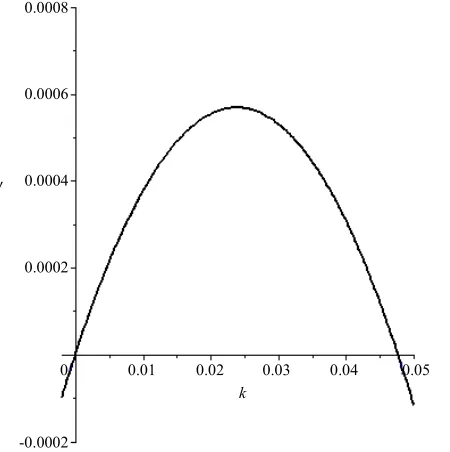
ated vortex structures. Below is Figure 3 showing the evolution of with respect to the wave number k for
1
D Ra .
It can be noted that if the discrimant is positive, we get an oscillation with an exponentially decreasing ampli- tude.
With increasing amplitude, the instability becomes nonlinear and stabilizes. As a result, nonlinear vortex struc- tures appear. The nonlinear stage of this instability and the results of numerical simulations will be presented in a future paper.
6. Conclusions and Discussion of the Results
In this paper, we showed that a large scale instability can appear in a rotating stratified fluid which is under the impact of a simple small scale external force (turbulence). The scale of this instability is much larger than the scale of the external force or turbulence. It is important to em- phasize that, unlike previous papers about large scale instabilities, in the present paper, there are no special constraints imposed on the external force. It has a zero helicity and its parity needs not be violated; this means that this is a general force. Nevertheless, the small scale turbulence under the impact of the Coriolis force and the buoyancy force becomes helical. This helicity H0, fi-
nally, is responsible for the generation of large scale in- stabilities because the growth rate is proportional to
2 0
H . The instability itself is oscillating while its fre- quency and have, in principle, the same order. This means that the instability in the general case is ape- riodic. The frequency of both the stable and unstable oscillations is also proportional to 2
0
H . So we can say
0.01 0.02 0.03 0.04 k
-0.0002 0.0002 0.0004 0.0006 0.0008
γ
[image:9.595.69.294.491.717.2]0.05 0
Figure 3. Evolution of the growth rate with respect to k .
that the oscillation modes are inertial oscillations of the rotating fluid strongly modified by the helicity. There are two oscillating modes: one slow 1 and one fast 2.
These oscillations decay when the viscosity is taken into account and in the case of instability, the maximal growth rate is reached at a characteristic scale of kmax.
Thereby this scale is typical for vortex structures like Beltrami’s runaways. In this paper, the theory of a large scale instability was constructed using the method of multi-scale developments, which was proposed in the work of Frisch, She and Sulem [11]. The nonlinear secu- lar equations for the large scale instability were obtained in the third order of development on a small Reynolds number. In this paper, we studied in detail the linear stage of the instability and the conditions of its appear- ance. It is interesting to note that instability is possible in the case of both stable and unstable stratifications. More- over, that neither the Rayleigh number nor the Taylor number are assumed to be either big or small: this means that these numbers are out of scheme parameters. That is the reason why we should state that Ra<Racr, where
cr
Ra is the critical Rayleigh number for the generation of convective instability. The unstable stratification is typical for atmosphere dynamics while the stable one is typical for ocean dynamics. We believe that the instabil- ity which was found in this paper could be applied to the issue of the generation of large scale vortices in the at- mosphere and the ocean, and to some astrophysical pro- blems as well.
REFERENCES
[1] J. Sommeria, S. P. Meyers and H. L. Swinney, “Labora- tory Simulation of Jupiter’s Great Red Spot,” Nature (London), Vol. 331, 1988, pp. 689-693.
[2] G. Dritschel and B. Legras, “Modeling Oceanic and At- mospheric Vortices,” Physics Today, Vol. 46, No. 3, 1993, p. 44.
[3] J. C. McWilliams, “The Emergence of Isolated Coherent Vortices in Turbulent Flow,” Journal of Fluid Mechanics, Vol. 146, 1984, pp. 21-43.
[4] J. Sommeria, “Experimental Study of the Two-Dimen- sional Inverse Energy Cascade in a Square Box,” Journal of Fluid Mechanics, Vol. 170, 1986, pp. 139-168.
[5] R. H. Kraichnan, “Inertial Ranges in Two-Dimensional Turbulence,” Physics of Fluids, Vol. 10, 1967, p. 1417.
[6] M. Chertkov, C. Connaughton, I. Kolokolov and V. Le- bedev, “Dynamics of Energy Condensation in Two-Di- mensional Turbulence,”Physical Review Letters, Vol. 99, 2007, Article ID: 084501.
Cascade and Turbulence Structure in Three-Dimensional Layers of Fluid,” Physics of Fluids, Vol. 23, 2011, Article ID: 095109.
[8] Y. Couder and C. Basdevant, “Experimental and Nu- merical Study of Vortex Couples in Two-Dimensional Flows,” Journal of Fluid Mechanics, Vol. 173, 1986, pp. 225-251.
[9] J. Paret and P. Tabeling, “Intermittency in the Two-Di- mensional Inverse Cascade of Energy: Experimental Ob- servations,” Physics of Fluids, Vol. 10, No. 12, 1998, p. [10] D. Molenaar, H. J. H. Clercx and G. J. F. van Heijst, “An- gular Momentum of Forced 2D Turbulence in a Square No-Slip Domain,” Physica D, Vol. 196, No. 3-4, 2007, pp. [11] U. Frisch, Z. S. She and P. L. Sulem, “Large-Scale Flow
Driven by the Anisotropic Kinetic Alpha Effect,” Physica D, Vol. 28, No. 3, 1987, pp. 382-392.
[12] P. L. Sulem, Z. S. She, H. Scholl and U. Frisch, “Genera- tion of Large-Scale Structures in Three-Dimensional Flow Lacking Parity-Invariance,” Journal of Fluid Me-chanics, Vol. 205, 1989, p. 341.
[13] G. Rudiger, “On the α-Effect for Slow and Fast Rota- tion,” Astronomische Nachrichten, Vol. 299, No. 4, 1978, pp. 217-222. [14] F. Krause and K.-H. Rädler, “Mean-Field Magnetohy-drodynamics and Dynamo Theory,” Akademie-Verlag, Berlin, 1980.
[15] H. K. Moffatt and A. Tsinober, “Helicity in Laminar and Turbulent Flow,” Annual Review of Fluid Mechanics, Vol. 24, 1992, pp. 281-312.
[16] S. S. Moiseev, R. Z. Sagdeev, A. V. Tur, G. A. Kho- menko and V. V. Yanovsky, “A Theory of Large-Scale Structure Origination in Hydrodynamic Turbulence,” So- viet Physics—JETP, Vol. 58, 1983, p. 1149.
[17] S. S. Moiseev, P. B. Rutkevich, A. V. Tur and V. V. Ya-novsky, “Vortex Dynamos in a Helical Turbulent Con- vection,” Soviet Physics—JETP, Vol. 67, 1988, p. 294. [18] E. A. Lupyan, A. A. Mazurov, P. B. Rutkevich and A. V.
Tur, “Generation of Large-Scale Vortices through the Ac-tion of Spiral Turbulence of a Convective Nature,” Soviet Physics—JETP, Vol. 75, 1992, p. 833.
[19] G. A. Khomenko, S. S. Moiseev and A. V. Tur, “The Hydrodynamic Alpha-Effect in a Compressible Fluid,” Journal of Fluid Mechanics, Vol. 225, 1991, pp. 355-369.
[20] R. Marino, P. D. Mininni, D. Rosenberg and A. Pouquet, “Emergence of Helicity in Rotating Stratified Turbu-lence,” Physical Review E, Vol. 87, 2013, Article ID: [21] Y. A. Berezin and V. P. Zhukov, “An Influence of
Rota-tion on Convective Stability of Large Scale Distorbances in Turbulent Fluid,” Izv. AN SSSR, Mech. Zhidk. Gaza, Vol. 4, 1989, p. 3.
[22] P. B. Rutkevich, “Equation for Vortex Instability Caused by Convective Turbulence and the Coriolis Force,” JETF, Vol. 77, 1993, p. 933.
[23] A. V. Tur and V. V. Yanovsky, “Non Linear Vortex Structures in Stratified Fluid Driven by Small-Scale Heli- cal Force,” Open Journal of Fluid Dynamics, Vol. 3, No. 2, 2013, pp. 64-74.
[24] L. M. Smith and F. Waleffe, “Transfer of Energy to Two- Dimensional Large Scales in Forced, Rotating Three- Dimensional Turbulence,” Physics of Fluids, Vol. 11, No. 6, 1999, p. 1608 [25] L. M. Smith and F. Waleffe, “Generation of Slow Large
Scales in Forced Rotating Stratified Turbulence,”Journal of Fluid Mechanics, Vol. 451, 2002, pp. 145-168.
[26] B. Galanti and P. L. Sulem, “Inverse Cascades in Three- Dimensional Anisotropic Flows Lacking Parity Invari- ance,” Physics of Fluids, Vol. A3, 1991, p. 1778.
[27] U. Frisch, “Turbulence: The Legacy of A. N. Kolmo- gorov,” Cambridge University Press, Cambridge, 1995. [28] F. Krause and G. Rudiger, “On the Reynolds Stress in
Mean Field Hydrodynamics. 1. Incompressible Homoge- neous Isotropic Turbulence,” Astronomische Nachrichten, Vol. 295, No. 2, 1974, pp. 93-99.
[29] H. K. Moffat, “Magnetic Field Generation in Electrically Conducting Fluids,” Cambridge University Press, Cam- bridge, 1978.
[30] G. V. Levina, S. S. Moiseev and P. B. Rutkevich, “Hy- drodynamic Alpha-Effect in a Convective System,” Ad- vances in Fluid Mechanics, Vol. 25, 2000, p. 111.
Appendix
Calculation of the Reynolds Stress Tensor
In order to calculate the Reynolds stress, we begin with the general expression
0 0 1 2
k i ki ki
v v T T (102)
with
1 01 01 01 01
ki k i k i
T v vv v (103)
and
2 03 03 03 03.
ki k i k i
T v vv v (104)
Hence,
1 1 1 1 11 1 11 1 11 1
1 1
1 1
e e e e ,
j t j t
i i i i
ki
kj it kj it
A A A A
T M M M M
D D
D D
(105)
and T 2ki has a similar expression.
Taking into account that only the components
1, 1, 3
A A B and
3
B of the external force are nonzero,
and after some factorizations, we can write the two con- tribution of the Reynolds stress tensor in the following form:
33 33
2 2
1 1
2 1
1 2 2 1 2 2 1 2 2 1
1 1 1 1
1 1 1
2 1 1 1 1 1 1
2 2 2 2
1 1 1
1 1
ˆ ˆ
1 1
ˆ
1
ˆ .
ki
i kj j i kj j i kj j
i kj j kj j it t kj j it t
RaP RaP
D D D
T A A A A P A A
D D D D
D
P A A A A A A
D D D
The same calculation for the contribution T 2ki gives us
33 33 33
3 3
2 2 2
2 2 2
3 3
2 2 2 2 2 2 2 2
2 2
2 2 2 2 2
2 2 2
33
2 2
2 3 3 3
3 3 3
2 2
2 2 2 6 2 2 2
2 2 2 2
2 2 2
ˆ ˆ ˆ
1 1 1
ˆ
ˆ 1
2 ˆ ˆ ˆ
ki
i
k k i k it t
k it t i k k it t
RaP RaP RaP
RaB RaB
D D D
T B P B P B B
D D D D D
RaP
D Ra B B RaB
B B P P P B
D D D D
3 2
3
3 2 3 2 2 2 2 2
2 2 2 2 2
2 2 2
2 2
ˆ
1
ˆ ˆ
( ) .
i kj j
k it t i kj j kj j it t kj j it t
P B
RaB
P B P B B B B B
D D D
Calculation of the Helicity
The driving force has no helicity, but the joint action of the external force, Coriolis force, and the buoyancy give the internal helicity.
The general helicity of the velocity field
v
0 is ex- pressed by
0 0 01 01 01 01
03 03 03 03 1 2,
H
H H
v v v v v v
v v v v
(106)
where we choose H 1 and H 2 such that
1 01 01 01 01
H v v v v
and
2 03 03 03 03,
H
v v v v
and in indicial notation:
0 0 v0kkui u v0i.
v v
We must calculate H with
1 1
1 1
1 1
1 1 1
1 1
1 1
1 1
1 1
e e
e e
j t
i i
kui u
kj it
j t
i i
kui u
kj it
A A
H M M
D D
A A
M M
D D
2
H is calculated in the same way, by replacing v01
with v03.
2 2
1 1 1
1
2 2
1
1
2 2
2 2
2
2 2
4 2 2
1 1
2
2 2
2
1 1
2 2
4 2 2
2 2
2
1 1 1 2 4 1 1
2 1 3 1
1 2 6 1
.
2 4 1 1
2 2 2 2 1 1 1 .
2 4 1 1
2
D W W Ra W
H
L
Ra W Ra
L
DRa W W D
L
L D Ra D Ra W
D Ra W W
L D Ra D Ra W
D
2
2 22 2
2Ra 2 2 1 W 1 1 W .
After linearization:
5 3 4 3 3
1
5 3 2 5 3
1
3 3 5 3 2
2
7 3 2 3
2
16 128 256 2
8 96 8 32 256
8 2 8 32
80 16 4
. 2
D D D DRa D Ra
H W
D D D Ra D D D Ra
W
D D Ra D D D Ra
W
D D Ra D DRa D D Ra
W
where we recall that 4
D4Ra22D Ra2 16
2.One can note that for small perturbations
W W1, 2
,the helicity approaches the constant:
2 3
0
16 4
, 2
D DRa D D Ra
H