Neural network learns from mock up operation experience:implementing on a solar energy community distribution

Neural network learns from mock-up

operation experience: implementing on

a solar energy community distribution

system with heat storage

Chih-Hsiang Lee

This dissertation is submitted for the degree of MSc by

Research of Engineering

March 2019

This thesis has not been submitted in support of an application for another degree at this or any other university. It is the result of my own work and includes nothing that is the outcome of work done in collaboration except where specifically indicated. Many of the ideas in this thesis were the product of discussion with my supervisor Dr Dénes Csala.

Chih-Hsiang Lee

Abstract

Acknowledgements

Thank you to Dr Dénes Csala of Lancaster University, UK, for advising and helpful comments on this work. Without your guidance and dedicated involvement, this paper would have never been accomplished.

I would like to express my gratitude to PVOutput online service and Energy Lancaster for providing the historical data for this research, and Gill Fenna of Quantum Strategy and Technology, UK, for helping in data collection and internship opportunity.

Contents

1 INTRODUCTION 1

1.1 Standard Model 2

1.2 Proposed Model 4

1.3 Vanilla Model 6

2 SOLAR ENERGY COMMUNITY DISTRIBUTION SYSTEM 8

2.1 Details of the System 8

2.2 Objective of Operation 10

3 OPERATION STRATEGY FOR THE COMMUNITY SYSTEM 14

4 PYTHON IMPLEMENTATION 20

4.1 Simulation Environment 20

4.2 Standard Model 21

4.3 Proposed Model 21

5 RESULTS AND DISCUSSION 26

5.1 Training result of the networks in Standard Model 26

5.2 Operation Performance 29

5.3 Annual Cost 33

5.4 Training and Computation Efficiency 40

6 CONCLUSION 42

7 REFERENCES 45

List of Tables

Table 3.1 Pseudo Code: Operation strategy for optimal operation curve 19

Table 4.1 Pseudo Code: Simulation Environment 23

Table 4.2 Pseudo Code: Standard Model 25

Table 4.3 Pseudo Code: Proposed Model 25

Table 5.1 Yearly Operation Cost 36

Table 5.2 Operation effectiveness, 𝒆𝒐𝒑 38

Table 5.3 Operation effectiveness, 𝒆_𝒐𝒑, of each week in Result 1 38

List of Figures

Figure 1.1 Concept of Standard Model 3

Figure 1.2 Training of Standard Model 4

Figure 1.3 Concept of Proposed Model 6

Figure 1.4 Training of Proposed Model 6

Figure 2.1 Solar Energy Community Distribution System 9

Figure 3.1 Expert’s Operation Curve on a cold day 18

Figure 3.2 Expert’s Operation Curve on a warm day 18

Figure 5.1 Comparisons of predictive and true values in the Standard Model 27

Figure 5.2 One-day simulation (Result 1) 31

Figure 5.3 One-day simulation (Result 2) 32

Figure 5.4 One-day simulation (Result 3) 32

List of Appendices

Appendix 1 Comparisons of predictive and true values in the Standard Model 48

Chapter 1 Introduction

1

Introduction

This paper presents a practical application of Long Short-Term Memory neural network (LSTM) [1] on a solar energy community distribution system. Unlike other models that predict features individually for supporting operators or control programmes to decide on operation actions, the proposed model in this paper was trained for directly determining the next operation action based on input features.

LSTM is capable of predicting time sequence by learning long-term dependencies in a dataset. It has the power of extracting non-linear relationship between input and output, and the capability of identifying patterns in time sequence. Thus, it has been widely used in electricity systems because key uncertainties, such PV generation, wind speed, demands and electricity price, have a temporal dependency between each time step. Many researches [2, 3, 4, 5, 6, 7] applied LSTM purely to predict key features related to electricity industry, such as weather condition, electricity prices, and energy demands. These predictions can be used to support operator’s decision making, but not directly

provide operation actions on the electricity equipment or systems.

LSTM was implemented only to predict the uncertainty, such as future inflow of each wastewater treatment plant or sewer. Similarly, LSTM predictions made in [8, 9] have no connection to their proposed strategies, but only provide better information to operators who use those strategies.

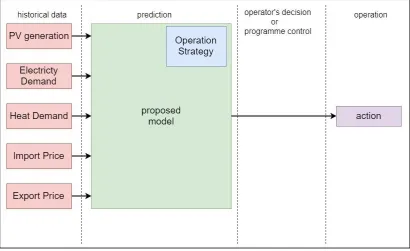
In this paper, we built three models to compare the performance of conventional and our proposed method. Standard Model adopted the idea discussed above that forecast only serves as a reference in operating the system. Operators or control programmes accept the forecast and run the operation strategy to determine the current action. On the contrary, our Proposed Model integrates the operation strategy into its training set, enabling the model to directly control the system. Simulative results show that the Proposed Model outperforms the Standard Model. Moreover, even though the Proposed Model takes more resources to prepare the training set, no calculation need to be done when processing online. In the long run, the Proposed Model consumes less processing time than the Standard Model. Last, for comparison, the Vanilla Model follows a common strategy that the storage always starts at fixed times to be charged or to be discharged.

Note that when we use the word, ‘operator,’ in this paper, it usually means the same as ‘control programme’ since the three Models are controlled by computer programmes.

1.1

Standard Model

Applying the concept mentioned above, we build a Standard Model to provide a basis for comparison to the Proposed Model. This concept is a straightforward implementation of LSTM networks on operation of systems with uncertainty and has been adopted by many researches.

Chapter 1 Introduction

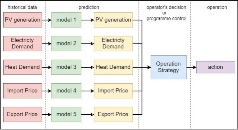
in Figure 2.1 and detailed in Chapter 2. Each sub-model (green square) in Figure 1.1 has one LSTM network. In the beginning of every half hour, each sub-model accepts input from historical data to make prediction of five key features relevant to operation decision: PV generation, electricity demand, heat demand, importing price of the grid and exporting price of the grid. A computer programme that follows operating strategy (blue square) then accepts those predictions as input for calculating the operation action in current half hour.

Figure 1.1 Concept of Standard Model

Figure 1.2 Training of Standard Model

1.2

Proposed Model

To design our Proposed Model, we first formulated an operating strategy that determines the target level of heat storage every half hour, based on the five input features. Following our proposed strategy, the heat storage will be charged if its current energy level is less than the target level. Charging can be done not only by PV generation but also electricity imported from the grid if future importing price is expected to become higher. If the current energy level is more than the target level, the heat storage discharges. This proposed strategy is designed to decrease total operation cost, detailed in Section 2.2. To make the comparison meaningful, ‘Operation Strategy (blue square)’ in Figure 1.1 is the same as our proposed operating strategy of heat storage in Figure 1.3.

To utilise the proposed strategy, uncertainties of the five input features must be eliminated. Instead of training five LSTM sub-models that predict these features, we trained only one LSTM model that takes these five features as inputs to directly output a target level for every half hour.

We applied the principle behind Imitation Learning, of which a model learns from expert’s behaviours. For example, when learning self-driving cars, a model is showed

Chapter 1 Introduction

Those demonstrated actions are recorded from an expert, such as a human driver. Imitation Learning is usually implemented when calculation of an action is impossible or too expensive, but the task is easy for a human to perform. In our case, although no person can perfectly predict future when operating heat storage, we can create a mock-up expert from historical data. This expert follows the proposed strategy in simulations of operating a system. The expert’s behaviours are then used as the training set for the Proposed Model.

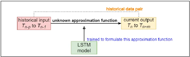
The training method of the Proposed Model is showed in Figure 1.4. In contrast to the training pairs for the Standard Model in Figure 1.2, the Proposed Model learns to interpret the relationship between a time sequence and one output value. The training pairs in Figure 1.4 are ‘handcrafted’ by following the proposed strategy. Consequently, the Proposed Model is connected to the proposed strategy itself, and its output is directly determining the next operation action.

Figure 1.3 Concept of Proposed Model

Figure 1.4 Training of Proposed Model

1.3

Vanilla Model

Chapter 1 Introduction

Therefore, we set the Vanilla Model always charge and discharge at these two times every day. The storage is charged and discharged with a fix rate.

Another key difference between the Vanilla Model and other two models is that during charging the Vanilla Model never imports electricity from the grid if PV-generation is not enough because the Vanilla Model have no ability to forecast electricity price. It would end up in excessive expenditure if allowing the Vanilla Model to import electricity. When there’s no PV-generation during charging, the Vanilla Model would stop charging the

storage until PV-generation resumes.

2

Solar Energy Community

Distribution System

2.1

Details of the System

Chapter 2 Solar Energy Community Distribution System

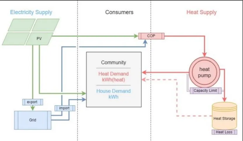
Figure 2.1 Solar Energy Community Distribution System

If PV generation is insufficient to cover heat demand, the short of heat supply is compensated by importing electricity from the grid to run heat pumps or by discharging heat from the storage. When heat pumps run out of capacity, the only way to provide heat is discharging the storage. In this paper, we assume that heat pump capacity is always sufficient to cover demand peak. The heat pump capacity is set to be a little high than the maximum heat demand in our simulative environment, but not infinite.

Finally, excess PV generation can be sold to the grid, or be used to charge heat storage if heat pumps still has capacity. In this study, we assume that domestic use of PV generation is always more economical than selling to the grid.

In each half hour there are two prices: System Sell Price (SSP) and System Buy Price (SBP). When the operator imports electricity from the grid, the operator needs to pay the SBP. Likewise, the grid pays the SSP to the operators who export electricity to the grid. These two prices are called ‘imbalance prices’ and originally designed to tackle the deficit

of imbalance energy. In our study, we use a historical data of SSP and SBP around Lancaster area to simulate the price change faced by operators.

2.2

Objective of Operation

In our system, PV generation is always used to meets electricity demand first and then heat demand. After that if any PV generation remains, it can be used to charge the storage or be sold to the grid. Thus, we defined ‘PV Surplus’ as the amount of remaining PV

generation we can manipulate:

𝑷𝑽 𝑺𝒖𝒓𝒑𝒍𝒖𝒔 = 𝑷𝑽 𝒈𝒆𝒏𝒆𝒓𝒂𝒕𝒊𝒐𝒏 − 𝒆𝒍𝒆𝒄𝒕𝒓𝒊𝒄𝒊𝒕𝒚 𝒅𝒆𝒎𝒂𝒏𝒅 − (𝒉𝒆𝒂𝒕 𝒅𝒆𝒎𝒂𝒏𝒅 ÷ 𝑪𝑶𝑷) ( 1 )

𝒊𝒇 𝑷𝑽 𝑺𝒖𝒓𝒑𝒍𝒖𝒔 < 𝟎, 𝑷𝑽 𝑺𝒖𝒓𝒑𝒍𝒖𝒔 = 𝟎

When PV generation is unable to cover all heat demand, we defined a term ‘Shortage’ as the amount of remaining heat demand that we need to cope with by heat storage:

𝑺𝒉𝒐𝒓𝒕𝒂𝒈𝒆 = 𝒉𝒆𝒂𝒕 𝒅𝒆𝒎𝒂𝒏𝒅 − [(𝑷𝑽 𝒈𝒆𝒏𝒆𝒓𝒂𝒕𝒊𝒐𝒏 − 𝒆𝒍𝒆𝒄𝒕𝒓𝒊𝒄𝒊𝒕𝒚 𝒅𝒆𝒎𝒂𝒏𝒅) × 𝑪𝑶𝑷] ( 2 )

𝒊𝒇(𝑷𝑽 𝒈𝒆𝒏𝒆𝒓𝒂𝒕𝒊𝒐𝒏 − 𝒆𝒍𝒆𝒄𝒕𝒓𝒊𝒄𝒊𝒕𝒚 𝒅𝒆𝒎𝒂𝒏𝒅) < 𝟎, 𝑺𝒉𝒐𝒓𝒕𝒂𝒈𝒆 = 𝒉𝒆𝒂𝒕 𝒅𝒆𝒎𝒂𝒏𝒅

𝒊𝒇 𝑺𝒉𝒐𝒓𝒕𝒂𝒈𝒆 < 𝟎, 𝑺𝒉𝒐𝒓𝒕𝒂𝒈𝒆 = 𝟎

Chapter 2 Solar Energy Community Distribution System

capability to forecast future electricity prices to know when the best time to buy electricity is. Furthermore, the operator must be able to forecast future PV generation and demands to determine what is the actual amount of heat needed to be prepared in advanced. For example, if a sunny day is expected, the operator has no need to import electricity to charge the storage even though current SBP is low

The goal of the operator is to reduce operation cost of the system. Operation cost is equal to the expenditure of importing electricity from the grid subtracted by the income of selling PV generation to the grid. In terms of cost, income is negative:

𝑶𝒑𝒆𝒓𝒂𝒕𝒐𝒊𝒏 𝒄𝒐𝒔𝒕 = 𝒆𝒙𝒑𝒆𝒏𝒅𝒊𝒕𝒖𝒓𝒆 𝒐𝒇 𝒊𝒎𝒑𝒐𝒓𝒕𝒊𝒏𝒈 + (−𝒊𝒏𝒄𝒐𝒎𝒆 𝒐𝒇 𝒆𝒙𝒑𝒐𝒓𝒕𝒊𝒏𝒈) ( 3 )

With heat storage and a good predictor of future PV generation, demands and system prices, the operator can accomplish several tasks to decrease operation cost:

A. If the operator has PV surplus in the current moment and expects a Shortage in a future moment and importing electricity with future SBP is expensive than not selling PV surplus with current SSP, the operator should charge the storage with current PV surplus:

(𝒊) 𝑺𝒆𝒍𝒍𝒊𝒏𝒈 𝑷𝑽 𝒔𝒖𝒓𝒑𝒍𝒖𝒔 𝒓𝒊𝒈𝒉𝒕 𝒏𝒐𝒘, 𝒂𝒏𝒅 𝒊𝒎𝒑𝒐𝒓𝒕𝒊𝒏𝒈 𝒆𝒍𝒆𝒄𝒕𝒓𝒊𝒄𝒊𝒕𝒚 𝒊𝒏 𝒕𝒉𝒆 𝒇𝒖𝒕𝒖𝒓𝒆:

𝒊𝒏𝒄𝒐𝒎𝒆 = −𝑷𝑽 𝒔𝒖𝒓𝒑𝒍𝒖𝒔 × 𝒄𝒖𝒓𝒓𝒆𝒏𝒕 𝑺𝑺𝑷

𝒆𝒙𝒑𝒆𝒏𝒅𝒊𝒕𝒖𝒓𝒆 = [𝑺𝒉𝒐𝒓𝒕𝒂𝒈𝒆 ÷ 𝑪𝑶𝑷] × 𝒇𝒖𝒕𝒖𝒓𝒆 𝑺𝑩𝑷

(𝒊𝒊) 𝑺𝒂𝒗𝒊𝒏𝒈 𝑷𝑽 𝒔𝒖𝒓𝒑𝒍𝒖𝒔 𝒓𝒊𝒈𝒉𝒕 𝒏𝒐𝒘 𝒇𝒐𝒓 𝒕𝒉𝒆 𝒇𝒖𝒕𝒖𝒓𝒆:

𝒊𝒏𝒄𝒐𝒎𝒆 = 𝟎 𝒆𝒙𝒑𝒆𝒏𝒅𝒊𝒕𝒖𝒓𝒆 = 𝟎

𝒊𝒇 𝑶𝒑𝒆𝒓𝒂𝒕𝒊𝒐𝒏 𝒄𝒐𝒔𝒕(𝒊𝒊) − 𝑶𝒑𝒆𝒓𝒂𝒕𝒊𝒐𝒏 𝒄𝒐𝒔𝒕(𝒊) < 𝟎:

→ 𝟎 − (−𝑷𝑽 𝒔𝒖𝒓𝒑𝒍𝒖𝒔 × 𝒄𝒖𝒓𝒓𝒆𝒏𝒕 𝑺𝑺𝑷 + [𝑺𝒉𝒐𝒓𝒕𝒂𝒈𝒆 ÷ 𝑪𝑶𝑷] × 𝒇𝒖𝒕𝒖𝒓𝒆 𝑺𝑩𝑷) < 𝟎 → 𝑷𝑽 𝒔𝒖𝒓𝒑𝒍𝒖𝒔 × 𝒄𝒖𝒓𝒓𝒆𝒏𝒕 𝑺𝑺𝑷 < [𝑺𝒉𝒐𝒓𝒕𝒂𝒈𝒆 ÷ 𝑪𝑶𝑷] × 𝒇𝒖𝒕𝒖𝒓𝒆 𝑺𝑩𝑷

→ 𝑷𝑽 𝒔𝒖𝒓𝒑𝒍𝒖𝒔 × 𝒄𝒖𝒓𝒓𝒆𝒏𝒕 𝑺𝑺𝑷 < 𝑷𝑽 𝒔𝒖𝒓𝒑𝒍𝒖𝒔 × 𝒍𝒐𝒔𝒔(𝒕𝒇𝒖𝒕𝒖𝒓𝒆−𝒕𝒄𝒖𝒓𝒓𝒆𝒏𝒕)_{× 𝒇𝒖𝒕𝒖𝒓𝒆 𝑺𝑩𝑷}

→ 𝒄𝒖𝒓𝒓𝒆𝒏𝒕 𝑺𝑺𝑷 ÷ 𝒍𝒐𝒔𝒔(𝒕𝒇𝒖𝒕𝒖𝒓𝒆−𝒕𝒄𝒖𝒓𝒓𝒆𝒏𝒕)_{< 𝒇𝒖𝒕𝒖𝒓𝒆 𝑺𝑩𝑷 ( 4 )}

, where 𝑡_{𝑓𝑢𝑡𝑢𝑟𝑒}− 𝑡_{𝑐𝑢𝑟𝑟𝑒𝑛𝑡} is the difference between current and future time. And

𝑙𝑜𝑠𝑠 is the heat loss in storage per unit time. In our study, the unit time is equal to

a half hour, and transition loss is ignored for simplification.

B. If the operator has no PV surplus in the current moment and expects a Shortage in a future moment and importing electricity with future SBP is expensive than importing electricity with current SBP, the operator should import electricity with current SBP to charge the storage.

(𝒊) 𝑫𝒐 𝒏𝒐𝒕𝒉𝒊𝒏𝒈 𝒓𝒊𝒈𝒉𝒕 𝒏𝒐𝒘, 𝒂𝒏𝒅 𝒊𝒎𝒑𝒐𝒓𝒕𝒊𝒏𝒈 𝒆𝒍𝒆𝒄𝒕𝒓𝒊𝒄𝒊𝒕𝒚 𝒊𝒏 𝒕𝒉𝒆 𝒇𝒖𝒕𝒖𝒓𝒆:

𝒆𝒙𝒑𝒆𝒏𝒅𝒊𝒕𝒖𝒓𝒆𝒄𝒖𝒓𝒓𝒆𝒏𝒕= 𝟎

𝒆𝒙𝒑𝒆𝒏𝒅𝒊𝒕𝒖𝒓𝒆𝒇𝒖𝒕𝒖𝒓𝒆= [𝑺𝒉𝒐𝒓𝒕𝒂𝒈𝒆 ÷ 𝑪𝑶𝑷] × 𝒇𝒖𝒕𝒖𝒓𝒆 𝑺𝑩𝑷

(𝒊𝒊) 𝑰𝒎𝒑𝒐𝒓𝒕𝒊𝒏𝒈 𝒆𝒍𝒆𝒄𝒕𝒓𝒊𝒄𝒊𝒕𝒚 𝒓𝒊𝒈𝒉𝒕 𝒏𝒐𝒘 𝒇𝒐𝒓 𝒕𝒉𝒆 𝒇𝒖𝒕𝒖𝒓𝒆:

𝒆𝒙𝒑𝒆𝒏𝒅𝒊𝒕𝒖𝒓𝒆𝒄𝒖𝒓𝒓𝒆𝒏𝒕= 𝑰𝒎𝒑𝒐𝒓𝒕𝒊𝒏𝒈 𝒆𝒍𝒆𝒄𝒕𝒓𝒊𝒄𝒊𝒕𝒚 × 𝒄𝒖𝒓𝒓𝒆𝒏𝒕 𝑺𝑩𝑷

𝒆𝒙𝒑𝒆𝒏𝒅𝒊𝒕𝒖𝒓𝒆𝒇𝒖𝒕𝒖𝒓𝒆= 𝟎

(𝑨𝒔𝒔𝒖𝒎𝒊𝒏𝒈: 𝑰𝒎𝒑𝒐𝒓𝒕𝒊𝒏𝒈 𝒆𝒍𝒆𝒄𝒕𝒓𝒊𝒄𝒊𝒕𝒚 × 𝑪𝑶𝑷 × 𝒍𝒐𝒔𝒔(𝒕𝒇𝒖𝒕𝒖𝒓𝒆−𝒕𝒄𝒖𝒓𝒓𝒆𝒏𝒕) _{= 𝑺𝒉𝒐𝒓𝒕𝒂𝒈𝒆)}

𝒊𝒇 𝑶𝒑𝒆𝒓𝒂𝒕𝒊𝒐𝒏 𝒄𝒐𝒔𝒕(𝒊𝒊) − 𝑶𝒑𝒆𝒓𝒂𝒕𝒊𝒐𝒏 𝒄𝒐𝒔𝒕(𝒊) < 𝟎:

→ 𝑰𝒎𝒑𝒐𝒓𝒕𝒊𝒏𝒈 𝒆𝒍𝒆𝒄𝒕𝒓𝒊𝒄𝒊𝒕𝒚 × 𝒄𝒖𝒓𝒓𝒆𝒏𝒕 𝑺𝑩𝑷 − [𝑺𝒉𝒐𝒓𝒕𝒂𝒈𝒆 ÷ 𝑪𝑶𝑷] × 𝒇𝒖𝒕𝒖𝒓𝒆 𝑺𝑩𝑷 < 𝟎

→ 𝑰𝒎𝒑𝒐𝒓𝒕𝒊𝒏𝒈 𝒆𝒍𝒆𝒄𝒕𝒓𝒊𝒄𝒊𝒕𝒚 × 𝒄𝒖𝒓𝒓𝒆𝒏𝒕 𝑺𝑩𝑷 < [𝑺𝒉𝒐𝒓𝒕𝒂𝒈𝒆 ÷ 𝑪𝑶𝑷] × 𝒇𝒖𝒕𝒖𝒓𝒆 𝑺𝑩𝑷

→ 𝑰𝒎𝒑𝒐𝒓𝒕𝒊𝒏𝒈 𝒆𝒍𝒆𝒄𝒕𝒓𝒊𝒄𝒊𝒕𝒚 × 𝒄𝒖𝒓𝒓𝒆𝒏𝒕 𝑺𝑩𝑷

< 𝑰𝒎𝒑𝒐𝒓𝒕𝒊𝒏𝒈 𝒆𝒍𝒆𝒄𝒕𝒓𝒊𝒄𝒊𝒕𝒚 × 𝒍𝒐𝒔𝒔(𝒕𝒇𝒖𝒕𝒖𝒓𝒆−𝒕𝒄𝒖𝒓𝒓𝒆𝒏𝒕)_{× 𝒇𝒖𝒕𝒖𝒓𝒆 𝑺𝑩𝑷}

Chapter 2 Solar Energy Community Distribution System

C. If the operator expects several available electricity sources at 𝑡₁, 𝑡₂, 𝑡₃, 𝑡₄, and a Shortage at 𝑡5, the operator must compare the prices, which are modified by loss and different time spans. The modified prices could be:

{𝒄𝒖𝒓𝒓𝒆𝒏𝒕 𝑺𝑺𝑷 ÷ 𝒍𝒐𝒔𝒔

(𝒕𝒇𝒖𝒕𝒖𝒓𝒆−𝒕𝒄𝒖𝒓𝒓𝒆𝒏𝒕)_{, 𝒊𝒇 𝒕𝒉𝒆 𝒔𝒐𝒖𝒓𝒄𝒆 𝒊𝒔 𝑷𝑽 𝒔𝒖𝒓𝒑𝒍𝒖𝒔}

𝒄𝒖𝒓𝒓𝒆𝒏𝒕 𝑺𝑩𝑷 ÷ 𝒍𝒐𝒔𝒔(𝒕𝒇𝒖𝒕𝒖𝒓𝒆−𝒕𝒄𝒖𝒓𝒓𝒆𝒏𝒕)_{, 𝒊𝒇 𝒕𝒉𝒆 𝒔𝒐𝒖𝒓𝒄𝒆 𝒊𝒔 𝒊𝒎𝒑𝒐𝒓𝒕𝒊𝒏𝒈 𝒆𝒍𝒆𝒄𝒕𝒓𝒊𝒄𝒊𝒕𝒚}

3

Operation Strategy for the

Community System

With historical data, we can assume that there is a perfect predictor, “an expert,” who can

forecast all we need in next 24 hours, which is divided equally into 𝑡₀ to 𝑡₄₇. Our operation strategy is to analyse the relationship of PV surplus, Shortage, SSP and SBP at 𝑡0 to 𝑡47, to determine the profitability of each available electricity source and to distribute all available electricity sources to all Shortage at 𝑡₀ to 𝑡₄₇ accordingly. Available electricity sources include PV Surplus and importing electricity from the grid.

At the start of 𝑡0, the expert holds the values of PV surplus, Shortage, SSP and SBP at 𝑡0 to 𝑡47. First, it creates a profit table, in which each entry is called a ‘profit number’:

𝒑𝒓𝒐𝒇𝒊𝒕 𝒏𝒖𝒎𝒃𝒆𝒓

= {(𝑺𝑺𝑷𝒑÷ 𝒍𝒐𝒔𝒔

(𝒕𝒏−𝒕𝒑)_{) ÷ 𝑺𝑩𝑷}

𝒏 , 𝒊𝒇 𝒖𝒔𝒊𝒏𝒈 𝑷𝑽 𝑺𝒖𝒓𝒑𝒍𝒖𝒔 𝒂𝒕 𝒕𝒑 𝒕𝒐 𝒄𝒉𝒂𝒓𝒈𝒆 𝒉𝒆𝒂𝒕 𝒔𝒕𝒐𝒓𝒂𝒈𝒆

(𝑺𝑩𝑷𝒑÷ 𝒍𝒐𝒔𝒔(𝒕𝒏−𝒕𝒑)) ÷ 𝑺𝑩𝑷𝒏 , 𝒊𝒇 𝒊𝒎𝒑𝒐𝒓𝒕𝒊𝒏𝒈 𝒆𝒍𝒆𝒄𝒕𝒓𝒊𝒄𝒊𝒕𝒚 𝒂𝒕 𝒕𝒑 𝒕𝒐 𝒄𝒉𝒂𝒓𝒈𝒆 𝒉𝒆𝒂𝒕 𝒔𝒕𝒐𝒓𝒂𝒈𝒆

, where 𝑡_𝑛 > 𝑡_𝑝 and 𝑡_𝑛, 𝑡_𝑝 ∈ 𝑡₀ to 𝑡₄₇. 𝑆𝑆𝑃_𝑝 is the SSP at 𝑡_𝑝, 𝑆𝐵𝑃_𝑝 is the SBP at 𝑡_𝑝 and

𝑆𝐵𝑃𝑛 is the SBP at 𝑡𝑛. We only consider 𝑡𝑛 when there is a Shortage at 𝑡𝑛.

We set 𝑝𝑓_𝑝,𝑛𝑃𝑉 be the profit number when using PV Surplus at 𝑡_𝑝 to charge heat storage for

future Shortage at 𝑡_𝑛 . Similarly, 𝑝𝑓_𝑝,𝑛𝐺𝑑 _{is the profit number when importing electricity} from the grid at 𝑡_𝑝 to charge heat storage for future Shortage at 𝑡_𝑛 . Refer to Equation (4)

and (5), it is obvious that if 𝑝𝑓𝑝,𝑛 < 1, it’s profitable to use electricity source at 𝑡𝑝 . On

the other hand, if 𝑝𝑓_𝑝,𝑛 ≥ 1, it has no need to use electricity source at 𝑡_𝑝 and this 𝑝𝑓_𝑝,𝑛

would be excluded from the profit table.

Chapter 3 Operation Strategy for the Community System

Next, the expert distributes all available electricity source to all Shortage, starting from the smallest 𝑝𝑓_𝑝,𝑛. The expert calculates the exact amount of electricity needed at 𝑡_𝑝 for the Shortage at 𝑡_𝑛 :

𝒆𝒍𝒆𝒄𝒕𝒓𝒊𝒄𝒊𝒕𝒚 𝒓𝒆𝒒𝒖𝒊𝒓𝒎𝒆𝒏𝒕 𝒂𝒕 𝒕𝒑= (𝑺𝒉𝒐𝒓𝒕𝒂𝒈𝒆 𝒂𝒕 𝒕𝒏÷ 𝒍𝒐𝒔𝒔(𝒕𝒏−𝒕𝒑)) × 𝑪𝑶𝑷 ( 7 )

The expert then adjusts the electricity requirement at 𝑡_𝑝 according to heat pump capacity at 𝑡_𝑝 and heat storage capacity at 𝑡_𝑝, 𝑡_𝑝+1, 𝑡_𝑝+2,……, and 𝑡_𝑛 because heat pump capacity

limits the amount of heat that can be charged, and heat storage capacity limits the amount of heat that can be stored in the heat storage.

Finally, the expert decreases the electricity source at 𝑡_𝑝 as much as possible according to

the modified electricity requirement at 𝑡𝑝. If the electricity source is PV Surplus, the

expert records how much amount of PV Surplus remains. If the electricity source is from the grid, the expert can import as much as it need, because we assume that the connection to the grid is always available. The amount of electricity consumed at 𝑡𝑝 turns into heat, which reduces heat pump capacity at 𝑡_𝑝. The expert also records the decrease of Shortage at 𝑡_𝑛 and the decreases of heat storage capacity at 𝑡_𝑝, 𝑡_𝑝+1, 𝑡_𝑝+2,……, and 𝑡_𝑛.

To increase the efficiency of the algorithm, when a heat pump capacity at 𝑡𝑝 is exhausted,

all 𝑝𝑓_𝑝,𝑛 with 𝑡_𝑝 will be deleted from the profit table. Similarly, when a heat storage capacity at 𝑡_𝑥 is used up, all 𝑝𝑓_𝑝,𝑛 with 𝑡_𝑝 ≤ 𝑡_𝑥≤ 𝑡_𝑛 will be deleted. In addition, after a

Shortage at 𝑡𝑛 is fully fulfilled, all 𝑝𝑓𝑝,𝑛 with 𝑡𝑛 will be deleted.

In Figure 3.1 and Figure 3.2, the heat level of heat storage (purple dot) of 𝑡_𝑛 is the heat level at the start of 𝑡𝑛, and the bars (orange and indigo) show how much amount of heat is charged into the storage at the end of 𝑡_𝑛. For example, at the start of 𝑡₀ and 𝑡₁ in Figure 3.1 there is no heat in the storage, and the operator charges the storage by 243.18 kWh during 𝑡1. Thus, at the start of 𝑡2 the heat level is equal to 243.18 kWh as showed in the figure.

Note that PV generation in Figure 3.1 and Figure 3.2 has been subtracted by electricity demand first and then converted to heat energy for clearly demonstrating how PV generation is used to charge the storage.

The operation curves in Figure 3.1 and Figure 3.2 demonstrate several behaviours that our Proposed Model must learn:

A. Avoid storing excessive heat:

Comparing the sum of heat demand from 𝑡12 and 𝑡17(approx. 771.36 kWh) and the total heat released from the heat storage from 𝑡12 and 𝑡17 (approx. 762.98 kWh) in Figure 3.1, it can be seen that heat prepared in the storage is slightly less than the heat demand because it can be covered by the PV generation at 𝑡₁₇ (approx. 8.38 kWh). After that, heat demand from 𝑡18 and 𝑡29 is fully covered by PV generation. This behaviour demonstrates that our expert knows the optimal amount of heat that needs to be prepared before a certain time, depending on when PV generation begins and what amount of PV generation occurs in the future.

Likewise, expecting a low demand during the evening in Figure 3.2, the expert fills the storage to a sufficient amount of heat (approx. 794.52 kWh), but not to its full capacity (1500 kWh). This shows the expert’s capability of operating the storage

Chapter 3 Operation Strategy for the Community System

B. Charge the storage economically:

Figure 3.1 Expert’s Operation Curve on a cold day

Chapter 3 Operation Strategy for the Community System

4

Python Implementation

We use Python and Jupyter Notebook to create the Models and to conduct simulations. The implement of LSTM networks is constructed by Keras, a neural networks API of Python [10].

4.1

Simulation Environment

The pseudo code of simulation environment is showed in Table 4.1.

We first set up a four-year database of the five features (PV generation, electricity and heat demand, SSP and SBP):

A. PV generation is based on a four-year real data.

B. We assumed that electricity demand per dwelling per year is set to be 3000 kWh and there are 180 houses in the community. Electricity demand curve is based on a one-year real data.

C. Heat demand per dwelling is set to be 4500 kWh. Heat demand curve is based on a one-year estimated data.

D. SBP and SSP are based on a one-year real data. The average of SBP is 0.04756 £/kW, and of SSP is 0.0366 £/kWh. SBP is always greater than or equal to SSP.

Chapter 4 Python Implementation

4.2

Standard Model

In Standard Model, we trained five networks to predict each feature (PV generation, heat demand, electricity demand, SSP and SBP). Each network receives a value sequence of 𝑡_𝑛−48 to 𝑡_𝑛−1 to forecast the sequence of 𝑡_𝑛 to 𝑡_𝑛+47, as showed in Figure 1.2, in which 𝑝 = 48 and 𝑚 = 47. The operator then put these predicted sequences of 𝑡_𝑛 to 𝑡_𝑛+47 into Algorithm 1 (Table 3.1) to determine the target level of heat storage at 𝑡_𝑛. The pseudo code of Standard Model is showed in Table 4.2.

The training sets of Standard Model are prepared by pairing the sequences of 𝑡_𝑛−48 to 𝑡_𝑛−1 with the sequences of 𝑡_𝑛 to 𝑡_𝑛+47 for each feature in the four-year database.

These five networks have the same figuration that the first layer is a LSTM layer with a hard-sigmoid function as its activation function. The second layer is a dropout layer with a dropout rate equal to 0.5, connected to the last layer which is a simple Dense layer with hard-sigmoid function. The cost function is MSE. Input of the first layer is scaled to a range of 0 to 1, and the output of the Dense layer is also between 0 to 1, which will be transformed back to the original range based on the training set. This is because normalization can make learning process faster.

4.3

Proposed Model

In Proposed Model, we trained only one network. The network receives five sequences of 𝑡_𝑛−48 to 𝑡_𝑛−1 to forecast one value: the target level for 𝑡_𝑛, as showed in Figure 1.4, in which 𝑝 = 48. The operator has no need to run Algorithm 1 (Table 3.1) repeatedly. The pseudo code of Proposed Model is showed in Table 4.3.

Chapter 4 Python Implementation

Chapter 4 Python Implementation

Table 4.2 Pseudo Code: Standard Model

5

Results and Discussion

5.1

Training result of the networks in Standard Model

Figure 5.1 demonstrates six comparisons of predictive values and true values. More examples can be found in Appendix A. Blue lines in the figures are the true values of one day and red lines are the values predicted by the five networks in Standard Model. Networks that predict PV generation, electricity and heat demands show the ability to match a rough pattern to the curve of true values. However, the networks are unable to fit those small and rapid changes on the curve delicately.

Predictions made for SBP and SSP are unsatisfying. Predictive values always fluctuate around the average number. This means that the networks are not trained enough, resulting in a bad approximation that sticks around average number to bring a smaller MSE.

One reason could be that the networks need more features to better define an approximation between input and output of the prices. Many factors influence the variations of SBP and SSP, such as real-time changes of generation and consumption, unexpected shutdowns of some units and grid imbalance caused by other occurrence.

Chapter 5 Results and Discussion

Figure 5.1 Comparisons of predictive and true values in the Standard Model

(1) PV Generation

The x-axis shows feature values (PV generation in this case), which is varied in the

range of 0 and 1 since we’ve normalized the data. The y-axis is between 0 and 48,

which denotes 𝑡₀ and 𝑡₄₈ respectively. However, 𝑡₀ is not always match 12:00 AM because all input sequences have been randomized.

(2) Electricity Demand Prediction

(3) Heat Demand Prediction

Chapter 5 Results and Discussion

(5) SSP Prediction

5.2

Operation Performance

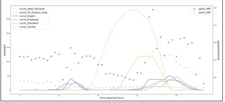
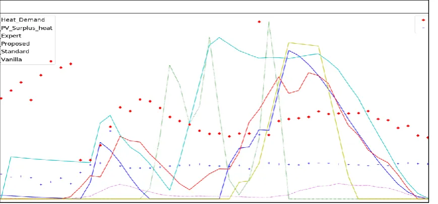
Showed in Figure 5.2, the Standard Model and the Proposed Model exhibit a similar behaviour of the expert. Both Models identified the two demand peaks in the morning and the evening. It is obvious that the Vanilla Model has no ability to predict future heat demand. Therefore, the Vanilla Model saved more PV generation than the evening demand and lost the income of exporting PV generation to the grid. The Vanilla Model can be improved by setting two sets of on-and-off time, one for summer and another for winter, since the averages of heat demand in summer and winter are different.

We can conclude that accurate predictions of heat demand are crucial to the operation of heat storage. Figure 5.3 shows one example that the Standard Model incorrectly predicts two demand peaks. Consequently, it prepared more heat than the actual need. The excess use of heat storage in the morning leads to extra import of electricity. Another excess use in the evening consumes PV generation unnecessarily.

expects a low SBP at 𝑡₃; accordingly, the Standard Model starts to charge the heat storage too early, hence unnecessary heat loss in the heat storage occurred and, more importantly, the Standard Model imports electricity with a relative high SBP at 𝑡₃, as showed in Figure 5.4 in which the SBP (red dot) at 𝑡₃ (approx. 0.048 £/kWh) is much higher than 𝑡₁₀ (approx. 0.036 £/kWh), of which time the expert starts to charge the storage in the morning.

The same behaviour of the Standard Model can be seen in Figure 5.5 during the morning. Since outputs of the unreliable SBP predictor in the Standard Model are stuck around the average of SBPs, it’s hard for the Standard Model to detect the sudden drop of SBP at 𝑡₁₀

in Figure 5.5.

In addition, incorrect prediction of PV generation can also weaken the performance of the Standard Model. In Figure 5.4, there are two PV generation peaks at 𝑡₂₃, and 𝑡₂₉. Unlike the Proposed Model and the expert, the Standard Model charges no heat into the storage during the peak at 𝑡29 because it does not expect this PV generation peak. It uses PV generation peak at 𝑡₂₃ to charge the storage, and hence suffers from unnecessary heat loss in the heat storage.

Chapter 5 Results and Discussion

The operation curve of the Proposed Model demonstrates roughly the same pattern as of the expert. Unlike the Standard Model, the network in the Proposed Model is trained to directly predict a target level. We cannot discuss the behaviour of the Proposed Model like we do with the Standard Model in above paragraphs because the network in the Proposed Model does not predict each feature separately.

Figure 5.2 One-day simulation (Result 1)

Figure 5.3 One-day simulation (Result 2)

Chapter 5 Results and Discussion

Figure 5.5 One-day simulation (Result 4)

5.3

Annual Cost

One way to examine the performance is to compare the operation costs of each Model in simulation. We run three one-year simulations for the all the Models and summed the daily operation cost according to Equation (3). The results are showed in Table 5.1. Note that the last Model in the table has no heat storage. It sells all PV Surplus to the grid, and whenever there is a Shortage, it imports electricity.

Negative operation cost indicates that the system exported more electricity than imported from the grid in a year. Model without storage has the highest income of importing electricity in all three simulations, as showed in Column (A) in Table 5.1.

Expenditure of importing in Equation (3) can be further separated depending on its purpose, as showed in Column (B) and (C). Since the Vanilla Model and the Model without storage cannot charging the heat storage by importing electricity, both shows zero in Column (C).

Vanilla Model fail to reduce overall operation cost, compared to the Model without heat storage.

To compare the performance of these Models, we defined a number, 𝑒_𝑜𝑝, that describes

the effectiveness of operation. Operating the heat storage, a Model decreases the total revenue of exporting electricity and increases the total expenditure of importing electricity from the grid for charging the heat storage, as showed in Equation (8) and (9). Similarly, the operation of heat storage reduces the total expenditure of importing electricity for meeting the heat demand, as Equation (10). The Models aim to decrease 𝐸𝑃𝑉+ 𝐸𝐺𝑟𝑖𝑑 and increase 𝑅 as much as possible because a higher 𝑒𝑜𝑝 indicates that a

Model profits from its operation more effectively, as Equation (11). It is profitable to implement a Model only if the 𝑒_𝑜𝑝 of that Model is larger than 1.

𝑬𝑷𝑽= 𝑬𝒙𝒑𝒆𝒏𝒅𝒊𝒕𝒖𝒓𝒆 𝒐𝒇 𝑷𝑽 𝑺𝒖𝒓𝒑𝒍𝒖𝒔 𝒇𝒐𝒓 𝒄𝒉𝒂𝒓𝒈𝒊𝒏𝒈 𝒕𝒉𝒆 𝒔𝒕𝒐𝒓𝒂𝒈𝒆

= (𝑹𝒆𝒗𝒆𝒏𝒖𝒆 𝒐𝒇 𝒂 𝑴𝒐𝒅𝒆𝒍) − (𝑹𝒆𝒗𝒆𝒏𝒖𝒆 𝒐𝒇 𝒕𝒉𝒆 𝑴𝒐𝒅𝒆𝒍 𝒘𝒊𝒕𝒉𝒐𝒖𝒕 𝒔𝒕𝒐𝒓𝒂𝒈𝒆)

( 8 )

𝑬𝑮𝒓𝒊𝒅= 𝑬𝒙𝒑𝒆𝒏𝒅𝒊𝒕𝒖𝒓𝒆 𝒐𝒇 𝒊𝒎𝒑𝒐𝒓𝒕𝒊𝒏𝒈 𝒆𝒍𝒆𝒄𝒕𝒓𝒊𝒄𝒊𝒕𝒚 𝒇𝒐𝒓 𝒄𝒉𝒂𝒓𝒈𝒊𝒏𝒈 𝒕𝒉𝒆 𝒔𝒕𝒐𝒓𝒂𝒈𝒆

( 9 )

𝑹 = 𝑹𝒆𝒅𝒖𝒄𝒕𝒊𝒐𝒏 𝒊𝒏 𝑬𝒙𝒑𝒆𝒏𝒅𝒊𝒕𝒖𝒓𝒆 𝒐𝒇 𝒊𝒎𝒑𝒐𝒓𝒕𝒊𝒏𝒈 𝒆𝒍𝒆𝒄𝒕𝒓𝒊𝒄𝒊𝒕𝒚 𝒇𝒐𝒓 𝒉𝒆𝒂𝒕 𝒅𝒆𝒎𝒂𝒏𝒅

= (𝑬𝒙𝒑𝒆𝒏𝒅𝒊𝒕𝒖𝒓𝒆 𝒐𝒇 𝒕𝒉𝒆 𝑴𝒐𝒅𝒆𝒍 𝒘𝒊𝒕𝒉𝒐𝒖𝒕 𝒔𝒕𝒐𝒓𝒂𝒈𝒆) − (𝑬𝒙𝒑𝒆𝒏𝒅𝒊𝒕𝒖𝒓𝒆 𝒐𝒇 𝒂 𝑴𝒐𝒅𝒆𝒍) ( 10 )

𝒆𝒐𝒑= 𝑹

𝑬𝑷𝑽+𝑬𝑮𝒓𝒊𝒅 ( 11 )

Table 5.2 shows each 𝑒_𝑜𝑝 of each Model in the three simulations. As the same we observe

from the comparison of total operation cost of each Model, the expert has the highest 𝑒𝑜𝑝 around 1.55. Our Propose Model nearly meets the requirement with a 𝑒𝑜𝑝 around 0.98.

Chapter 5 Results and Discussion

We also calculated different 𝑒_𝑜𝑝 in each week in the simulation result 1, as showed in

Table 5.3, to examine how PV generation and heat demand affects 𝑒𝑜𝑝 of each Model.

During the cold weeks, such as week 1, 2, 12 and 13, we have smaller amount of PV generation to meet the heat demand directly or to be charged into the heat storage in advanced. Since SBP are always larger or equal to SSP, using PV Surplus is usually more economical than importing electricity. Consequently, with less amount of economical PV generation, the operation costs of these weeks are positive.

It should be note that the term, ‘cold’ or ‘warm,’ does not mean that the weather is colder or warmer in those weeks. ‘Cold’ means the system must import more electricity from the grid because the total PV generation is relative lower, and/or the total heat demand is relative higher.

The 𝑒𝑜𝑝 of the Proposed Model, Standard Model and Vanilla Model is greater than 1 during the cold weeks. In addition, 𝑒_𝑜𝑝 of the expert during the cold weeks are greater

than during the warm weeks. This is because most of the time during the cold weeks the Models has no need to predict PV generation correctly since PV generation in cold weeks is relative less and has less influence on operation. Consequently, the Models need only reliable predictions on demand and prices, and thus it is easier for the Models to make a better decision. Since the price predictors of the Standard Model are less effective, the 𝑒_𝑜𝑝 of the Standard Model is lower than of others in the cold weeks.

The Vanilla Model sometimes has better 𝑒𝑜𝑝 during cold weeks because most of the time

Note that even though the 𝑒_𝑜𝑝 of the Vanilla Model is greater, it does not guarantee that

the Vanilla Model can outperform other Models because the Vanilla Model has no concern with price prediction and importing electricity. Table 5.4 shows the 𝑒_𝑜𝑝 and the total reduction, 𝑅, of operation cost during cold weeks. In week 1, the 𝑒_𝑜𝑝 of the Vanilla

Model (1.54) is greater than the Proposed Model (1.32). However, 𝑅 of the Vanilla Model (£65) is less than the Proposed Model (£197). The same occurs in week 13.

Table 5.1 Yearly Operation Cost

Result 1:

Model

(D)

Operation Cost (£)

(D)=(A)+(B)+(C)

(A)

Sell to the

Grid

(B)

Buy for Heat

Demand

(C)

Buy for

Charging

Expert -48999 -53150 1494 2657

Proposed Model -46429 -53377 3889 3059

Standard Model -44744 -52577 3212 4621

Vanilla Model -44433 -51245 6812 0

Chapter 5 Results and Discussion

Result 2:

Model

Operation Cost (£)

(A)+(B)+(C)

(A)

Sell to the

Grid

(B)

Buy for Heat

Demand

(C)

Buy for

Charging

Expert -51713 -55934 1428 2793

Proposed Model -49154 -56131 3763 3214

Standard Model -47452 -55345 3144 4749

Vanilla Model -47151 -54062 6911 0

Without Storage -49272 -57608 8336 0

Result 3:

Model

Operation Cost (£)

(A)+(B)+(C)

(A)

Sell to the

Grid

(B)

Buy for Heat

Demand

(C)

Buy for

Charging

Expert -42620 -46884 1619 2645

Proposed Model -40072 -47185 4103 3010

Standard Model -38491 -46326 3325 4510

Vanilla Model -38236 -45116 6880 0

Table 5.2 Operation effectiveness, 𝒆𝒐𝒑

Model Result 1 Result 2 Result 3

Expert 1.57 1.55 1.54

Proposed Model 0.99 0.97 0.97

Standard Model 0.75 0.74 0.75

Vanilla Model 0.45 0.40 0.44

Table 5.3 Operation effectiveness, 𝒆_𝒐𝒑, of each week in Result 1

Week Expert

Proposed Model Standard Model Vanilla Model Operation Cost

1 1.74 1.32 1.16 1.54 positive

2 1.6 1.16 0.99 1.47 positive

3 1.43 0.89 0.75 0.77 negative

4 1.43 0.71 0.58 0.31 negative

5 1.42 0.68 0.47 0.12 negative

Chapter 5 Results and Discussion

Week Expert

Proposed Model Standard Model Vanilla Model Operation Cost

7 1.46 0.36 0.26 0.05 negative

8 1.56 0.46 0.39 0.06 negative

9 1.43 0.65 0.49 0.13 negative

10 1.46 0.81 0.62 0.29 negative

11 1.45 0.85 0.75 0.49 negative

12 1.59 1.19 1.01 1.01 positive

13 1.72 1.27 1.06 1.50 positive

Table 5.4𝒆_𝒐𝒑 and 𝑹 of operation cost during cold weeks in Result 1

Expert Proposed Model Standard Model Vanilla Model Week 1

𝑒_𝑜𝑝 1.74 1.32 1.16 1.54

Expert Proposed Model Standard Model Vanilla Model Week 2

𝑒𝑜𝑝 1.6 1.16 0.99 1.47

𝑅 379 90 -7 103

Week 12

𝑒_𝑜𝑝 1.59 1.19 1.01 1.01

𝑅 363 113 7 2

Week 13

𝑒𝑜𝑝 1.72 1.27 1.06 1.50

𝑅 440 169 46 63

5.4

Training and Computation Efficiency

Since the Standard Model and the Proposed Model follow the different concept as showed in Figure 1.1, Figure 1.2, Figure 1.3 and Figure 1.4, it is interesting to examine the training and computation efficiency of the two Models.

5.4.1

Preparation of Training Dataset

Chapter 5 Results and Discussion

the contrary, it took approx. 6 hours to prepare the dataset for the Proposed Model due to the computation caused by running Algorithm 1 for a four-year historical data.

5.4.2

Training of Models

It is meaningless to compare the training time of each LSTM networks because the total number of trainable weights/varaiables is different in different Model. In addition, the training time can also be influenced by the complexity of the dataset, which is different for each predictor.

5.4.3

Computation Efficiency

6

Conclusion

In this paper we proposed a LSTM model for the operation of heat storage in a solar energy community distribution system with PV generation as the only domestic generation and a connection to the main grid. Unlike conventional LSTM model that the networks are only used to predict features for supporting an operator or a control programme to make a decision, our proposed model integrates the operation strategy into the network, and thus provide an operation action directly.

With historical data, we created an expert who can perfectly predict future. This expert follows the operation strategy we proposed in this paper, and then the operation behaviours of this expert are used to train a LSTM network in our proposed model.

We set up three different Models:

A. The Standard Model has five LSTM networks that receive past values of PV generation, electricity demand, heat demand, SSP and SBP to predict future values. These predictive values are then passed to a control programme that follows the operation strategy proposed in this paper to calculate the current target level of the heat storage.

B. The Proposed Model has only one LSTM network that is trained by the operation behaviour of the mock-up expert. This network receives past values of PV generation, electricity demand, heat demand, SSP and SBP to provide the current target level of the heat storage.

Chapter 6 Conclusion

We conducted one-year simulations for the expert, the three Models and a system without heat storage. To decrease the total cost of importing electricity to meet the heat demand, each model consumes PV generation that could have been sold to the grid or imports electricity to charge the heat storage when SBP is relative low. We defined a number, 𝑒𝑜𝑝,

to describe the operation effectiveness of a Model:

𝒆𝒐𝒑= 𝑹 𝑬𝑷𝑽+𝑬𝑮𝒓𝒊𝒅

𝑹 = 𝑹𝒆𝒅𝒖𝒄𝒕𝒊𝒐𝒏 𝒊𝒏 𝑬𝒙𝒑𝒆𝒏𝒅𝒊𝒕𝒖𝒓𝒆 𝒐𝒇 𝒊𝒎𝒑𝒐𝒓𝒕𝒊𝒏𝒈 𝒆𝒍𝒆𝒄𝒕𝒓𝒊𝒄𝒊𝒕𝒚 𝒇𝒐𝒓 𝒉𝒆𝒂𝒕 𝒅𝒆𝒎𝒂𝒏𝒅

𝑬 = 𝑬𝒙𝒑𝒆𝒏𝒅𝒊𝒕𝒖𝒓𝒆 𝒐𝒇 𝑷𝑽 𝑺𝒖𝒓𝒑𝒍𝒖𝒔 𝒐𝒓 𝒊𝒎𝒑𝒐𝒓𝒕𝒊𝒏𝒈 𝒆𝒍𝒆𝒄𝒕𝒓𝒊𝒄𝒊𝒕𝒚 𝒇𝒐𝒓 𝒄𝒉𝒂𝒓𝒈𝒊𝒏𝒈 𝒉𝒆𝒂𝒕 𝒔𝒕𝒐𝒓𝒂𝒈𝒆

The results of one-year simulations show that the expert has the highest 𝑒_𝑜𝑝 around 1.55, and the Propose Model has 𝑒_𝑜𝑝 around 0.98. The Standard Model and the Vanilla Model

fails with 𝑒𝑜𝑝 around 0.75 and 0.45 respectively. The performance of our Proposed Model is nearly to be profitable if its 𝑒_𝑜𝑝 can be further improved to be greater than 1.

We found that during the weeks when the PV generation is low, and the heat demand is high, the 𝑒𝑜𝑝 of the Proposed Model, Standard Model and Vanilla Model is greater than

1. This is because the accuracy of prediction on PV generation has less influence on the performance of a Model. Thus, it is easier for a Model to operate the heat storage during a ‘colder’ week.

With the same input (five features at 𝑡_𝑛−48 to 𝑡_𝑛−1), our Proposed Model has a better operation efficiency and less computation time in simulation than the Standard Model that follows the conventional way of implement LSTM networks in decision making of system operation.

In further studies, we intend to create other experts by new operation strategies or by real experience of human operator. By introducing new operation strategy, the number of input features may increase or decrease and further affect 𝑒𝑜𝑝 of the model. On the other

hand, if we introduce human operation experience, the selection of input features would be the key decision for constructing the model. Alternatively, the model can learn directly from extracting a policy from the human operation experience [11] without conducting a supervised learning.

We also aim to examine different scenario for this solar energy community distribution system, such as an increase or decrease in the number of houses or solar panels. This would affect 𝑒𝑜𝑝 of the models because it changes the amount of PV generation and heat

Chapter 7 References

7

References

[1] Hochreiter, S., & Schmidhuber, J. (1997). Long short-term memory. Neural computation, 9(8), 1735-1780.

[2] Rahman, A., Srikumar, V., & Smith, A. D. (2018). Predicting electricity consumption for commercial and residential buildings using deep recurrent neural networks. Applied Energy, 212, 372-385.

[3] Marino, D. L., Amarasinghe, K., & Manic, M. (2016, October). Building energy load forecasting using deep neural networks. In Industrial Electronics Society, IECON 2016-42nd Annual Conference of the IEEE (pp. 7046-7051). IEEE.

[4] Zaytar, M. A., & El Amrani, C. (2016). Sequence to sequence weather forecasting with long short term memory recurrent neural networks. Int J Comput Appl, 143(11). [5] Qing, X., & Niu, Y. (2018). Hourly day-ahead solar irradiance prediction using

weather forecasts by LSTM. Energy, 148, 461-468.

[6] Mellit, A., & Pavan, A. M. (2010). A 24-h forecast of solar irradiance using artificial neural network: Application for performance prediction of a grid-connected PV plant at Trieste, Italy. Solar Energy, 84(5), 807-821.

[7] Chu, W. T., Ho, K. C., & Borji, A. (2018). Visual Weather Temperature Prediction. arXiv preprint arXiv:1801.08267.

[9] Zhang, D., Martinez, N., Lindholm, G., & Ratnaweera, H. (2018). Manage Sewer In-Line Storage Control Using Hydraulic Model and Recurrent Neural Network. Water Resources Management, 32(6), 2079-2098.

[10] Chollet, F. (2015). Keras. https://keras.io/

Chapter 8 Appendices

8

Appendices

Appendix 1 Comparisons of predictive and true values in the Standard Model 48

Appendix 1 Comparisons of predictive and true values

in the Standard Model