THE MAXIMUM PRINCIPLE, ITS COMPUTATIONAL ASPECTS AND ITS RELATIONS TO OTHER OPTIMIZATION TECHNIQUES EUR 590 e

jiUH!«ä;t'5L.saaiwsi

i

i

n

inp

SUR

■

■ : THE MAXIMUM PRINCIPLE, ITS S i i l i

MPUTATIONAL ASPECTS AND ITS RELATIONS

This document was prepared under the sponsorship of the Commission of

the European Atomic Energy Community (EURATOM).

Neither the EURATOM Commission, its contractors nor any person acting

on their behalf :

1° — Make any warranty or representation, express or implied, with respect to the

accuracy, completeness, or usefulness of the information contained in this

document, or that the use of any information, apparatus, method, or process

disclosed in this document may not infringe privately owned rights ; or

^ M f C S ( M Ì E

EUR 590.e

THE MAXIMUM PEINCIPLE, ITS COMPUTATIONAL ASPECTS AND ITS RELATIONS TO OTHER OPTIMIZATION TECHNIQUES by W. DE BACKER

European Atomic Energy Community — EURATOM

Joint Nuclear Research Center — Ispra Establishment (Italy) Scientific Data Processing Center — CETIS

Brussels, February 1964 — 75 pages — 3 figures

This report is the text of an introductory seminar held in April 1963 on the theory of optimal processes. The maximum principle of Pontryagin and its relations to the principle of opti-mality of Bellman, the classical calculus of variations and gradient methods (generalized gradient) are discussed. The computational aspects of the synthesis of optimal systems on electronic computers are analyzed, especially those connected with the theory of penalty functions, the two-point boundary problem, parameter optimization and sensitivity analysis. The need of hybrid computation is under-lined.

EUR 590.e

THE MAXIMUM PRINCIPLE, ITS COMPUTATIONAL ASPECTS AND ITS RELATIONS TO OTHER OPTIMIZATION TECHNIQUES by W. DE BACKER

European Atomic Energy Community — EURATOM

Joint Nuclear Research Center — Ispra Establishment (Italy) Scientific Data Processing Center — CETIS

Brussels, February 1964 — 75 pages — 3 figures

This report is the text of an introductory seminar held in April 1963 on the theory of optimal processes. The maximum principle of Pontryagin and its relations to the principle of opti-mality of Bellman, the classical calculus of variations and gradient methods (generalized gradient) are discussed. The computational aspects of the synthesis of optimal systems on electronic computers are analyzed, especially those connected with the theory of penalty functions, the two-point boundary problem, parameter optimization and sensitivity analysis. The need of hybrid computation is under-lined.

EUR 590.e

THE MAXIMUM PRINCIPLE, ITS COMPUTATIONAL ASPECTS AND ITS RELATIONS TO OTHER OPTIMIZATION TECHNIQUES by W. DE BACKER

European Atomic Energy Community — EURATOM

Joint Nuclear Research Center — Ispra Establishment (Italy) Scientific Data Processing Center — CETIS

Brussels, February 1964 — 75 pages — 3 figures

EUR 590.e

EUROPEAN ATOMIC ENERGY COMMUNITY - EURATOM

THE MAXIMUM PRINCIPLE, ITS

COMPUTATIONAL ASPECTS AND ITS RELATIONS

TO OTHER OPTIMIZATION TECHNIQUES

by

W. DE BACKER

1964

Joint Nuclear Research Center Ispra Establishment - Italy

CONTENTS

Page

INTRODUCTION 7 Chapter 1 - TIIE MAXIMUM PRINCIPLE 9

1.1. Statement of the fundamental problem 9

1.2. Discussion 9 1.2.1. The system of dynamical constraints 10

1.2.2. The control variables 11 1.2.3. Restricted state variables 13

1.2.4. The functional J 13 1.2.5. Initial and final conditions 14

1.3· The maximum principle and the theorems of the Pontryagin team 15

1.3.1. The optimal trajectory lies in the interior of G 15 1.3.2. The optimal trajectory lies on the boundary of G 16 1·3·3· The optimal trajectory partly lies in the interior

of G and partly on the boundary of G 18

1. 3 · 4 · Remarks I9 1.4· The principle of optimality and its relation to the maximum

principle I9 1.4.1. The principle of optimality 19

1.4.2. The continuous version of the principle of optimality 20

1.4·3. The Hamilton!an system 21 1.4.4· Remarks ,. 22

1.5· The calculus of variations and its relation to the maximum

principle 22 1.5.1. Survey . 22

1.5·2. An example - Analytical mechanics as an optimal process .... 23

1.6, An i llustrative er: rei se . 24

Chapter 2 ­ COMPUTATIGNAL ASPECTS OF THE MAXIMIM PRINCIPLE 29

2.1. General computing diagram 29

2.2. The illustrative exercise of § 1.6 30

2.3. The χ ­'ψ­ models 31

2.4. The Lagrange multipliers 31

2.5· The maximization of ç\t 32

2.6. The two­point boundary problem 34

2.7· Dynamic programming 35

2.8. Conclusions 36

Chapter 3 ­ PENALTY FUNCTIONS 38

3.1. Introduction 38

3.2. Statement of the penalty problem 38

3.3. Formal application of the maximum principle to the

penalty problem 39

3.4· A second version of the penalty problem 40

3· 5· Discussion 41

3.6. Computational aspects 42

3.7· Example 44

3.8. Conclusions 47

Chapter 4 ­ THE GENERALIZED GRADIENT 48

4. 1 · Introduction 48

4.2. Statement of the problem 49

4­3. The generalized gradient as a special case of the

maximum principle 5O

4.3.1. The optimal trajectory lies in the interior of G 50 4.3.2. The trajectory partly lies in the interior of G

and. partly on the boundary of G 51

4.3.3. The transversality conditions 52

4.3.4. Conclusions 53

4.4. The steepest descent as a special case of the generalized

gradient 55

4.5· Computational aspects of the generalized gradient 56 4.6. Example of a generalized gradient application 57

Chapter 5 - TWO-POINT BOUNDARY PROBLELIS AND PARAMETER OPTIMIZATION ... 60

5.1. Introduction 60 5.2. The two-point boundary problem as an optimization problem 60

5.3. Sensitivity equations 62 5.4. Parameter Optimization 64 5.5. General discussion and computational aspects 65

5.5·1· Convergence problems 65 5.5.2. Local and global optima 66 5.5·3. Sensitivity and discontinuity problems 67

5·5·4· Iterative analog computers 68 5.6. The illustrative exercise of § 1.6. and § 2.2 69

7

-INTRODUCTION

This report is the text of an introductory seminar on optimal control held by the author for EURATOM personnel at CETIS in April I963.

after the first IFAC-Congress held in Moscow in I960, a growing interest in optimal control has been noticed throughout the world. Many contri-butions in this field originated in some very important papers presented at the congress, especially those by Pontryagin, Bellman and their

respective co-authors.

In this report we are concerned with the mathematical theory developed by the Pontryagin team and which is better known as the Maximum Principle. As an introduction we tried to give a synthetic statement of the theorems on the Maximum Principle and to discuss its relations to other optimization techniques (chapters 1 and 3)· Our main point of interest however is the synthesis of optimal control and particularly its computational aspects. As, as yet this is an unsolved problem we tried to give a general outline of present possibilities and future hopes (chapters 2, 3 and 5)· Some original work of the author on penalty functions and generalized gradient techniques has been included (cfr. chapter 3 and 4)·

However, since progress is very quick in this field new important develop-ments have been published after April 1963· This was particxilarly the case at the second IFAC-Congress held in Basle in September 1963, where optimal control was the main topic in the theoretical section. Some problems we referred to in this report are already solved now, for instance the synthesis of linear optimal control and some theoretical difficulties in connection with penalty functions.

­ 9 ­

CHAPTER 1 THE MAXIMUM PRINCIPLE

1.1. Statement of the fundamental Problem

Ne consider χ (t) to be the state vector χ (t) = (χ (t), . . ., χ (t), . . ., χ ( t ) ) , belonging to a region G of the n­dimen­ sional state space and whose evolution is described by a system of differential equations

¿ 2 $ Û . . f [ χ (t), u ( t ) J

( 1 )

1 vi * Ί

with f = ( f , . . . , f ) . In t h i s system u ( t ) = ( u ( t ) , . . . , u ( t ) ) i s a c o n t r o l v e c t o r whose range i s i n a subset U of the

r-dimensional c o n t r o l space. The subset U i s u s u a l l y defined hy

q1 (u) S 0 1 = . 1 , . . . , s ( 2 )

and the region G i s u s u a l l y defined by

gJ U ) ζ 0 j = 1, . . . , m ( 3 )

In relations ( 2 ) and ( 3 ) the inequality sign is optional.

The initial condition χ (t ) = χ and the final condition χ (t,) =

v o' o 1

χ of the system belong respectively to the sets S and S which are smooth manifolds in G of arbitrary dimension (but less than n), Among all admissible controls u£U which transfer the point χ from

χ £S to x„£S„, it is asked to find one for which the functional _o

c o 1 1 '

J = *

J f°[ χ (t), u (t)j dt ( 4 )

o

takes on the least possible value.

1.2. Discussion

10

1.2.1. The system of dynamical constraints

The set of equations ( 1 ) covers a very general class of dynamical systems and probably is the most general one which is possible to program on an analog computer. It consists of n different first order differential equations of the type

dx _ i / 1 2 i n 1 r\

*j , — 1 ^ JL. · -Χ. J · · » j Jv ρ « * « y jL t) LX ^ · · · j U. J

It can easily be shown that an η­order differential equation can be written as a set of η first order differential equations.

2

Example t χ + ¿~Ύ ¿o χ + ¿O x = c is equivalent to

dx" 0<v, 2 , , 2 1

•TT— = c ­_{dt ^-S o o} ¿Ύον x -Cc) χ

dx1 2

χ

dt

2 · 1 with χ = χ and χ = χ

It should be remembered that even a partial differential equation corresponds to the formulation ( 1 ), but then with η = 00. The approximation by finite differences however, which is a common technique for solving partial differential

equations on analog and digital computers, automatically fits in with ( 1 ) since η has been given a finite number.

The vector equation ( 1 ) itself may be the subject of a finite difference approximation with respect to time

χ (t

+ΔΙ)

= χ (t) + f [χ (t), u (t)]

¿¡t

( 5 )

or

i Λ t 1 η 1 Γ\ Γ / ν

χ = χ + f (χ , . . . , χ , u , . . ., u )ò ( 5 )

J ' J J J J J

with S = ¿t

j = 1 , . . . , Ν

11

The set ( 1 ) generally represents the model of a dynamical system such as a space engine, a nuclear reactor or a power generating system. We would draw attention to the importance of the simplicity and validity of such a model with respect to the physical system. Without simplicity and especially without a reasonably low number of equations the optimization,

even with large electronic computers, becomes a heavy, risky and even an impossible task. On the other hand a lack of knowledge about the validity and the regions of validity of

a simplified model may lead to solutions which are completely unrealistic from a physical point of view.

1.2.2. The control variables

The essential difference between the state variables and the control variables is that the latter are completely free from dynamical constraints. At every instant they can be chosen anywhere in the control region U.

If some variable, subject of a dynamical constraint were considered as a control variable, the optimization would take place ignoring that constraint. This generally gives rise to surprising and very unrealistic results. It may be dangerous, for instance, to ignore the inertia and the trans­

fer function of the control system itself, even if at first sight its quality would suggest their unimportance. This again points out the problem of the validity of the dynami­ cal model.

For the mathematical statement of the problem,U could be an arbitrary set, but in technical problems U is always a closed set. Some particular types of control regions are

- the hypercube q (u) = J u j - 1 £ 0 ( 6 )

i = 1 , . . . , n

Ή

- the hypersphere q (u) = ^""(u1) - 1 = (u, u) - 1 < 0 ) (7)

The number of control variables r, especially when compared with η, is evidently a very important characteristic of the

control possibilities of the system.

12

In some problems time appears explicitly in f (χ, u, t ) , f (χ, u, t) or g (χ, t ) , making the whole system non­ autonomous. In such a case we consider time as a new state variable χ = t wherever it appears explicitly, while a new differential equation dx /dt = 1 is added to the system. In this way we obviously satisfy once more the ge­ neral definition of ( 1 ) .

Algebraic relations between state variables of the type l~P(x) = 0 are more difficult to handle. In most cases Φ (χ) = 0 can be solved for one state variable as a function

of the others χ = θ (χ , . . ., χ , χ , , . , , χ ) ,

i Of

which can be introduced in all f wherever χ appears. Such a substition is surely the "cleanest" method. Sometimes how­ ever this technique is not desirable because of programming difficulties. This is particularly true if several nonlinear algebraic relations have to be treated. Therefore a second

possibility is to consider Ψ ( χ ) = 0 as a relation of type ( 3 )> for which Lagrange multipliers have to be introduced, as will be shown by the theorems of Pontryagin.

Sometimes no system of dynamical constraints has been given, but the time derivative χ of the state variable χ has to be chosen in order to minimize the given functional. In this case it should not be forgotten that system ( 1 ) takes the form

dx ι .

T T ­ = u ι = 1, . . ., η

Although equations of the type dx „

dt

Γχ (t), χ ( t - ^ ) , χ (t -r

), . . ., u (t)]

- 13

1.2.3. Restricted state variables

The control vector u£U has to be chosen such that χ stays

in the interior of G. We already know from ( 3 ) that G may

be defined by inequality or equality constraints. We also

noticed that the last case offers the possibility of in­

troducing algebraic relations of the type^P(x) » 0.

Sometimes additional equations of type (· 1 ) are necessary

for the definition of G. We take the example of integral

constraints;

t

O (x,uj dt' < A

ƒ,

t

_o

Then we introduce the a d d i t i o n a l equation

η + 1

dx _ η + 1 / \ _ / \

¿ t — = f

( χ , u) = D ( x , u)

n + 1

such that G can be defined by χ

­ A ^ 0.

According to the application, g (χ) may be the maximum

altitude of an aircraft, a mechanical stop in a servo­

mechanism, the maximum operating temperature of an electric

motor, a given disposable income budget or an integral con­

straint such as the charge of an accumulator or an available

quantity of fuel.

1.2.4. The functional J

Introducing the definition

^ t

= f ° [ x ( t ) , u(t)]

with x° (t

) = x°

( 8 )

we see that J = x. ­ χ and the problem reduces to finding

u (t) such that χ (t.) takes on the least possible value.

Every maximal problem can be changed into a minimal problem

by inverting the sign of f (χ, u).

Equation ( 8 ) can be

added to the set of equations ( 1 ) increasing the order

of the system by one. It has to be observed, however, that

14 ­

Some special cases are of particular interest. Taking f° (x, u) = 1 we have J = t ­ t , representing a time­ optimal problem. This already shows that neither t nor t. necessarily has to be given by the problem. They can be part of the solution. It may equally happen that J o F (χ.) ­ F (χ ) is a function only of the initial and final conditions of the state variables, which implies f° (x, u) = dF/dt = ("ì>F/t>x, f ) . Both cases will be studied later (cfr. § 1.7. and chapter 4 ) .

Some authors prefer the expression f (χ, χ, t ) . It can easily be shown that this is a special case of our defi­ nition f (χ, u ) . We only have to consider t as a new

state variable (cfr. § 1.2.1.) and to substitute all χ by the corresponding f (χ, u) of the equations ( 1 ) . The right definition of the optimization criterion is of

course the crucial point of the problem. It can be the mean square error in a servomechanism, the consumption

of fuel of a missile or an aircraft, some maximal distance, minimal time, minimal cost in a production process, mini­ mal xenon poisoning during the shutdown of a nuclear reactor, etc.

Finally, it may happen that the function f (χ, u) is not given explicitly, but has to be measured while optimizing. This new restriction imposes special techniques, which will not be discussed.

I.2.5. Initial and final conditions

The fact that S and S. are sets implies that χ and x_

o 1 * . o 1

15 ­

An interesting case is where every instant t is considered as a t of an optimization process ending at t = t + T. .After having solved the problem for t 4 t'4 t + T, the

initial decision u (t) is taken and this brings the system to the time t +¿Jt where the whole optimization process has to be repeated for t = t +At. In this way we have a continuous sequence of optimization processes of which the initial decisions describe a time trajectory. Some aspects of this problem are studied in chapter 4·

1.3. The Maximum Principle and the Theorems of the Pontryagin Team We shall restrict ourselves to a very condensed statement of the theorems concerning the maximum principle. For more mathematical details as well as rigorous demonstrations we refer to ref. £ l j . Three cases have to be distinguished.

1.3.1. The optimal trajectory lies in the interior of G

We assume the functions f (x, u) (i = 0, 1, ..., η) to be defined and continuous together with their partial deri­ vatives'^ /£>x , of= 1, ..., n, on G χ U. Admissible

controls u (t)éU have to be piecewise continuous.

In order to formulate the maximum principle we consider in addition to the system ( 1 ) another set of differential equations in the continuous non­zero variables /»/!!> ···>

Γ , called the adjoint system..

η

dt -

- 2 _

-τ,

J.

i

i = 0, 1, ... , η Introducing the definition

de&,

χ, u)

=Y^f

(χ,

u)

( 10 )

16

-d^-H i- 0,1....,» (11)

— 1 - r i - O, 1, ... , η (12)

dt

dx

Theorem:

Necessary conditions for optimality of the problem

stated in § 1.1., with the above mentioned restrictions and

definitions, are

1. Maximum condition

At every instant t , u(t) has to be chosen such that «ft

attains i t s leaet upper bound

7Τ6(ψ, χ) - aup # ( ψ , χ, u) (13)

u 6 U

2. Terminal conditions

%(^)¿0

TTCpftt,), xC^)]­ 0

(14)

3. Transversality conditions

T|T(t

) has to

be orthogonal to

a tangent plane of

S

in

the point

€· S

·

"^(t.) has to

be orthogonal to

a tangent plane of S. in

the point x.€S .

*

If these three conditions are satisfied it results that iJT­

is constant and

ud( γ

,x) =■

0 at any time t, t _ ¿ t ¿ t

,

and not just at t..

Whenever ψ

is

different from zero, which is true for

nearly all possible applications, we can take ψ

« ­1,

since the

adjoint system (9) is

homogeneous in

ψ .

1.3.2. The optimal trajectory lies on the boundary of G

Necessary conditions are piecewise smooth boundaries for

U and

G, while u(t) itself has to

be

a pieoewise smooth

­ 17

We shall formulate the optimizing conditions for G and U

defined respectively by g (χ) £ 0 and q (u) £ 0 instead of

the set of relations ( 2 ) and ( 3 ). The theorems, however,

can easily be generalized for values of m and 1 bigger than

one.

Let us introduce the notations

ρ (x, u)

=?-^

, f (x, u) )

( 15 )

m

__yljLlA

*

,

For an optimal trajectory lying entirely on the boundary

g (χ) it is obviously necessary and sufficient that g (x ) = 0

and ρ (x, u) = 0 for t < t <. t..

The approach is now to introduce Lagrange· multipliers Λ (t)

and "y

(t) for g (x) and q (u) and to apply the maximum

principle as stated in § 1.2.1. Because of the Lagrange

multipliers the maximization of <^then has to be changed

into relation ( 18 ), linked to additional conditions indi­

cated below.

Theorem )

Necessary c o n d i t i o n s for o p t i m a l i t y of t h e

problem s t a t e d i n § 1 . 1 . with the r e s t r i c t i o n s of § 3 · 2 . 1 .

and § 3 - 2 . 2 . and with the d e f i n i t i o n s ( 10 ) , ( 11 ) and

( 15 ) a r e :

Dr}

¿>x

d t

- " - v

i

^ - Γ - \

i = 0, 1, . . . , η

( 16 )

) The theorem is only true for "regular" optimal trajectories. The

rigorous definition and the discussion of this requirement would

lead us too far from a synthetic statement of the theorem. For

18

-p(x,u) - O

and

g(x

) - 0

(17)

Ü A - λ

* + ^

«

j « 1 , . . . , r

(18)

9 u

9 u

9 u

ΤΤΧ(ψ,χ) - S ( l f , x , u ) - 0

(19)

ψ

( ΐ ) - constant

¿ 0

(20)

ψ" C O

i s different from zero and a tangent to the boundary

g ( x ) , whioh generally means

[ i | i ( t

) , grad g ( x ) ] - 0

(21)

This condition is only necessary in order to eliminate trivial solutions of the type "di + \2 grad g ( "p is arbi­ trary)

if d A / d t exists, (dA/dt) grad g(x) is directed towards

the interior of G or else in zero. (22) 1.3.3. The optimal trajectory partly lies in the interior of G and part­

ly on the boundary of G

For parts of the optimal trajectory in the interior of G the con­ ditions of § 1.3.1. are valid. For parts of the optimal trajeotory on the boundary of G, the conditions of § 1.3.2. have to be appliedo As yet missing is a junction condition, which every pair of adjoin­ ing sections satisfies. This condition is oalled a jump condition for the vector y(t) at the junction time Τ .

Without going into details we point out two important possibilities» a) The trajectory reaches and then follows the boundary of G. The

vector l}f(t) changes discontinuously with an amount Ugrad g(x) such that (21 ) can be satisfied.

b) The trajectory lies on the boundary of G and leaves it for the interior. No change is imposed on "ψ (t ) .

19

-1.3·4· Remarks

The theorems of Pontryagin only give necessary conditions for optimal control. Nothing is said about the existence and the uniqueness of the solution.

A straightforward application of the theorems can give serious computational complications in connection with the calculation of the Lagrange multipliers and the cri­ terion indicating the instant when the trajectory has to leave the boundary for the interior.

For this reason we refer to the technique of implicit com­ puting of Lagrange multipliers. This technique only approxi­ mates to the solution of the problem, but has the advan­

tage of bypassing a lot of complications which for this reason have not even been mentioned in the preceding para­ graphs. The technique of implicit computing of Lagrange

multipliers is related to the theory of the penalty functions which will be discussed in chapter 3·

1.4· The Principle of Optimality and its Relation to the Maximum Principle

It is our aim to show in a formal way how the maximum principle could be deduced from the principle of optimality of Bellman

(cfr. [3] PP. 56 - 59 and (j] pp. 69 - 73).

1.4·1· The principle of optimality

"An optimal policy has the property that whatever the initial state and the initial decision are, the remaining decisions must constitute an optimal policy with regard to the state resulting from the first decision" (Bellman).

This means that whatever be the initial state (all χ and not only χ ) the first decision (u (t) and not only u (t ) )

20

-Ή.<

Fig. .1.1.

The principle of optimality has been, given a discrete-time formulation and applying it to our problem of §. 1.1. we have to take the finite difference version of the time derivatives (cfr. relation ( 5 ) )

J (x) = ^ [ - f ° (x, u ) 4 t + J (x + f (x, u)4t)] ( 23 )

In this mathematical formulation of the principle of optimality J (x) has the meaning of the minimal value of

( 4 ), corresponding to the solution of the problem of § 1.1. for a trajectory starting at χ (t) at time t with a decision u (t) and ending at time t at the point x^e S,.

1 1

1.4.2. The continuous version of the principle of optimality

In order to derive a continuous version of ( 23 ) by a limit operation, we develop J (x + f (χ, u)y4t) by a time series.

Oi -,

^i>J

7>x°<

[i^tf] ( 24 )

j Γχ + f (χ,

u)¿ti = j (χ)

+y

This operation obviously requires the existence of the partial derivatives of J with respect to all χ . Intro­ ducing ( 24 ) into ( 23 ) , cancelling J (x) in both membersj deviding all terms by Δ± and passing through the limit, we obtain

Max ufU

m

-

f° (x, u) + y ^

f^(x, u)

21 ­

Remarking that we have by definition

^>J

(x)

7i

[χ

(t-,) - x° (t)l _ _

n>x°

n> x°

(t)

i t i s p o s s i b l e t o w r i t e ( 25 ) a s f o l l o w s Max

uiU _^

f U ' U )

= 0

Relation ( 26 ) coincides with the maximum principle and

the relations ( 10 ), ( 13 ) and ( 14 ). The only point

which should be cleared up is the equivalence of ^ j / D x

and

γ

. In other words we want to know

If^ÒJfb

χ

as

well satisfies the Hamilton!an system.

1.4.3· The Hamilton!an system

We introduce the notations

Max

u£U

^ j

4

(Y —

f ) = M

­2>x

(x), x =

/

(χ)'­ o

( 27 )

We mean t h a t a t every i n s t a n t of the optimal t r a j e c t o r y

the maximization g i v e s a u / χ ( t ) ; , such t h a t f

(x, u)

becomes f

x, u ( x ) | = f

(x) ( s y n t h e s i s problem). I t

i s i n t h i s sense t h a t the p a r t i a l d e r i v a t i v e s

of /<?χ

have to be understood i n t h i s paragraph.

C a l c u l a t i n g -2>¿$ (x)/¿> x = 0 we hi

_lave

n>

2

Ή

« V

>'*

_ Y

Z&Ä

11

J 4

¿L

Ί>χ«

2¿

ols.t)

which i s the same a s u

Q M (JNl· x)

d_

dt

( ^ 4 )

-Ί ) χ

_{( 28 )}

At the same time we see that

"dj

dt

^»fcf

x)

22

-Equations ( 28 ) and ( 29 ) clearly constitute the Hamil-tonian system we were looking for. Moreover we identified

^ j / O x1 as the variables Τ · of the adjoint system.

1.4.4. Remarks

1. We showed how some relations of Pontryagin could be deduced from the principle of optimality of Bellman. We should not forget however that the principle of Bellman is valid for a much more general class of problems than the one we defined in § 1.1.

2. On the other hand the deduction of relation ( 26 ) was only possible on condition that J (x) was twice different­ iable. This restriction is not necessary for the theorems of Pontryagin and is not even realized for the first de­

rivative, u j/'Dx , in many current applications, parti­

cularly bang-bang problems.

3. The Hamilton!an system ( 28 ) - ( 29 ) has been formu­ lated for the already maximized M-function. This obviously makes the system unpractical for optimizing purposes since it considers u (x) as a known function.

4. The given deductions from the principle of optimality are interesting for a good understanding of the more general maximum principle. We have to keep in mind that if

^j/'O±L exists it is the same as the / . variable of the

adjoint system.

1.5. The Calculus of Variations and its Relations to the Maximum Principle

1.5.1.Survey

The problem of the calculus of variations is a particular case of the problem stated in § 1.1. The problem of Lagrange for instance is equivalent to the latter if the control region U is an open set of the r-dimensional control space E . It

χ

generally coincides with E . For this reason the maximum condition can be satisfied by relations of the type

­ 23 ­

criterion, following equally from the maximum principle for U being an open set. When U is a closed set the Weier­ strass condition is false (cfr. flj p. 256).

A still more special case is the elementary problem of Euler in the calculus of variations, corresponding to the problem of § 1.1. if f = u , G and U coinciding with the n­dimension­ al state­space and an r.­dimensional control space (r = n ) . The well­known Euler equations and the Legendre condition immediately follow from the maximum principle.

This short survey points out the importance of the maximum principle as a generalization of the classical problem of variations. This more general theory is indispensable for the very important class of applications where the optimal

trajectory corresponds to control variables partly or completely lying on the boundary of the closed control region.

1.5·2. An example ­ Analytical mechanics as an optimal process We want to derive the basic equations of mechanics in the form of an optimal trajeotoary for a Lagrange mechanical system. This problem could be solved by the calculus of variations, but we shall apply the maximum principle in order to illustrate the method. Γ 4 1

For one physical point with mass m in a potential field U (χ , Xe", χ ) the problem is characterized by

d x V d t = f1 = u1 i = 1, 2, 3 ( 3C )

3 _'i\2

,0

_2"

_{m_Ü_l}

n ( x

1

2

J = 4

It immediately follows that 3

9?- Σ ?V -Σ

SJ

P

L

+

» t*

1

■ *

2

· *

3

>

< * >

L*1 L-4

Maximization of CTT g i v e s

<~*>%

Λ / -

i

nj,

dx

= / . - m u = 0 o r r.=m -r—~

'

^ "

f«l

m τ = ­^—r (. 35 ;

­ 24 ­

Relation ( 12 ) gives

d­t ­7) l

Dx

Combining ( 33 ) and ( 34 ) we have

¿x

dt

~

Ί)

x

which is nothing else than the Newton equations for a potential field.

Finally, we want to draw attention to the meaning of ¿£ = 0

for 7= ^ÒZ/θχ in variational calculus and especially in theoretical physics. Indeed this partial differential equation corresponds to the Harailton­Jacobi equation and is connected by the Heisenberg uncertainty relations to the well­known Schrödinger equation.

It is the custom to write the partial derivative i)3/0 t explicitly in the Hamilton­Jacobi, the Schrödinger and even in the Bellman equation ( 25 ). As we considered time appearing explicitly as a state variable our relations ( 13 ) , ( 14 ) , ( 26 ) are general as well (cfr. § 1.2.1.).

1.6. An illustrative Exercise

We take the example examined in ref. jíj , p. 23, which because of its simplicity will be useful for later discussion of the computational aspects.

ρ p

We consider the equation d x/dt = u which can be rewritten in

i O

the form of the following ­system (x = χ and χ = x)

dx1 2 , , .

dt" = X ( 36 )

dx / s

- 25

The control variable u is constrained by the condition |u| ^ 1

while G coincides with the two-dimensional state space.

The problem consists of getting to the origin (θ, θ) from a

1 2

given initial state χ = (χ , χ ) in the shortest time.

t

-

o o o

The function ^L has the form

a? =f,x

_{1 ' 2}

! t

f,u-, (38)

The adjoint system is given by the equation ( 12 )

ty

= 0

2

d t

dt

y (39)

of which the solution is given by

j .

(t) = / (t ) and

%

ω .

%

(t

0

) - tY, tv

The maximization of the <3l -function gives

u = sign X

(t) ( 40 )

It follows that the control variable is a piecewise constant

function taking the values + 1 or - 1. Since ')r is a linear

time function u changes its sign only once.

Introducing relation ( 40 ) in the combined system of original

ind adjoint differential equations, the solution of the system

still depends upon the initial conditions

J\

(t ) and

[„

(t )

of the adjoint system. Considering them as parameters we have

a family of optimal trajectories, from which we have to pick out

1 °

the one which ends in the point (x = 0, xt' = θ ) . We do this by

choosing the appropriate values of

j

(t ) and /I (t ). This ii

the essence of the so-called two-point boundary problem.

Having solved the iaaximization problem and the two-point boundary

problem for ;

by Fig. 1.2.

26

-Fig. 1.2.

The optimal trajectories are composed of parts of parabolas belonging either to the family u = + 1 or the family u = - 1. Both families are separated by the switching line AOB.

1.7· Linear time-optimal Processes

The linear time-optimal problem is defined by the following equations, the meaning of which is easily understood by the discussion of the fundamental problem of § 1.1.

dx

dt = Ax + Bu ( 40 )

A and Β are l i n e a r o p e r a t o r s defined, i n terms of the c o o r d i n a t e s

1 γ\ 1 τ* "ΐ "ΐ

χ , . . . , χ and u , . . . , u , by the m a t r i c e s (a ) and ( bv) r e s p e c t i v e l y

( i = 1, . . . , n; j = 1, . . . , n; k = 1, . . . , r ) .

k;

For the time optimality we have

*i

J = 1. dt = t„ - t _{1 o ( 41 )}

t

Further, we shall assume the control region U to be a convex, closed polyhedron.

In t h i s case CA. ( / , χ, u) has the fon _)rm

-27-and the adjoint system is given by

where A is the transpose of A.

Obviously, <7L attains its maximum simultaniously with

(j,

Bu).

This implies, and it can be demonstrated, that u is piecewise

constant and that its values are vertices of U.

It can be demonstrated also (ref. Γΐj pp. 123 - 135) that the

solution of the linear time-optimal problem exists and is unique.

Up to now, such theorems have not been demonstrated for the

fundamental problem of § 1.1.

An interesting special case is where the control region U is an

r-dimensional cube

u

| έ1

■

k = 1, ..., r

( 44 )

Then we have that the maximization of

cY,

BU)

- J ; | Y ^ u

k

< « )

A­y ¿ = γ

reduces to the maximization of each of the terms

k = 1, ..., r

( 4 6 )

ce we

Σ

C*1

o b t a i n

X

k

U = !

A¿

sign

1

r

( 47 )

U-t

These results have been formulated also by La Salle f5j and

Feldbaum [6/ and they are known as the "bang­bang principle".

It follows, for instance, that if all the eigenvalues of the

matrix A are real, u has not more than η ­ 1 switchings, where

η is the order of system.

As can be verified, this confirms the results of the example of

§ 1.6. Indeed, for this second order system we have one switching

28

of u. For a third order system it would be possible to have two switching surfaces, and so on.

- 2 9 ­

Chapter 2 COMPUTATIONAL ASPECTS OF THE MAXIMUM PRINCIPLE 2.1. General Computing Diagram

One of the most important advantages of the maximum principle i3 that the particularities and special characteristics of a given optimization problem can be handled in such a way that considerable

simplification is possible with respect to the general and funda­ mental problem of § 1.1.

As a consequence, several kinds of techniques, depending on the

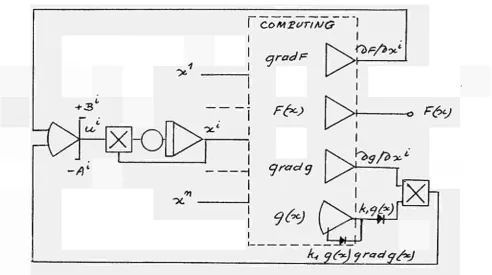
nature of the problem, can be introduced in the general optimization scheme of the Pontryagin team's theorems. Very often analytical simplifications are possible and sometimes even the solution can be found analytically. This was the case, for instance, for the example of § 1·5·2. If we are not so fortunate, computer techniques have to be tried. It is this aspect which is the object of our main interest. In order to organize our discussion about the possible simplifications and the corresponding computing techniques, we have to consider the general computing diagram (Fig. 2.1.) as it is imposed by the maximum

principle.

TWO

i

ORIGINAL SYS

oc

\

oc (t;

-POINT BOUNDARY PROBLEM

Ko

PEM

1

ujt)

1

_r

ψ)

ADJOINT SYSTEM

«¿

Ί]

1

MAXIMIZATION OF

30

The diagram comprises the original set of differential equations of the state vector χ (t), the set of differential equations of the adjoint variable j(t), a system furnishing a control vector u (t) to the systems χ and'f' such that at every instant ot ( r, x, u) has its maximum value, and finally a system which is solving the two­ point boundary problem and gives the appropriate initial conditions for the χ ­remodel.

The computational aspects of these systems will be discussed in the paragraphs following. We must not forget however that analytical simplifications can sometimes even lead to the complete elimination of one of the parts of Fig. 2.1.

2.2. The Illustrative Exercise of § 1.6.

As an illustration we could try to define the diagram of Fig. 2.1 for the optimization problem of § 1.6. , simulated on an analog computer.

TWO­POINT BOUNDARY PROBLEM

■"I

I h a s t o p u t Γ. and *C, such t h a t x . = 0 and I

1 1o ρ ¿o 1 I

31

-As we know by relation (I.40) the maximization of^t; can be simulated by a simple relay feeding the constant values + 1 or - 1 to the

x-model, depending upon the sign of γ0. The simple second order x-model

2 *" 1

has given initial conditions χ and χ , while the initial conditions 7 - and Γ of the second order adjoint system have to be calculated by the two-point boundary problem solver. Up to now the theorems of Pontryagin give no ready information about the structure of this last

system. Pontryagin himself suggests (ref. ΓΐΊ p. I81) a trial and error approach.

Of course, in the simple case of our example it is also possible to

find the solutions χ (t), χ (t), jr. (t) anåf2 (t) analytically,

and for that reason the two­point boundary problem can be solved analytically as well. The result is the synthetizing diagram of Fig. 1.2. Consequently, the computing diagram of Fig. 2.2. should be

considered only as an illustration and not as the best method for the particular case we have taken as an example.

2.3· The Original and Adjoint Systems

The computer representation of the combined χ ­ p­model poses no

new difficulties. Indeed, it consists of a set of ordinary differential equations with u = (u , ..., u ) as input variables and with initial conditions which are partially given and partially determined by the two­point boundary problem solver.

The x­model is not influenced by the f ­ variables. In general, the reverse is not true. The adjoint system is independent of the original

system only if the partial derivatives ^Of /dx do not contain χ any more. This if the case where all f are linear expressions of x. For solving ordinary differential equations analog computers are in­ dicated. For digital computers a discrete representation is necessary (cfr. ( 1.5 ) ) .

2.4. The Lagrange Multipliers

­ 32

We know by the theorems and the discussions of § 1.3.2. and '¿ 1.3­3­ that whenever the optimal trajectory reaches the boundary of G the

γ'- model has to be replaced by a new one which comprises the La­ grange multipliers for that boundary. These Lagrange multipliers have to be calculated continuously such that the trajectory moves along the boundary. The Lagrange multipliers influence as well the maxi­ mization of <£ , since the trajectory has to be optimal with the given boundary conditions.

On the other hand one has to observe whether at some instant tho optimal trajectory has to leave the boundary for the interior of G. At that instant the 7 ­ model has to be modified once more. At every

junction point new initial conditions for the next γ- model have to be introduced in order to satisfy the jump conditions of § 1.3.3. It is obvious that the straightforward application of the theorems of Pontryagin for restricted state variables requires a logically

complicated computer set­up. For this reason we attach great value to the technique of implicit computing of Lagrange multipliers, by which the mentioned computational difficulties are bypas: cd. This

ι

technique is mathematically related to the concept of "penalty function".

The concept of penalty function is not nevi (cfr. ref \l"\ p. 213). Yet no computational experience and even no rigorous mathematical treatment in connecti.cn with the fundamental problem of Pontryagin exists. A more detailed discussion will be found in Chapter 3.

2.5. The Maximization of

The maximization of <K(r, x, u) corresponds to a new optimization problem for which the variables τ and χ have to be considered as parameters, while the control vector u becomes the new state vector. In fact, ¿^becomes an object function of the type F ( χ1) , with

­ 33

If for some reason it is necessary to put the χ

-J-

model on an

analog computer while a digital computer maximizes

dC

> some kind

of linkage between the two computers has to be provided. In this

case the computing time for the maximization of öl becomes an im­

portant point. Indeed, since the maximization process has to be

accomplished at every instant.the computing time must be negligible

or else the analog computer has to be put to HOLD at discrete time

intervals.

Taking account of the fact that the computing time of analog techniques

for the optimization of F

(χ

)

can be made very small, it seems to be

advisable to solve the fundamental problem entirely on the analog

computer whenever it is possible.

A fruitful idea is to consider the maximization problem of ¿C itself

as a particular case of the fundamental problem of Pontryagin. A

feasible formulation of this new problem in terms of § 1.1. would be

as follows:

1. Consider the control vector u as a new state vector x', such

that ¿ft can be written in the form Γ­ F (x')í

The optimization criterion is defined by

J (x') = F [ x ' (t

+Δ

t)"] ­ P [ x ' (t)] =

/ f° (x', u') dt

't

i

b + ùt

with

f (x', u') =

y

)-r-

-

f

(x', u')

and /It arbitrarily small.

3· The control region U of the original problem corresponds to G

in the new problem.

4. The new dynamical constraints are defined by

dx'

,i

d t "

' · · "

where u' is the control vector of the new problem with a nev/

control region U' defined by the relation

0

q (u·) =

Y_

(u·

)

- B ¿

representing a hypersphere with radius R. R can be chosen in

order to make the computing time of the optimization process

34

-The complete discussion of this problem is referred to chapter 4· It will be shown that it corresponds to the well-known gradient technique. Of course, this method has the disadvantage that the optimization process may stop at a local maximum of 4 as well as at a global one. This is not so serious as it might appear, because the global maximum of J is zero and so it can always be distinguished from a local optimum.

Finally, we should not forget that general discussion about 3(is interesting only for a very small proportion of real problems. In most cases the maximization of ¿L reduces to a very simple and some-times a trivial process. Let us consider some special cases.

In control problems, for instance, the number of control variables is generally very small with respect to the number of state variables. They intervene in very few equations and very often in a simple,

sometimes linear way. In addition the control region U can have some simple geometrical definition such as a hyperparallelopiped. All this means that in a considerable number of applications the control variables only switch between constant values depending upon the sign of some function. Cur exercise of £ 1.6. and § 2.2. is a good illustration of what happens in this case. It results

that very often the maximization can be done by a simple combination of relays on the analog computer.

Other simplifications are possible when U coincides completely with the r-dimensional control space. Then it is possible to write

(cfr. § I.5.2.)

^ i = ° for i = 1 , . . . , r

Ò u

In this way the maximisation of of reduces to the solution of a set of algebraic equations. Sometimes this set can be solved immediately,

sometimes matrix theory is helpful.

2.6. The Two-Point Boundary Problem

- 3 5

kind of invariant imbedding. The last method is only applicable in. connection with the dynamic programming approach to the fundamental problem (cfr. § 2.7.).

The iteration method is the best adapted to be used with the maximum principle technique. Chapter 5 will discuss the method in detail. The essence is that the two-point boundary problem can be formulated once more as a special case of our fundamental problem of § 1.1. The result is an iterative version of a gradient technique.

2.7. Dynamic Programming

The dynamic programming technique introduced by Bellman (ref. Γ2Ι

and Γ3Ι ) is based upon the principle of optimality written as a recurrence relation (cfr. § 1.4.1·)· When applied to our funda­ mental problem of § 1.1. this recurrence relation takes the form of equation (1. 23·). In this way dynamic programming.as well as

the maximum principle technique?is able to solve the fundamental

problem. The computational aspects however are essentially different.

It would lead us too far to expose the dynamic programming technique

in detail (cfr. ref. Γ 2~) and ref. /"37,ch. V ) , but some remarks and

comparisons are useful.

Because of the structure of the recurrence relation, requiring the logical organization of a large memory, dynamic programming refers essentially to the digital computer.

The basic idea is not to regard the fundamental problem as an isolated problem for given initial and final conditions, but instead to imbed it within a family of optimization processes, corresponding to a large set of possible initial and final conditions. Dynamic programming only needs the recurrence relation and the discrete version of the dynamic constraints, which are both handled in a simple and standard way, whatever may be the special characteristics of the given problem.

36

-solution a complete sensitivity analysis with the boundary con-ditions as parameters. If dynamic programming guarantees the global optimum it is interesting to note that the same technique can be used to obtain the second, third, etc. best solution, if they correspond to local optima. Non-analycity imposes no difficulties for dynamic programming and paradoxically,constraints simplify the computational part. Indeed, constraints make the family of solutions smaller and for this reason call for a smaller memory. The unique but severe difficulty with dynamic programming is the dimensionality of the problem, requiring large memories and long computing times for the digital computer. Bellman himself states

(ref.

p ] p.

100):

"..., control problems involving one state variable can be treated in a very simple fashion and require a negligible time. Questions involving two state variables are within the power of modern digital computers but can require computing times of the order of magnitude of ten or tvrenty hours. Questions involving three state variables can be treated on a few machines now available, and will be amenable to a number cf machines that are now in the planning or production stage, but may require even longer amounts of time.

Barring any unforeseen developments of a radical nature, we must, however, acknowledge the fact that at no time in the foreseeable future do we expect to possess machines that will handle problems involving ten or twenty state variables in any prosaic fashion".

2.8. Conclusions

We can conclude that the weakness of dynamic programming coincides with the strength of the maximum principle. Just because of the

37

-On the other hand our discussions have illustrated the possibilities of analog computers in solving optimization problems. The consequence is a considerable reduction in computing time due to the simpler treatment of differential equations on the analog computer.

­ 38 ­

Chapter 3 PENALTY FUNCTIONS

3.1. Introduction

The theory of penalty functions gives the possibility of bypassing the fundamental complications which are connected to a. straightfor­ ward application of the theorems of Pontryagin for restricted state variables. Some essential difficulties concerning this subject have boen mentioned already in § 2.4·

The basic idea of the theory of penalty functions is to approximate to the fundamental problem with restricted state variables with a modified problem without restricted state variables, called the penalty problem.

The modification consists principally of the definition of a new f (x, u ) , which is called the penalty function f_ for the original problem. The definition of f (χ, u) is such that some penalty has to be added to f (χ, u) whenever the state constraints are violated. We expect that the optimization process itself will keep these

penalties small, forcing the optimal trajectory to stay in the in­ terior of G.

Although it is not always necessary, the s¿ime can be done with respect to the constraints of the control region U.

The concept of penalty function is not new. It has already been

studied by Courant and Moser (ref. [7] p. 213, ref. [β] , ref. Q? J ) for ordinary minimum problems with object functions of the type F (χ) and constraints of the type g (χ) # 0. What we shall try to do is to generalize the method for the fundamental problem of Pontryagin

(cfr. § 1.1.).

Statement of the Penalty Problem

We consider again χ (t) to be the state vector x ( t ) = (x (t), ..., y. " (t), ..., χ (ΐ) ), belonging to the n-dimensional state space

and whose evolution is described by a system of differential equations

dx (t)

39

1 Π Λ

with

f

= (f , ..., f ). In this system

u

(t) = (u (t), ...,

u

(t) ) is

a

control vector whose range is

in the r-dimensional

control space.

The initial condition χ

(t

) =

χ

and

the final condition χ (t

) =

χ

of the system belong respectively to the sets S

and 3. which are

smooth manifolds of arbitrary dimension (but less than n).

Among all admissible

controls u which transfer the point χ from

is

χ € S to x.€ S., it is asked to find one for which the functional

_{o o 1 1 '}

J

= ƒ f ° [ x (t), u (t)J dt ( 2 )

"o

takes on the least possible value.

The function f

x ( t ) , u ( t ) called "penalty function" takes

the form

f° (x, u) = f° (x, u) +

\

k [ ρ (x, u)]

+ 1 1 [q (u)]

( 3 )

with p (x, u) « ^ T

%*

y f* (x, u) ( 4 )

and

k = 0 for g (x) £ 0

k = large and positive for g (x) > C

1 = 0 for q (u) jg: C

1 = large and positive for q (u) > 0

It is essential that g (x) and q (u) have the same meaning as in

§ 1.1. (relations (1.2.) and (1.3·) )·

The fact that the penalty problem has been defined for only one

g (χ) and one q (u) is not restrictive. The introduction of more

constraints of type (1.2.) and (1.3·) with 1 = 1 , ..., η and

j = 1, ..., m is always possible.

3.3. Formal Application of the Maximum Principle to the Penalty Problem

( 5 )

( 6 )

40

M

(Ψ,

χ, u) - j r ^ /

\

Y [k

(Ρ)

α ( α )

]

( τ )

c^=o

tø

For f

= - 1 and

% (f,

x, u ) =

£

^ f *

we have

= â f - l [ k (ρ)

1 ( q )

]

( 8 )

We suppose t h a t the maximization of ¿vfp i s guaranteed by the

c o n d i t i o n s

= 0 j = 1 , . . . , r

^ Ò uJ So vre have

^

=

A

+

v ^ -

3

.

r

(

S

,

<5> uJ ¿> uJ O uJ

w i t h X = k ρ ( x , u) ( 10 )

Ϋ = 1 q. (u) ( 11 )

The K a m i l t o n i a n system i s g i v e n by I

dx

dt

-^yi

^

) (

)

d^.

^ â f

^ _

\-bv

This formal development immediately shows the correspondence between

the fundamental problem and the penalty problem, especially in

connection with the relations (9) and (13) (cfr. § 1.3.2. relations

(1.18) and (1.16) ).

3.4· A second Version of the Penalty Problem

A second possible version of the penalty problem would be where no

penalties for the control constraints are introduced.

41

-In t h i s case the o r i g i n a l definition of admissible controls ufeU

has to be maintained.

The ¿Λ_­function

Γ - ϊ - η ω

₂

2

(β·)

has to be maximized for u g U , taking account of the functions q (u) £ 0. This implies that relation ( 9 ) is no longer true.

In the case however where 3tp is maximized by some gradient technique

the terms'T'^f/ö uJ and λ d p / ^ u would appear again when using this technique (cfr. § 3·7·).

3.5. Discussion

First of all we want to mention some positive points in favour of the formal application of § 3· 3.

Indeed, for parts of the optimal trajectory lying in the interior of G (k = 0 imposing λ = 0 ­ cfr. ( 10 ) ) the solution of the penalty problem is identical with the solution of the fundamental problem (cfr. § 1.3.1.)· If the optimal control u belongs to the interior of the control region U (q (u)< θ ) , we have 1 = 0 which includes V = 0 (cfr. ( 11 ) ). In this case the conditiorf~bc7i/b u = 0 is obviously necessary for the maximum principle. However, if for

1 2

some reason u leaves the interior U, a penalty (^­ lq dt) has to be paid. We expect that by the optimization process this penalty will be minimized together with f (x, u ) . This means that if u leaves U it will be kept near the boundary q (u) = 0 and that the larger we take the value of 1, the smaller will be the constraint violations q (u) = 9/l Ρ 0. In this way y itself is an approximation by implicit computing to the Lagrange multiplier for the boundary of U. This

proves to be all right since equation ( 9 ) (with X = θ) corresponds exactly to the necessary condition for u lying on q (u) = 0.

42

large value when the state constraint is violated,jump conditions, whioh are different from those mentioned in § 1.3.3.» have too ¡be

satisfied (see ref.(j] p.302 and p.311).

In addition to this rather intuitive description of the proposed technique we can state that as far as our experience goes the com-putational results (see also § 3.6. and § 3.7·) oonfirm the vali-dity of the arguments.

However, we should not pass over some mathematical objections of cruxial importance» The fact that the final equations proved to "be in agreement with the general theory is not at all convincing. In-deed, this correspondence can be demonstrated only for the limit case of the penalty problem for all 1 and It increasing to infinity, and we do not know anything about the convergence of the approxi-mation of the solution for that limit case. Finally, for the jump conditions, it is not clear how they become identical with those

of § 1.3.3.

As far as the stability and the existence of the solution are con-cerned, aspects which have not had a rigorous discussion even for the fundamental problem, analysis of them become still more em-barrassing because of the functions k and 1 taking alternatively large and zero values. Even if the proposed technique proved to be legitimate these difficulties can make some applications impracti-cable.

3.6. Computational Aspects

43

-Let us consider the consequences for analog computers. The strongly accentuated high-gain and nonlinear aspects make immediately apparent the high-frequency errors of the computing elements and the imper­ fections of diode circuits. In particular the putting of a mechanical

relay in series with high-gain amplifiers causes a difficult problem.

At the present moment, experience in the development and use of the

technologically best computing circuits is extremely limited. New research has to be started in order to compare the possible alter­

natives for the computing diagram, the optimal values for the k's and

l's, the best time scale, etc. Introducing additional damping forces for g (χ) > 0 or nonlinear functions instead of constant k's for g (x) > 0 may be very useful, but their influence upon the accuracy of the optimal trajectory still has to be examined carefully.

Generally the modified statement of the penalty problem discussed in § 3·4· gives less technological complications. Indeed, since u (t) can move in U without friction and without inertia the stability problems for the Lagrange multipliers γ = lq (u) are very difficult. For this reason a straightforward simulation of U by limiters, eli­ minating the l's, may be very practical. This is especic-lly true if U is a parallelopiped.

In spite of all the computational difficulties mentioned, the technique of penalty functions proves to be relatively simple and well adapted fcr programming on analog computers because of the continuous repre­ sentation of variables on the computer.

44

3.7· Example

We take again the example of § 1.6., adding a constraint for the

1

?

state variables x and χ

S

(χ

, χ

) = χ

­ χ

­ 1 .^ 0

( 14 )

The problem will be solved on an analog computer.

Applying the technique of the penalty functions, we have

Ï . - V ^ - ' - Î ' I P )

with

9

p (x, u) = +. x^ ­ u

( 16 )

The adjoint variables are now given by

Φ - « 0

Y, (t) =f (t )

( 17

)

dt

1

'

1

ο'

'

­ ^ = ­ Y

k (

χ

­ u)

( 18 )

Suppose vie maximize ol

by a g r a d i e n t technique ( c f r . c h a p t e r 4)

than vre have

du

_

d t ' ~

^

/ =

τι\ψ

k (+ x

- u ) ]

( 19 )

Since this maximization process has to be finished theoretically

at every instant t, its computing time must be negligibly small

with respect to the time constants of the original dynamical

system (relations (1.36.) and (1.37­) ). This can be done by

taking Κ very large (high­gain amplifier). On the other hand u

has to be kept within the region Γ­ 1, + 1J. We do this by

connecting a limiter to the amplifier representing u.

The complete computing diagram of the problem will be found on

Fig. 3.1. Curves made by the computer for several different initial

45

Fig. 3.1.

shown in Fig! 3.2. The plot is identical with Fig. 1.2., except for

1 2