RETRACTED: Optimal Pole Shifting Technique Design Based on Single Area Load Frequency Controller

(1)

1

Retraction Notice

Title of retracted article: Optimal Pole Shifting Technique Design Based on Single Area Load Frequency Controller

Author(s): Abdulrahman Alrebdi, Ali M. Yousef

* Corresponding author. Email: [email protected]

Journal: Journal of Power and Energy Engineering (JPEE)

Year: 2016

Volume: 4

Number: 4

Pages (from - to): 45 - 55

DOI (to PDF): http://dx.doi.org/10.4236/jpee.2016.44005

Paper ID at SCIRP: iiiii

Article page: http://www.scirp.org/journal/PaperInformation.aspx?PaperID=66196

Retraction date: 2016-09-12

Retraction initiative (multiple responses allowed; mark with X): All authors

XSome of the authors:

 Editor with hints from Journal owner (publisher) Institution:

 Reader:

 Other:

Date initiative is launched: 2016-09-02

Retraction type (multiple responses allowed): Unreliable findings

  Lab error  Inconsistent data  Analytical error  Biased interpretation   Other:

 Irreproducible results

 Failure to disclose a major competing interest likely to influence interpretations or recommendations  Unethical research

  Fraud

  Data fabrication  Fake publication  Other:

 Plagiarism  Self plagiarism  Overlap  Redundant publication *

 Copyright infringement  Other legal concern:

 Editorial reasons

  Handling error  Unreliable review(s)  Decision error  Other:

X Other:

Results of publication (only one response allowed): are still valid.

Xwere found to be overall invalid.

Author's conduct (only one response allowed): honest error

academic misconduct

Xnone (not applicable in this case – e.g. in case of editorial reasons)

(2)

History

Expression of Concern: yes, date: yyyy-mm-dd Xno

Correction:

yes, date: yyyy-mm-dd Xno

Comment:

Free style text with summary of information from above and more details that can not be expressed by ticking boxes.

This article has been retracted to straighten the academic record. In making this decision the Editorial Board follows COPE's Retraction Guidelines. Aim is to promote the circulation of scientific research by offering an ideal research publication platform with due consideration of internationally accepted standards on publication ethics. The Editorial Board would like to extend its sincere apologies for any inconvenience this retraction may have caused.

(3)

Journal of Power and Energy Engineering, 2016, 4, 45-55

Published Online April 2016 in SciRes. http://www.scirp.org/journal/jpee http://dx.doi.org/10.4236/jpee.2016.44005

How to cite this paper: Alrebdi, A. and Yousef, A.M. (2016) Optimal Pole Shifting Technique Design Based on Single Area Load Frequency Controller. Journal of Power and Energy Engineering, 4, 45-55. http://dx.doi.org/10.4236/jpee.2016.44005

Optimal Pole Shifting Technique Design

Based on Single Area Load Frequency

Controller

Abdulrahman Alrebdi1, Ali M. Yousef2

1_{Electrical Engineering and Computer Science, Wichita State University, Wichita, KS, USA} 2_{Electrical Engineering Department, Faculty of Engineering, Assiut University, Assiut, Egypt}

This work is licensed under the Creative Commons Attribution International License (CC BY).

http://creativecommons.org/licenses/by/4.0/

Abstract

This paper presents the robust optimal shifting of eigenvalues control design and application for load frequency control. The optimal pole-shifting control is simple and applicable. Also, the pro-posed optimal pole-shifting is fast and robust than any other controller. A method for shifting the real parts of the open-loop poles to any desired positions while preserving the imaginary parts is constant. In each step of this approach, it is required to solve a first-order or a second-order linear matrix Lyapunov equation for shifting one real pole or two complex conjugate poles respectively. This presented method yields a solution, which is optimal with respect to a quadratic performance index. Load-frequency control (LFC) of a single and two area power systems are evaluated. The objective is to minimize transient deviation in frequency and tie-line power control and to achieve zero steady-state errors in these quantities. The attractive feature of this method is that it enables solutions to complex problem to be easily found without solving any non-linear algebraic Riccati Equation. The gain matrix is calculated one time only and it works over wide range of operating conditions. To validate the powerful of the proposed optimal pole shifting control, a linearized model of a single area load frequency control is simulated.

Keywords

Optimal Pole Shifting Controller, Load Frequency Control, Pole Placement Control

1. Introduction

Designing a feedback freedom may be used to achieve additional advantageous control properties. One of such

(4)

desirable properties for feedback is the optimally for a quadratic performance index. Robustness properties of this optimal feedback gain have been presented. A problem has been considered for converted into reduced-order linear problems. In each of these problems, a first-order or a second-order linear Lyapunov equation is to be

solved for shifting one real pole or two complex conjugate poles, respectively [1]. Power system oscillation is

usually in the range between 0.1 Hz to 2 Hz. Improved dynamic, stability of power system can be achieved

through utilization of supplementary excitation control signal [2][3]. The method is based on the mirror-image

property. The problem of designing a feedback gain that shifts the poles of a given linear multivariable system to

specified position has been studied extensively in the past decade. Many control strategies as fuzzy control [4]

[5] have been proposed based on classical linear control theory. However, because of the inherent characteristics

of the change loads, the operating point of a power system may change often during a daily cycle. The dynamic

performance of power systems is usually affected by the influence of its control system [6]-[8]. It has been

rec-ognized that the complexity of a large electric power system has an adverse effect on the systems dynamic and transient stability, and its stability can be enhanced by using optimal pole shifting control. Further, the two area power system, composed of steam turbines controlled by integral control only, is sufficient for all load distur-bances, and it does not work well. Also, the non-linear effect due to governor deadzones and generation rate

constraint (GRC) complicates the control system design [9]-[11]. Further, if the two area power system contains

hydro and steam turbines, the design of LFC systems is important. There are different control strategies that have been applied, depending on linear or non-linear control methods.

In this paper, a comparison between pole placement control and proposed optimal pole shifting controller is presented in single area load frequency control. This optimal pole shifting is fast response and simple imple-mentation.

No eigenvalues should have a multiplicity greater than the number of inputs.

Calculate the feedback gain matrix K such that the single input system

X = AX+BU (1)

The feedback control law:

fb

U= −K X (2)

Applied to Equation (1) a closed-loop system will be obtained in the form

c

X = A X

with

c fb

A = −A BK (3)

Consider Si =R se

( )

i + jlm s

( )

i to be a closed-loop pole of Equation (3). And λi=Re

( )

λi + jLm

( )

λi is

open-loop poles of Equation (1) for any Si and λi, which satisfy the optimality condition of, αi [1] can be

given:

( )

2

e i e i

i

R s R λ

α =− +  (4)

where αi is a positive real constant scalar.

R is a positive definite symmetric matrix. Then, for the following matrix algebraic equation:

(

)

(

T

)

1 T

0

P= A+ ∝I + A + ∝I P−PBR B P− + =Q (5)

There exists a positive semi-definite real symmetric solution P satisfying

( )

e i R S ≤ − ∝

Therefore, according to [1]:

(

) (

2

)

2

i i

S+ ∝ = λ α+

with i=1, 2,,n and Kfb R B1 T

−

= . Further, the feedback control law.

(5)

A. Alrebdi, A. M. Yousef

47

fb

U = −K X minimizes the following quadratic performance index:

(

T T

)

0 X QX U RU dt

∞

+

∫

with Q=2αP

2. Single Area Load Frequency Control Model [9] [10]

The load-frequency control plays an important role in power system operation and control. It makes the

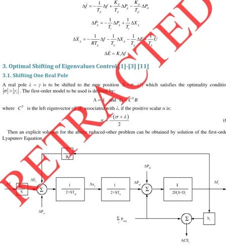
genera-tion unit supply sufficient and reliable electric power with good quality. Figure 1 shows the block diagram of

single area load frequency control. The model considered here can be written in state equations form as follows

1 p p

g d

p p p

K K

f f P P

T T T

∆ = − ∆ + ∆ − ∆

1 1

g g g

t t

P P X

T T

∆ = − ∆ + ∆

1 1 1 1

g g

g g g g

X f X E U

RT T T T

∆ = − ∆ − ∆ − ∆ +

i

E K f

∆ = ∆

3. Optimal Shifting of Eigenvalues Control [1]-[3] [11]

3.1. Shifting One Real Pole

A real pole λ = γ is to be shifted to the new position S=σ [3] which satisfies the optimality condition

i

σ >γ . The first-order model to be used is defined by:

λ

Λ = and G=C BT

where T

C is the left eigenvector of 𝐴𝐴 associated with λ, if the positive scalar α is:

(

)

2

σ λ

− +

∝ = (6)

[image:5.595.82.533.212.705.2]

Then an explicit solution for the above reduced-other problem can be obtained by solution of the first-order Lyapunov Equation

Figure 1. Block diagram of single area load frequency control.

(6)

(

σ+ ∝

)

V +V

(

σ+ ∝ =

)

H (7)

Is given by

(

)

2

H V

σ

=

+ ∝



 where:

1 T

H =GR G− (8)

Then the required parameters P Q K, ,  can be calculated as K =R G PQ−1 T = ∝2 P and P =V−1 then, the parameter rewritten as:

(

)

4

(

)

2

(

)

1 T

2 , and

P Q K R G

H H H

σ+ ∝ ∝ σ+ ∝  σ+ ∝  −

= = _{= } _

 



 

   (9)

3.2. Shifting a Complex Pole

A complex conjugate pair of poles λ, λ γ= ± jβ of Equation (3) is to be shifted to the new positions S;

S = ±σ jβ, which satisfy the optimality condition: σ >γi .

Let positive scalar α as:

(

)

2

σ λ

− +

∝ = .

The second-order model Λ to be used is define

T

T T 1

T 2

, G C B and C C

C

γ β

β γ

 

−

 

Λ =_ _ = _{=  }

−

    (10)

where

(

C1T+ jC2T

)

is the left eigenvector of A associated with the pole λ λ= + jβ and the left eigenvector

satisfied the equation:

T _Λ T

C A= C (11)

By solving the following second-order linear Lyapunov Equation of Equation (7)

(

)

(

T

)

1 T

I V V I H

H GR G−

Λ+ ∝ + Λ + ∝ =

=

  

 (12)

The parameters P Q K, ,  of the second-order optimal problem are obtained

1 T 1

, 2 and

K =R G P Q−   = ∝P P=V− (13)

Therefore, the feedback controller Kfb can be calculated from:

T fb

K =KC (14)

where

T

P=CPC (15)

2

Q= ∝P (16)

3.3. Shifting Several Poles

Problem of shifting several poles may be solved by the recursive applications of the following reduced order op-timal shifting problem

Λ

i i i i i

Z = Z +G U (17)

i i

U =K Z (18)

(

T T

)

0 d

i i i i i i

J =

∫

∞ Z Q Z +U RU t (19)

with

(7)

49

T Λ T T

,

i i i i i i

C A = C G =C B (20)

and

1

i i i

A+ =A −BK

T

and

i i i i

k =K C A = A (21)

From Equation (18), the feedback matrix K can be constructed by the summation of the optimal feedback

ma-trix Ki. Also the resulting matrices Q and P can be constructed as shown by the summation of the matrices Qi

and Pi, respectively [1]

, and

i i fb i

i i i

P=

∑

P Q=

∑

Q K =

∑

K (22)

where:

T T

, and 2

i i i i i i i i i i

k =K C P=C PC Q = ∝ P

4. Pole Placement Control [6]-[8]

By using full-state feedback can shift the poles to the left hand side by (10% - 15%). We could use the Matlab

function place to find the control vector gain K, which will give the desired poles.

(

)

place , ,

K= A B P (23)

where:

A: system matrix

B: input vector

P: pole shifting vector

K: control gain

A state feedback matrix K such that the eigenvalues of A− ∗B K are those specified in vector P. The

feed-back law of u= −kx has closed loop poles at the values specified in vector P.

(

)

Poles=eig A B K− ∗

5. Digital Simulation Results

The normal parameters of single area power system are:

0.2 sec, 0.5 sec, 1.25, 12.5 sec, 1 20, 2, 15 sec.

g t A A p p

T = T = K = T = R= K = T =

The A and B matrices of single area model are calculated as:

0.06 0.13 0 0

0 2.0 2.0 0

100 0 5 5

0.6 0 0 0

A

−

 

 ₋ 

 

=

− − − 

 

 

The dominant poles can be rewrite as:

0.4752 j2.1053

− ±

2

1

n j n

ξω ω ξ

− ± − (24)

where;

ξ: damping coefficient

n

ω : Frequency

0.478

n ξω = −

2

1 2.053

n

jω −ξ = j

(8)

0.22

ξ =

2.1

n ω =

The settling time Ts =72.7 sec. the desired value of the damping coefficient can be choosing as ζ = 0.82 to

damping the oscillation of speed and constant imaginary part. The closed loop poles are specified as:

0.82

ζ = and jω_n 1−ξ2 = j2.05

From Equation (24), calculate the ω =n 3.568 the new dominant eigenvalues can be calculated as follows

2

1 2.92 2.053

n j n j

ξω ω ξ

− ± − = − ±

The complete new poles are become as:

1,2 2.92 2.053

S = ±σ jβ = − ± j

3 6.08 S = −

4 0.0298

S = −

and calculate the settling time decreased (Ts) from 72.7 to 1 sec.

Shifting complex poles λ1,2 to S1,2, it can get:

(

)

1

0.4752 2.92

1.7040 2

− −

∝ = − =

T 1

C : left eigenvector which satisfy the Equation (10)

T 1

7.27 0.23 0.195 0.35

11.07 0.64 0.198 0.55

C = − − _

− − − −

 

Form Equation (10) Λ 0.478 2.05

2.05 0.478

−

 

= ₋ ₋ 

 

From Equations (11-12)

1

0.9706

1.4767

G =  _

 

1

0.94 1.433

1.433 2.18

H =  _

 



Therefore, the solution of the corresponding second order Lyapunov Equation is found. From Equation (12)

0.313 0.042

0.042 0.960

V =  _

 



From Equation (13)

1 1

3.213 0.142

0.142 1.04

P=V− =  − _

−

 

 

[

]

1 T

1 1 1 2.908 1.409

K =R G P−  =

1 1 1

10.95 0.484 2

0.484 3.569

Q = ∝ P =  − _

−

 

 

From Equations (14)-(16), the feedback controller gain matrix can be calculated as:

[

]

T

1 1 36.78 0.222 0.222 1.813

K =KC = − − −

(9)

51

T 1 1 1 1

275.8500 1.6665 2.1656 13.6008

1.6665 1.6665 0.0013 0.0002

2.1656 0.3090 0.1749 0.1002

13.6008 0.0955 0.1002 0.6709

P C PC

−

 

 ₋ 

 

= =

− − 

 

−

 



1 1 1

940.09 5.6795 7.3805 46.3517

5.6795 2.2740 1.0531 0.3256 2

7.3805 1.0531 0.5959 0.3416

46.3517 0.3256 0.3416 2.2863

Q P

−

 

 

= ∝ =

− − 

 ₋ 

 

Also, another shifting real pole from −0.0296 to −15 Calculate K2, P2 and Q2 as last.

[

]

2 1000 0.1123 0.0059 0.0032 1.4659

K = ∗ − − − −

From Equation (23) the K total, P total and Q total are calculated as follows:

1 2

K =K +K , P= +P1 P2, Q=Q1+Q2 as follows:

0.0112 0.0005 0.0002 0.1101

0.0005 0.0000 0.0000 0.0058 1.0e 05

0.0002 0.0000 0.0000 0.0032

0.1101 0.0058 0.0032 1.4354

P

 

 

= + ∗

 

 

0.0136 0.0007 0.0004 0.1653

0.0007 0.0000 0.0000 0.0087 1.0e 06

0.0004 0.0000 0.0000 0.0048

0.1653 0.0087 0.0048 2.1573

W

 

 

= + ∗

 

 

The total control signal K is:

[

]

optimal pole-shifting 1000 0.1491 0.0061 0.0030 1.4677

K = ∗ − − − −

And also, the feedback control from the Pole Placement Control Design is the follows:

From Equation (23), desired vector P as: P= −

[

7.0811, 0.6780− +2.0534 , 0.6780 2.0534 , 2.296i − − i −

]

. The gain matrix K=place

(

A B, ,P

)

[

]

pole placement 27.4982 1.1708 0.7619 95.9647

K = − − − −

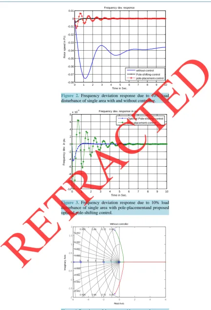
Figure 2 shows the frequency deviation response due to 10% load disturbance of single area with and without controller. The frequency is more damping in case of optimal pole shifting controller than other controller in all

disturbance and any change in operating points. Figure 3 depicts the frequency deviation response due to 10%

load disturbance of single area with pole-placement and proposed optimal pole-shifting control. Figure 4

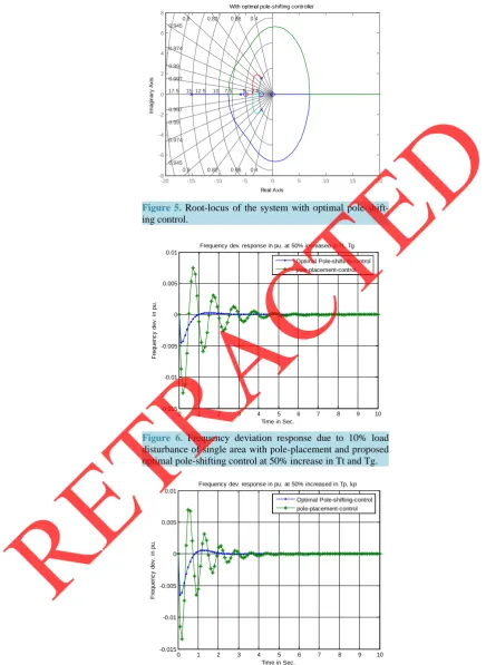
dis-plays the root-locus of the system without control. Figure 5 shows the root-locus of the system with optimal

pole-shifting control. Figure 6 depicts the frequency deviation response due to 10% load disturbance of single

area with pole-placement and proposed optimal pole-shifting control at 50% increase in Tt and Tg. Also, Figure

7 shows the frequency deviation response due to 10% load disturbance of single area with pole-placement and

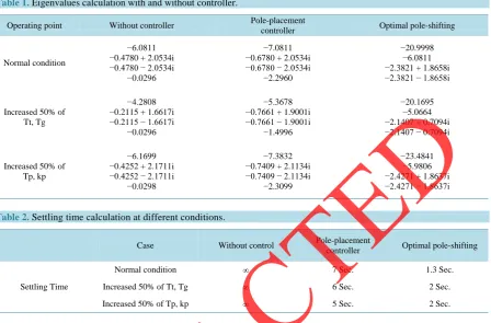
proposed optimal pole-shifting control at 50% increase in Tp and Kp. Table 1 displays the eigenvalues

calcula-tion with and without controller. Table 2 depicts the settling time calculation at different load conditions.

From Table 1, the eigenvalues of the system in case of optimal pole-shifting controller is more damping than

pole-placement control.

6. Conclusions

The present paper introduces a new controller for damping quickly the power system frequency. The problem of shifting the real parts of the open-loop poles to desired locations, while preserving the imaginary parts has been contributed. Load-frequency control (LFC) of single area systems is evaluated with two control strategies.

(10)

Figure 2. Frequency deviation response due to 10% load

disturbance of single area with and without controller.

Figure 3. Frequency deviation response due to 10% load disturbance of single area with pole-placementand proposed

[image:10.595.76.510.74.711.2]

optimal pole-shifting control.

Figure 4. Root-locus of the system without control.

0 1 2 3 4 5 6 7 8 9 10

-0.08 -0.07 -0.06 -0.05 -0.04 -0.03 -0.02 -0.01 0 0.01

Time in Sec.

R

ot

or

s

peed i

n P

U

.

Frequency dev. response

without-control Pole-shifting-control pole-placement-control

0 1 2 3 4 5 6 7 8 9 10

-12 -10 -8 -6 -4 -2 0 2 4 6 8x 10

-3

Time in Sec.

F

requenc

y

dev

. i

n pu.

Frequency dev. response in pu.

Optimal Pole-shifting-control pole-placement-control

-6 -4 -2 0 2 4 6

-2 -1.5 -1 -0.5 0 0.5 1 1.5 2

0.45 0.72 0.86 0.925 0.962

0.982

0.992

0.998

0.45 0.72 0.86 0.925 0.962 0.982 0.992 0.998

1 2 3 4 5

Without controller

Real Axis

Im

agi

nar

y

A

x

is

(11)

53

Figure 5. Root-locus of the system with optimal pole-shift-

ing control.

Figure 6. Frequency deviation response due to 10% load disturbance of single area with pole-placement and proposed

optimal pole-shifting control at 50% increase in Tt and Tg.

Figure 7. Frequency deviation response due to 10% load disturbance of single area with pole-placement and proposed

optimal pole-shifting control at 50% increase in Tp and Kp.

-20 -15 -10 -5 0 5 10 15 20

-8 -6 -4 -2 0 2 4 6 8

0.4 0.66 0.82 0.9 0.945

0.974

0.99

0.997

0.4 0.66 0.82 0.9 0.945 0.974 0.99 0.997

2.5 5 7.5 10 12.5 15 17.5 0

With optimal pole-shifting controller

Real Axis

Im

agi

nar

y

A

x

is

0 1 2 3 4 5 6 7 8 9 10

-0.015 -0.01 -0.005 0 0.005 0.01

Time in Sec.

F

requenc

y

dev

. i

n pu.

Frequency dev. response in pu. at 50% increased in Tt, Tg

0 1 2 3 4 5 6 7 8 9 10

-0.015 -0.01 -0.005 0 0.005 0.01

Time in Sec.

F

requenc

y

dev

. i

n pu.

Frequency dev. response in pu. at 50% increased in Tp, kp

[image:11.595.74.511.85.683.2]

(12)

[image:12.595.91.540.88.383.2]

Table 1. Eigenvalues calculation with and without controller.

Operating point Without controller Pole-placement

controller Optimal pole-shifting

Normal condition

−6.0811 −0.4780 + 2.0534i −0.4780 − 2.0534i

−0.0296

−7.0811 −0.6780 + 2.0534i −0.6780 − 2.0534i

−2.2960

−20.9998 −6.0811 −2.3821 + 1.8658i −2.3821 − 1.8658i

Increased 50% of Tt, Tg

−4.2808 −0.2115 + 1.6617i −0.2115 − 1.6617i

−0.0296

−5.3678 −0.7661 + 1.9001i −0.7661 − 1.9001i

−1.4996

−20.1695 −5.0664 −2.1407 + 0.7094i −2.1407 − 0.7094i

Increased 50% of Tp, kp

−6.1699 −0.4252 + 2.1711i −0.4252 − 2.1711i

−0.0298

−7.3832 −0.7409 + 2.1134i −0.7409 − 2.1134i

−2.3099

−23.4841 −5.9806 −2.4271 + 1.8637i −2.4271 − 1.8637i

Table 2. Settling time calculation at different conditions.

Case Without control Pole-placement

controller Optimal pole-shifting

Settling Time

Normal condition ∞ 7 Sec. 1.3 Sec.

Increased 50% of Tt, Tg ∞ 6 Sec. 2 Sec.

Increased 50% of Tp, kp ∞ 5 Sec. 2 Sec.

It has been shown that the shift can be achieved by an optimal feedback control law with respect to a quadratic performance index. However, this has been done without any solving non-linear algebraic Riccati Equation. Moreover, the power system is subjected to different disturbances, and also, a comparison between the power system responses using the conventional pole-placement controller and the proposed optimal pole-shifting con-troller is presented and obtained.

The digital simulation result shows the powerful of the proposed optimal pole shifting controller than conven-tional pole-placement controller in sense of fast damping oscillation and small settling time. Moreover, the op-timal pole shifting controller has less overshoot and under shoot than pole-placement control.

7. Discussions

Figures 2-7 show the frequency deviation response due to 10% load disturbance of single area with and without controller. All the response frequency is more damping in case of proposed optimal pole shifting controller than

other pole-placement controller in all disturbance and any change in operating points. From Table 1, the

eigen-values are more shifting to left hand side in case of proposed optimal pole-shifting controller than pole-place-

ment controller. Also, as shown in Table 2 the settling time is less with optimal pole-shifting controller than

other controller.

References

[1] El-Sherbiny, M.K., Hasan, M.M., El-Saady, G. and Yousef, A.M. (2003) Optimal Pole Shifting for Power System Sta-bilization. Electric Power System Research Journal, 66, 253-258.

[2] Amin, M.H. (1985) Optimal Pole Shifting for Continuous Multivariable Linear Systems. International Journal of Con-trol, 41, 701-707.

[3] Kishor, N., Saini, R.P. and Singh, S.P. (2005) Optimal Pole Shift Control in Application to a Hydro Power Plant.

Journal of Electrical Engineering, 56, 290-297.

[4] El-Sherbiny, M.K., El-Saadyand, G. and Yousef, A.M. (2002) Efficient Fuzzy Logic Load-Frequency Controller.

Energy Conversion & Management Journal, 43, 1853-1863.

[5] El-Saady, G., El-Sadek, M.Z. and Abo-El-Saud, M. (1997) Fuzzy Adaptive Model Reference Approach-Based Power

(13)

55

System Static VAR Stabilizer. Electric Power System Research, 45, 1-11.

[6] Medanic, J., Tharp, H. and Perkins, W. (1988) Pole Placement by Performance Criterion Modification. IEEE Transac-tions on Automatic Control, 33, 469-472.

[7] Rousan, N. and Sawan, M. (1991) Pole Placement by Linear Quadratic Modification for Discrete Time Systems. In-ternational Journal of Systems Science, 26-28 June 1991, 122-123.

[8] Tharp, H.S. and Perkins, W.R. (1989) Pole Placement by Performance Criterion Modification. IEEE Transactions on Automatic Control, 33, 469-472.

[9] Kishor, N., Singh, S.P. and Raghuvanshi, A.S. (2006) Dynamic Simulation of Hydro Turbine and Its State Estimation Based LQ Control. Energy Conversion and Management, 47, 3119-3137.

[10] Herron, J. and Wozniak, L. (1991) A State-Space Pressure and Speed-Sensing Governor for Hydro Generators. IEEE Transactions on Energy Conversion, 6, 414 -418.

[11] Yousef, A.M. and Kassem, A.M. (2011) Optimal Pole Shifting Controller for Interconnected Power System. Energy Conversion and Management Journal, 52, 2227-2234.