Pair copula constructions to determine the dependence structure of Treasury bond yields

REVIEW ARTICLE

Pair copula constructions to determine the

dependence structure of Treasury bond yields

Marcelo Brutti Righi, Sergio Guilherme Schlender

*,

Paulo Sergio Ceretta

Federal University of Santa Maria, Department of Business, University of Santa Maria, Santa Maria, Rio Grande do Sul 97105-900, Brazil

Received 24 September 2013; revised 22 January 2015; accepted 7 October 2015; available online 23 October 2015

KEYWORDS Treasury bonds; Pair copula construction;

Dependence structure

Abstract We estimated the dependence structure of US Treasury bonds through a pair copula construction. As a result, we verified that the variability of the yields decreases with a longer time of maturity of the bond. The yields presented strong dependence with past values, strongly positive bivariate associations between the daily variations, and prevalence of the Student’s t copula in the relationships between the bonds. Furthermore, in tail associations, we identified relevant values in most of the relationships, which highlights the importance of risk manage-ment in the context of bonds diversification.

© 2015 Production and hosting by Elsevier Ltd on behalf of Indian Institute of Management Bangalore.

Introduction

Since the introduction of the mathematical theory of portfolio selection and of the capital asset pricing model (CAPM), the issue of dependence has always been of fundamental importance to financial economics. In the context of international diversifi-cation, there is a need to minimise the risk of specific assets (such as stocks and Treasury bonds) through optimal allocation of resources. Many studies have used a statistical model which is able to measure the temporal dependence between stocks

and Treasury bonds:Campbell and Ammer (1993)apply a vector autoregressive (VAR) system in AMEX and NYSE stocks and US Treasury bonds, but they do not analyse the effect of the vola-tility of the relationship.Li (2002)andKim, Moshirian, and Wu (2006)estimate a bivariate generalised autoregressive condi-tional heteroscedasticity (GARCH) model and bivariate expo-nential GARCH with t-distribution and verify important implications in stock-bonds correlation. However,Cappiello, Engle, and Sheppard (2006), andLi and Zou (2008)expand the asymmetric and multivariate approach with dynamic condi-tional correlation (DCC) GARCH.

Traditionally, correlation is used to describe the depen-dence between random variables, but recent studies, such as that conducted byEmbrechts, Lindskog, and McNeil (2003), have ascertained the superiority of copulas to model depen-dence. Copulas offer much more flexibility than the correlation

* Corresponding author. Tel.:+55 55 9659 5220; fax:+55 55 3220 9258.

E-mail address:[email protected](S.G. Schlender). Peer-review under responsibility of Indian Institute of Management Bangalore.

IIMB Management Review (2015)27, 216–227

a v a i l a b l e a t w w w. s c i e n c e d i r e c t . c o m

ScienceDirect

j o u r n a l h o m e p a g e : w w w. e l s e v i e r. c o m / l o c a t e / i i m b

http://dx.doi.org/10.1016/j.iimb.2015.10.008

0970-3896 © 2015 Production and hosting by Elsevier Ltd on behalf of Indian Institute of Management Bangalore.

approach because a copula function can deal with non-linearity, asymmetry, serial dependence and also the well-known heavy-tails of financial assets’ marginal and joint probability distribution. In studies of Treasury bonds,Junker, Szimayer, and Wagner (2006)apply the normal copula model in US Treasury monthly bonds, confirming the importance of this approach in considering tail dependence and symme-try.Lee, Kim, and Kim (2011)apply Archimedean copulas in interdependence of US, UK, and Japan interest rates, ac-cording to different maturities of bonds. This paper verifies that both negative and positive returns in the US and UK move in a similar trend whereas in Japan interest rates follow a dif-ferent trend.Diks et al. (2014)test the forecast accuracy of copula families in 10-years maturity of G7 countries’ gov-ernment bonds, where the Student’s t and Clayton mixture copula outperforms the other copulas considered.

A copula is a function that links univariate marginals to their multivariate distribution. Since it is always possible to map any vector of random variables into a vector with uniform margins, we are able to split the margins of that vector, which is the copula. Although the literature on copulas is consis-tent, the great part of the research is still limited to the bi-variate case. Thus, constructing higher dimensional copulas is the natural next step, but this is not an easy task. Apart from the multivariate Gaussian and Student (see work in stock-bonds structure dependence ofKang, 2007), the selection of higher-dimensional parametric copulas is still rather limited (Genest, Rémillard, & Beaudoin, 2009).

The developments in this area tend to hierarchical, copula-based structures. It is possible that the most promising of these is the pair copula construction (PCC). Originally proposed by Joe (1996), it has been further discussed and explored in the literature for questions of inference and simulation. The PCC is based on a decomposition of a multivariate density into bi-variate copula densities, of which some are dependency struc-tures of unconditional bivariate distributions, and the rest are dependency structures of conditional bivariate distribu-tions. Applications to financial data have shown that these vine-PCC models outperform other multivariate copula models in predicting log-returns of equity portfolios.Min and Czado (2010)present a PCC copula model in daily returns from January 1, 1999 to July 8, 2003 of the Norwegian stock index, the MSCI world stock index, the Norwegian bond index and the SSBWG hedged bond index, and they verify a stronger de-pendence between international bonds and stocks, interna-tional and Norwegian stocks, and Norwegian stocks and bonds, but they observe that the Norwegian bond index does not depend on the MSCI world stock index if the Norwegian stock index is given. In this context, this paper poses the ques-tion: What would the dependence structure of Treasury bonds be in relation to their maturity?

To answer this question, this paper aims to estimate the dependence structure between Treasury bonds through a PCC. To that effect, we collected daily data from Treasury bonds of the US government for 1-, 2-, 3-, 5-, 7- and 10-years of ma-turity, which were the most sought after by investors in order to obtain truly risk free assets. The estimated structure allows the calculation of the non-linear absolute and tail depen-dences of each bivariate relationship between the bonds, iso-lating the effect of the other. It is also possible to verify which bond has more dependence with all the others, and to iden-tify the “leading” Treasury bonds.

The paper is structured as follows: The second section briefly presents the background of copulas and PCC; the third section presents the material and methods of the study, de-scribing the data and the procedures used to achieve the ob-jective of the paper; the fourth section presents the results obtained and the discussion; and the fifth section contains the conclusions of the paper; the appendix introduces the copula families utilised in this study.

Background

This section is subdivided into: i) Copula methods, which briefly defines this class of functions and describes its prop-erties; this sub section also contains a literature review; ii) Pair copula construction, which succinctly describes the concepts of this structure.

Copula methods

Dependence between random variables can be modelled by copulas. A copula returns the joint probability of events as a function of the marginal probabilities of each event. This makes copulas attractive, as the univariate marginal behaviour of random variables can be modelled separately from their dependence (Kojadinovic & Yan, 2010).

The concept of copula was introduced bySklar (1959). However, it was only recently that its applications became clear. A detailed treatment of copulas as well as of their re-lationship to concepts of dependence is given byJoe (1997) andNelsen (2006). A review of the applications of copulas to finance can be found inEmbrechts et al. (2003) and in Cherubini, Luciano, and Vecchiato (2004).

To facilitate our understanding of the concept we re-strict our attention to the bivariate case. The extensions to then-dimensional case are straightforward. A function

C:

[ ]

0 1, 2→

[ ]

0 1, is a copula if, for 0≤x≤1 and

x1 x2 y1 y2 x y1 1 x2 y2

2 0 1

≤ , ≤ ,

(

,

) (

, ,

)

∈

[ ]

, , it fulfills the follow-ing properties:

C x

( )

,1 =C

( )

1,x =x, C x

(

,0

)

=C

(

0,x

)

=0. (1)

C x

(

2,y2

)

−C x

(

2,y1

)

−C x y

(

1, 2

)

+C x y

(

1, 1

)

≥0. (2) Property (1) means uniformity of the margins, while (2), the n-increasing property means that

P x

(

1≤ ≤X x2,y1≤ ≤Y y2

)

≥0 for (X, Y) with distribution functionC.

In Sklar’s seminal paper (1959), it was demonstrated that a copula is linked with a distribution function and its mar-ginal distributions. This important theorem states:

(i) LetCbe a copula andF1andF2univariate distribution func-tions. Then (3) defines a distribution functionF with marginalsF1andF2.

F x y

(

,

)

=C F x

(

1

( ) ( )

,F y2

) (

, x y,

)

∈R2. (3) (ii) For a two-dimensional distribution functionFwith mar-ginalF1andF2, there is a copulaCsatisfying (3). This is unique ifF1andF2are continuous and then, for every

u v, ,

(

)

∈

[ ]

0 12: C u v

(

,

)

=F F

(

1−

( )

u,F−

( )

v

)

. 1 2 1 (4) In (4), F1 F 1 2 1

− _and − _{denote the generalised left}

continu-ous inverses ofF1andF2. Regarding the estimation, the domi-nant methods are the traditional maximum likelihood (ML), the pseudo-maximum likelihood (PML), proposed byGenest, Ghoudi, and Rivest (1995), and the inversion of dependence measures such as Spearman’s rho and Kendall’s tau.Chen and Fan (2006b)developed an extension of the pseudo-maximum likelihood of Markovian time series.

However, asFrees and Valdez (1998)note, it is not always possible to identify the copula. According toBerrada, Dupuis, Jacquier, Papageorgiou, and Rémillard (2006), for many fi-nancial applications, the problem is not in using a given mul-tivariate distribution but in finding a convenient distribution to describe some stylised facts, for example the relation-ships between different asset returns.Genest et al. (2009) present an overview of the goodness of fit and selection issues of copula families.

Since copulas are linked to the dependence structure, they must be related to dependence measures. We present here the calculation procedures, adapted fromCherubini, Gobbi, Mulinacci, and Romagnoli (2012), of the most representa-tive dependence measures for financial purposes. Given the estimated bivariate copulaC, the lower and upper tail de-pendence are represented by formulations(5) and (6), re-spectively. The absolute dependence calculated with Kendall’s tau through the conversion of the bivariate copula is exposed in formulation(7). λL u C u u u =

(

)

→+ lim , 0 (5) λU u u C u u u = − +

(

)

− →− lim , 1 1 2 1 (6) τ

(

x y,

)

=4

∫

∫

C u v dC u v

(

,

) (

,

)

−1. 0 1 0 1 (7) Regarding the literature on copula methods, it is note-worthy that there was a significant growth in the number of applications of this technique in the last few years. With ref-erence to time series, one of the most appealing approaches is the time-varying copulas, which consist of the change of the shape and parameters of the estimated copula families along time. Some of the most structured proposals on the topic are the works ofChen and Fan (2006a, 2006b)andPatton (2006, 2011). As a financial application of dynamic copulas, we can cite the work ofGoorbergh, Genest, and Werker (2005) in option pricing.

Further, the estimation of serial dependence with copulas has emerged as an important approach to financial studies. This approach was first proposed byDarsow, Nguyen, and Olsen (1992) and extended in the recent works ofAbegaz and Naik-Nimbalkar (2008), Ibragimov (2009), Chen, Wu, and Yi (2009)andBeare (2010). The extension of these researches with the inclusion of cross-interdependence in Markovian time series is seen in the work ofRémillard, Papageorgiou, and Soustra (2011). These authors determined the dependence between the returns of the Canadian/US exchange rate and oil prices. With Treasury bonds,

Junker et al. (2006)apply copula functions in the analysis of cross-sectional nonlinear term structure dependence for US Trea-sury monthly bonds covering the period October 1982 to De-cember 2001.Kang (2007)presents a multidimensional approach with a copula-GARCH model to measure the dependence struc-ture of daily excess returns on two stock indices and two Trea-sury bonds—S&P 500 index, NASDAQ index, 1-year TreaTrea-sury bond and 10-year Treasury bond, from October 11, 1984 to October 28, 2005.Garcia and Tsafack (2011)present the dependence structure pairwise of weekly equity and 5-year bond returns of markets in the United States, Canada, France, and Germany from January 1, 1985 to December 21, 2004 with mixture copulas.

Pair copula construction

The PCC is a very flexible construction, which allows the free specification ofn(n−1)/2bivariate copulas. This construc-tion was proposed in the seminal paper byJoe (1996), and it has been discussed in detail, especially for applications in simulation and inference (Bedford & Cooke, 2001, 2002; Kurowicka & Cooke, 2006). The PCC is hierarchical by nature. The modelling scheme is based on the decomposition of a mul-tivariate density inton(n−1)/2bivariate copula densities, of which the firstn−1 are dependency structures of uncon-ditional bivariate distributions, and the rest are depen-dency structures of conditional bivariate distributions (Aas & Berg, 2011).

The PCC is usually represented in terms of density. The two main types of PCC that have been proposed in the lit-erature are the C (canonical)-vines and D-vines. In the present paper we focus on the D-vine estimation, which according to Aas, Czado, Frigessi, and Bakken (2009)has the density as in formulation(8). f x x f x c F x x x F x x x n _k k n i i i j i j i i j 1 ₁ 1 1 1 , , , , , , ,

(

)

= ₌

( )

(

+ + −

)

+ + + −

∏

1 ₁₁ 1

(

)

⎧ ⎨ ⎩ ⎫ ⎬ ⎭ = − = −

∏

∏

i i n j j n . (8) In (8),x1,…,xnare variables; fis the density function;

c

( )

⋅ ⋅, is a bivariate copula density and the conditional dis-tribution functions are computed, according toJoe (1996), by formulation(9). F x C F x F v F v x v j j j j j j j v v v v v

( )

=∂

{

(

) (

)

}

∂

(

)

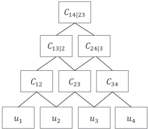
− − − − , , (9) In (9), Cx v,jv−j is the dependency structure of the bivari-ate conditional distribution ofxandvjconditioned on v−j, where the vector v₋jis the vector vexcluding the compo-nentvj. In order to make it possible to use the D-vine con-struction to represent a dependency structure through copulas, we must assume that the univariate margins are uniform in the interval [0, 1]. As an illustration, we present in formu-lation(10)a four-dimensional case, and its graphical repre-sentation inFig. 1. C u u u u C u u C u u C u u C F u u 1 2 3 4 12 1 2 23 2 3 34 3 4 13 2 1 2 , , , , , ,

(

)

=

(

)

⋅

(

)

⋅

(

)

⋅

(

(

)) (

)

)

⋅

(

(

) (

)

)

⋅

(

)

, , , , , F u u C F u u F u u C F u u u F u u u 3 2 24 3 2 3 4 3 14 23

(

1 2 3

(

4 2 33

)

)

(10) M.B. Righi et al. 218

Where F u u

(

1 2

)

= ∂C12

(

u u1, 2

)

∂u2, F u u

(

3 2

)

= ∂C23

(

u u2, 3

)

∂u2, F u u

(

2 3

)

= ∂C23

(

u u2, 3

)

∂u3, F u u

(

4 3

)

= ∂C34

(

u u3, 4

)

∂u3, F u u u

(

1 2, 3

)

= ∂C13 2

(

F u u

(

1 2

) (

,F u u3 2

)

)

∂F u u

(

3 2

)

, F u u u

(

4 2, 3

)

= ∂C24 3

(

F u u

(

4 3

) (

,F u u2 3

)

)

∂F u u

(

2 3

)

. Thus, the conditional distributions involved at one level of the construction are always computed as partial deriva-tives of the bivariate copulas at the previous level (Aas & Berg, 2011). Since only bivariate copulas are involved, the partial derivatives may be obtained relatively easily for most para-metric copula families. It is noteworthy that the copulas in-volved in (8) do not have to belong to the same family. Hence, we should choose, for each pair of variables, the paramet-ric copula that best fits the data.

With regard to the estimation of the PCC parameters,Aas et al. (2009)propose a maximum likelihood estimation pro-cedure which follows a stepwise approach. In the first step, one computes ML estimates of the parameters of each pair-copula family separately. The estimated parameters ob-tained in this first step are known as sequential ML estimates. In a second step, the full log-likelihood function is maximised jointly using the sequential ML estimates as starting values, resulting in the so-called joint ML estimates.

Regarding the literature of PCC in finance,Aas and Berg (2011)compared the nested Archimedean construction (NAC) and the PCC. They found that the NAC is much more restric-tive than the PCC in two aspects. There are strong limita-tions on the degree of dependence in each level of the NAC, and all the bivariate copulas in this construction have to be Archimedean. Further, they show that the PCC provides a better fit than the NAC and that it is computationally more efficient.

Chollete, Heinen, and Valdesogo (2009)construct a multi-variate regime-switching model of copulas for returns from the G5 and Latin American regions. They document that models with canonical vines generally dominate alternative depen-dence structures; they also document the importance of the models for risk management, since they modify the Value-at-Risk (VaR) of international portfolios and produce a better out-of-sample performance.Fischer, Köck, Schlüter, and Weigert (2009)empirically investigate whether PCC models are really capable of outperforming the Student’s t copula. In addition, the authors compare the fit of PCC models among other copula estimators.Min and Czado (2010)develop a Markov chain Monte Carlo (MCMC) algorithm which allows interval es-timation by means of credible intervals for Kendall’s and tail dependence coefficient of daily returns of Norwegian stock index, MSCI world stock index, Norwegian bond index and SSBWG hedged bond index from January 1, 1999 to July 8, 2003. This algorithm reveals unconditional as well as condi-tional independence in the data which can simplify resulting PCCs.Czado, Schepsmeier, and Min (2012)verify the fit of multivariate dependence models, including PCC, in the re-lationships of exchange rates. Their findings corroborate the superiority of the PCC models for this purpose.Righi and Ceretta (2012a)conducted VaR predictions of three sets of markets: developed, emerging Latin, and emerging Asian-Pacific. With the same data,Righi and Ceretta (2012b)evaluated the dif-ferences on tail dependence between the market groups.

Methodological procedures

We collected daily yields for 1-, 2-, 3-, 5-, 7- and 10-years’ maturity Treasury bonds of the US government, from January 2, 1990 to April 12, 2012, totalling 5573 observations. These bonds were chosen because the US money market is tradi-tionally considered by investors as the best source of risk free assets. The choice of this period was due to the combina-tion of the availability of data in the website of the US De-partment of Treasury and the need for collection of information over a length of time in order to avoid band-width biases. We excluded from the analysis those bonds that did not have negotiations during the whole period. Also, there is always a computational concern with the high-dimensionality of data, obligating the research to choose parsimoniously which variables to include in a model. Reinforcing the option for these bonds, it is worth mentioning that they are, in general, the most liquid.

Seeking to avoid issues relative to the non-stationary con-dition, we calculated the logarithmic differences (log-returns) of the collected daily yields. We modelled the marginal of these log-returns through autoregressive moving average (ARMA (m,n)) – generalised autoregressive condi-tional heteroscedastic (GARCH (p,q)) models with student in-novations, in order to consider the well-known conditional heteroscedastic heavy-tailed behaviour of the financial assets (Longin & Solnik, 2001). The estimated model is repre-sented in formulations(11) to (13).

ri t, =μi +

∑

φi m i t m, r,− +

∑

θ εi n i t n, ,− +εi t, (11)

εi t, =h zi t i t, ,, zi t, ∼tv (12)

hi t2, =ωi+

∑

α εi p i t p, 2,− +

∑

βi q i t q,h2,−. (13)

where ri t, is the log-return of assetiin periodt;hi t, 2

is the conditional variance of assetiin periodt;µi,ϕi,θi,ωi,αiand βiare parameters;εi t, is the innovation in the conditional mean of asseti in period t; zi t, represents the white noise of t-student distribution. The models were validated through the verification of serial correlation in the linear and squared stan-dardised residuals through theQstatistic, represented for (14).

Q n n n k k k h =

(

+

)

− =

∑

2 2 1 ˘ ρ ₍₁₄₎

In (14),nis the size of sample; ˘ρk2

is the autocorrelation of sample in lagk;his the number of lags being tested. The Qstatistics, which test the null hypothesis of randomness of data, follow a chi-squared

( )

χ2 _{distribution withhdegrees} of freedom.

After modelling the marginal, we estimated the PCC com-posed of the sector indexes. We standardised the residuals of the GARCH approach into pseudo-observations

Uj =

(

U1j,…,Uij

)

through the ranks as Uij =Rij

(

n+1

)

. We ordered the variables by decreasing order of the sum of the non-linear dependence, measured through Kendall’s tau, with the other variables. Subsequently, to choose the copula that best fit each bivariate pair of variables we employed the AIC criterion. A more detailed presentation of the copula fami-lies present in this selection is given in the appendix. The es-timation of the parameters followed the procedure presented in the section on materials and methods. We converted the estimated parameters in the association measures pre-sented in the section on materials and methods.

To validate the choice of a D-vine PCC, we compared the estimated model with the counterpart C-vine by the test pro-posed byClarke (2007). For this, letC1and C2be two com-peting vine copulas in terms of their densities and with estimated parameter setsθ1andθ2. The null hypothesis of sta-tistical indifference of the two models is:

H P m m C u C u n i i i i i 0 1 1 2 2 0 0 5 1 :

(

>

)

= . , =log⎡ , , , . ⎣ ⎢

(

(

θ_θ

)

)

⎤_⎦⎥ ∀ = … (15)

Results and discussion

This section is divided, for best comprehension, into two parts: i) marginal modelling, which exposes the descriptive char-acteristics of the studied data, as well as the results of the marginal models estimation; and ii) conditional depen-dence modelling, which presents the results for the esti-mated PCC, and also its implications for the Treasury bond market.

Marginal modelling

Initially we collect data for the daily yield for the US Treasury bonds with 1-, 2-, 3-, 5-, 7- and 10-years of maturity. A study of the collected data for the daily yield for the US Treasury bonds with 1-, 2-, 3-, 5-, 7- and 10-years of maturity (totalling 5573

observations) shows that the daily yields of all maturities pre-sented a common evolution along the sample.1_{This long term}

equilibrium is expected, since the bonds are linked by a mutual monetary policy which is managed through variables as the basic interest rate and the inflation. It is valid to emphasise that the expected yield rises with the maturity of its respective bond, as reflected by the well-known yield curves.

Another fact that emerges is the fall in the yield rates during periods of economic turbulence, as the 1993/1994 stag-nation (observations 800–1200), the crisis in emerging markets in the decade of the 90s (observations 1500-2300), the ter-rorist attacks in 2001 (observations 3000-3500), the sub-prime and Euro-zone crisis (observations 4500 to the present). These falls in the yield are intrinsically linked with the attempt of the US government to promote the economy through an expansionist monetary policy with low interest rates, ac-cording toMiao, Wu, and Su (2013). It follows that this situ-ation is very strong and continual in financial crises volatility and linked to the expectation of falling interest rates, where investors would prefer Treasury bond rather than short-term bond.

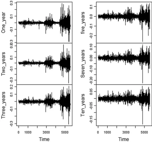
In order to avoid the non-stationary behaviour of the yield curves in level,2_{we calculated their log-returns. The plots}

with the time series of the log-returns of the analysed Trea-sury bonds during the sample period are presented inFig. 2. The plots inFig. 2reveal, again, the presence of a similar temporal evolution in the series. There were notorious vola-tility clusters during the turbulent periods previously men-tioned, which coincide with the falls in the yields. This result corroborates the stylised fact of financial assets which attests that there is more volatility in falls than in rises. Moreover, the dispersion around the long term mean appears to be larger for the bonds with more maturity time during the calm periods, and for those with less maturity time during the periods of strong economic turbulence.

Complementing this descriptive analysis,Table 1 pres-ents some statistics for the daily log-returns of the U.S. Trea-sury bond yields. The results contained inTable 1firstly indicate that the daily yields of the Treasury bonds had an expected value very close to zero, as pointed out by the central tendency measures. Moreover, the bonds presented great range (maximum—minimum) and dispersion (standard deviation) during the analysed period. This variability de-creases with the time of maturity of the bond (same obser-vations are made byJunker et al., 2006, when analysing 1-, 2-, 3-, 4- and 5-years of maturity from 1982 to 1991 and from 1992 to 2001 subsample periods), confirming the fact that the bonds with less time of maturity were more sensitive to the economic turbulences which occurred in the sample. Further, all series are leptokurtic and negative asymmetric.3

These descriptive results confirm the well-known stylised facts about financial assets, previously cited in this paper. Thus, it is necessary to use flexible techniques in order to model both the marginal and the joint evolution of this kind

1_{We performed cointegration tests which statistically confirmed the}

long term equilibrium among all the analysed bonds.

2_{We performed unit root tests in the series of the Treasury bond yields}

which showed as non-stationary in the level but stationary in the loga-rithmic difference.

3 _{We performed tests of normality which were rejected for all the}

series of the log-returns of the Treasury bond yields.

M.B. Righi et al. 220

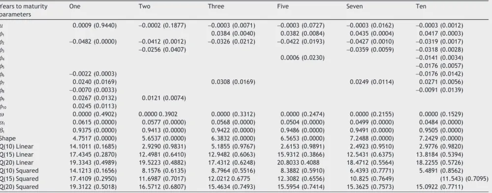
of variable. Regarding the marginal,Table 2presents the es-timated parameters, as well as the diagnostics of the ARMA-GARCH models utilised to model the studied log-returns.

The results contained inTable 2clearly indicate that the daily log-returns of the yields were very persistent during the studied period, as one can perceive by the significance4_of

the auto-regressive parameters. This influence of the lagged variations in the yields can be explained by the fact that the chosen period is very large and it contains some economic tur-bulence, which leads to a rise in the dependence on past in-formation. Further, some bonds, especially those with longer time of maturity, presented a value for their unconditional mean significantly different from zero.

Regarding the conditional variance, all the log-returns of the US Treasury bond yields were significantly affected by the squared deviations from their expected value, as well as by the conditional variance from the last day of negotiation. Moreover, the estimated ARMA-GARCH models were vali-dated through theQstatistic. The null hypothesis of no de-pendence on past information was not rejected for any of the bonds, both for the linear standardised residuals as for their quadratic form.

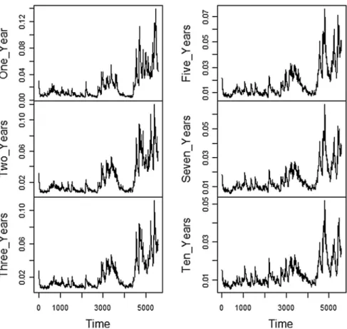
Complementing this,Fig. 3exposes the daily conditional volatilities of the log-returns of the US Treasury bond yields in the sample period obtained through the ARMA-GARCH models. The plots visually confirm the previous results that infer a presence of volatility clusters in the cited turbulent periods. Again, the peak of the dispersion occurred during the sub-prime and Euro-zone crisis. Further, the level of the

4 _{The significance level of 5% was chosen.}

Figure 2 Daily log-returns of the yield of US Treasury bonds with 1-, 2-, 3-, 5-, 7- and 10-years of maturity from January 2, 1990 to April 12, 2012, totalling 5573 observations.

Table 1 Descriptive statistics of daily log-returns of yield of U.S. Treasury bonds with 1-, 2-, 3-, 5-, 7- and 10- years of matu-rity from January 2, 1990 to April 12, 2012, totalling 5573 observations.

Years to maturity One Two Three Five Seven Ten

Minimum −0.2877 −0.3514 −0.3102 −0.2614 −0.2241 −0.1850 Maximum 0.2962 0.3185 0.2097 0.1323 0.1169 0.0892 Mean −0.0006 −0.0006 −0.0005 −0.0004 −0.0003 −0.0002 Median 0.0000 0.0000 0.0000 0.0000 0.0000 0.0000 St. deviation 0.0299 0.0310 0.0277 0.0217 0.0180 0.0149 Skewness −0.1854 −0.1208 −0.2611 −0.3307 −0.2120 −0.2702 Kurtosis 18.1012 14.0731 12.6722 11.1843 9.8191 8.4624

Table 2 Estimated parameters*and diagnostics**of the linear and squared residuals of the estimated ARMA-GARCH modelsa_{for the daily log-returns of the yield of U.S.} Trea-sury bonds with 1-, 2-, 3-, 5-, 7- and 10-years of maturity from January 2, 1990 to April 12, 2012, totalling 5573 observations.

Years to maturity parameters

One Two Three Five Seven Ten

µ 0.0009 (0.9440) −0.0002 (0.1877) −0.0003 (0.0071) −0.0003 (0.0727) −0.0003 (0.0162) −0.0003 (0.0012) ϕ1 0.0384 (0.0040) 0.0382 (0.0084) 0.0435 (0.0004) 0.0417 (0.0003) ϕ2 −0.0482 (0.0000) −0.0412 (0.0012) −0.0326 (0.0212) −0.0422 (0.0193) −0.0427 (0.0010) −0.0319 (0.0017) ϕ3 −0.0256 (0.0407) −0.0359 (0.0059) −0.0318 (0.0028) ϕ4 0.0006 (0.0230) −0.0141 (0.0034) ϕ5 −0.0176 (0.0057) ϕ6 −0.0022 (0.0003) −0.0176 (0.0142) ϕ7 0.0240 (0.0169) 0.0308 (0.0169) 0.0249 (0.0114) 0.0271 (0.0056) ϕ8 −0.0070 (0.0033) −0.0091 (0.0139) ϕ9 0.0267 (0.0132) 0.0121 (0.0074) ϕ10 0.0245 (0.0113) ω 0.0000 (0.4902) 0.0000 0.3902 0.0000 (0.3312) 0.0000 (0.2474) 0.0000 (0.2155) 0.0000 (0.1529) α1 0.0615 (0.0000) 0.0577 (0.0000) 0.0568 (0.0000) 0.0504 (0.0000) 0.0499 (0.0000) 0.0484 (0.0000) β1 0.9375 (0.0000) 0.9413 (0.0000) 0.9422 (0.0000) 0.9486 (0.0000) 0.9491 (0.0000) 0.9505 (0.0000) Shape 4.7517 (0.0000) 5.6537 (0.0000) 6.3832 (0.0000) 6.5653 (0.0000) 7.2488 (0.0000) 7.2429 (0.0000) Q(10) Linear 14.1011 (0.1685) 2.9290 (0.9831) 5.1855 (0.9767) 2.6153 (0.9891) 2.4923 (0.9510) 2.9776 (0.9820) Q(15) Linear 17.4345 (0.2870) 12.4981 (0.6410) 12.9482 (0.6063) 15.9312 (0.3866) 12.5431 (0.6375) 13.8184 (0.5394) Q(20) Linear 19.3343 (0.4989) 19.5223 (0.4882) 17.4312 (0.6248) 20.8033 0.4088 18.4712 (0.5564) 18.2255 (0.5726) Q(10) Squared 14.1213 (0.1656) 8.1576 (0.6135) 8.7964 (0.5516) 8.3882 (0.5910) 6.4393 (0.7771) 5.4891 (0.8562) Q(15) Squared 17.4109 (0.2950) 11.6987 (0.7017) 12.0212 0.6775 12.3082 (0.6556) 10.825 (0.7649) (11.543) (0.7095) Q(20) Squared 19.3122 (0.5018) 16.5712 (0.6807) 15.4634 (0.7493) 15.5954 (0.7414) 15.3625 (0.7573) 15.0922 (0.7711) *Parameters are defined in (11) and (13). Shape is the number of degrees of freedom of the student’stconditional distribution.

**Q(k) is the statistic forklags; p-values are in parenthesis.

a_{We chose to limit the number of auto-regressive parameters to 10 for computational and parsimony issues. However, there was no need for more lagged parameters, as explicated by the}

Qstatistics. M.B. Righi et al. 222

variability of the bonds with less time of maturity was higher than that of the bonds with more time of maturity.

Conditional dependence modelling

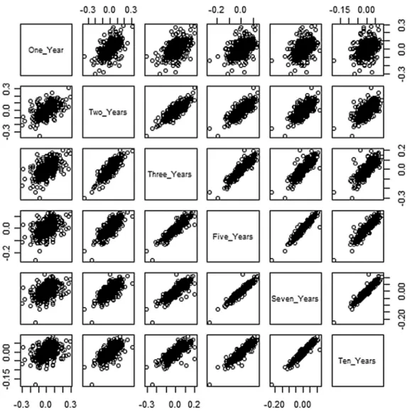
In this step we model the dependence structure of the Trea-sury bonds isolating the effect of the marginal, which were modelled through the ARMA-GARCH models. Initially, we present inFig. 4the scatter plot of the residuals of the mar-ginal models. The scatter plot ofFig. 4indicates that all the bivariate associations between the daily variations of the yields are strongly positive (Junker et al., 2006use normal copula yields and confirm this same correlation). This characteris-tic of dependence reflects, in certain degree, the long term association of the yield curve of the bonds. Moreover, the plots point out that there are associations in the extreme values (tails) of the presented relationships. This behaviour is a vestige of the need for joint distribution that considers this probability in the tails.

Subsequently, we calculated the matrix of dependence for the daily log-returns of Treasury bond yields, through the Ken-dall’s tau measure, aiming to select their order in the esti-mation of the PCC. The adopted criterion was the absolute sum of the dependence between each index with all the others. The results are presented inTable 3. The results in Table 3reinforce the presence of great dependence between the Treasury bonds. With the exception of the pair 1 year/ 10 years, all the relationships had magnitude of the non-linear

dependence over 0.5. The mean magnitude of the associa-tions was 0.69, a very large value.

Regarding the order, the bond with most dependence with the others was the 5-years, followed by 3-years, 7-years, 10-years, 2-years and 1-year of maturity. With this order we estimate, through ML, a PCC for the log-returns of the Treasury bond yields in the sample period. The results of this estimation, as well as the dependence measures asso-ciated with the parameters of the pair copulas, are presented inTable 4.

The results inTable 4initially indicate that there is an ab-solute predominance of the Student’s t copula in the bivari-ate relationships which compose the dependence structure of the US government Treasury bonds. This result corrobo-rates that of previous research, such as that performed by Marshal and Zeevi (2002)andDiks et al. (2014), which have shown that the fit of this copula family is generally superior to that of other copulas for financial data. Based on the se-lected families of the PCC estimation, it is noteworthy that these copulas assign, in certain degree, more importance to the tails of the joint probability distribution than the Gauss-ian one. This suggests that there is more dependence among the sectors in extreme events than in the normally ex-pected events.

Table 4presents the dependence measures, converted through the estimated copulas of each bivariate relation-ship. Firstly, all the measures (lower tail, upper tail, and tau) exhibited a trend for decreasing behaviour in the direction of the initial levels of the vine to the final ones, which was Figure 3 Estimated conditional volatility of the daily log-returns of yield of US Treasury bonds with 1-, 2-, 3-, 5-, 7- and 10-years of maturity from January 2, 1990 to April 12, 2012, totalling 5573 observations.

expected as this is the nature of this hierarchical construc-tion. However, some relationships in the last levels of the vines exhibited large association, as for example, the association between the bonds of 3-years and 2-years of maturity. The

separations of dependence measures in terms of maturity (at-tributed toLee et al., 2011) denote the presence of differ-ent dealing participants: active dealers tend to short-term maturities bonds and passive dealers tend to long-term maturities.

Regarding the magnitude of the dependence, the tail mea-sures obtained relevant values in most of the bivariate rela-tionships, except those in the last levels of the vine where even the absolute dependence (tau) was very low. The tail dependences were very similar to the absolute one almost in all cases. The dependences in the lower and upper tails were equal, reflecting the fact that the Student’s t copula is elliptical. It is noteworthy that the relationship between the bonds with 3-years and 10-years in the estimated PCC ob-tained negative sign, emphasising the differences that are veri-fied in the dependences between two variables when one isolates the effect of other variables.

Further, the estimated PCC rejected the null hypothesis of the Clark test, which states that there is significant dis-tinction in the fit of the utilised D-vine approach and the C-vine construction, emphasising the advantages in choosing the D-vine construction. Regarding the domain of the depen-dence, the 7-year bond presented the greatest mean for the Figure 4 Scatter plot of the estimated residuals of the ARMA-GARCH models for the daily log-returns of the yield of US Treasury bonds with 1-, 2-, 3-, 5-, 7- and 10-years of maturity from January 2, 1990 to April 12, 2012, totalling 5573 observations.

Table 3 Kendall’s tau*dependence matrix of the log-returns of the yield of the U.S. Treasury bonds with 1-, 2-, 3-, 5-, 7- and 10-years of maturity from January 2, 1990 to April 12, 2012, totalling 5573 observations.

Years One Two Three Five Seven Ten

One 1.0000 0.6392 0.5980 0.5624 0.5199 0.4912 Two 0.6392 1.0000 0.7071 0.7294 0.6654 0.6214 Three 0.5980 0.7971 1.0000 0.8149 0.7471 0.6976 Five 0.5624 0.7294 0.8149 1.0000 0.8539 0.7993 Seven 0.5199 0.6654 0.7471 0.8539 1.0000 0.8680 Ten 0.4912 0.6214 0.6976 0.7993 0.8680 1.0000 Sum 3.8107 4.4523 4.6547 4.7599 4.6543 4.4775

*The Kendall’s tau measure was chosen because it can identify non-linear dependence, unlike the traditional linear correla-tion.

M.B. Righi et al. 224

tau and tail measures, if considered in relation to the other bonds. The 5-year, which had the largest association with the others, lost dependence after the isolation of indirect effect. This can be explained by the liquidity in the negotiation of these bonds.Chordia, Sarkar, and Subrahmanyam (2005), in their in-depth study of the relationship of bonds with liquid-ity, find the association between monetary expansions and increased liquidity, in which government bond sector plays an important role in forecasting bond market liquidity.

In a general form, these results highlight the importance of risk management in terms of bonds diversification. This is because such concentration of joint probability in the tails, in particular for lower values, indicates that it can be diffi-cult to minimise the risk of a portfolio based on investment allocation in these bonds, especially in times of negative in-novations, such as a crisis, which is when active managers most need to protect their investments.Junker et al. (2006)seek to focus on this approach; however, they do not delve in depth on the relationship between Treasury bond maturities since their work is more restricted to the comparison between fami-lies of copulas.

Conclusion

This paper aimed to estimate the dependence structure between Treasury bonds through a PCC. To that effect, we used data from the US government Treasury bonds for 1-, 2-, 3-, 5-, 7- and 10-years of maturity. Initially we verified that the daily yields presented a common evolution along the sample. This long term equilibrium reflects the influence of the monetary policy (see work ofChordia et al., 2005). In that sense, there were falls in the yield rates during periods of

economic turbulence, which were intrinsically linked with the attempt of the government to promote the economy through an expansionist monetary policy with low interest rates.

Further, we realised that the variability of the yields de-creases with the time taken for maturity of the bond, con-firming the fact that the bonds with less maturity time were more sensitive to economic turbulences. Moreover, the yields presented strong dependence with past values, as emphasised by the results of the marginal models. With the residuals of the marginal models, which are isolated from the marginal distribution, we found that all the bivariate associations between the daily variations of the yields were strongly posi-tive and with associations in the tails.

Subsequently, with the results of the estimated PCC, we could verify that there is an absolute predominance of the Student’s t copula in the relationships between the bonds. Differing fromJunker et al. (2006), who use normal copula yields, these copulas assign dependence in the extreme values, relevant in scenarios of crises. Regarding dependence, the tail measures obtained relevant values in most of the rela-tionships, and were similar to the absolute one in practi-cally all cases. In terms of domain, the 7-year bonds presented the greater mean for the tau and tail measures, when con-sidered in relation with the other bonds. The 5-year bonds, which had the largest association with the others in the pre-vious step, lost dependence after the isolation of indirect effect. This can be explained by the liquidity in the negotia-tion of these bonds, especially the “flight-to-quality” of passive dealers in stable long-term maturities. This isolation also reduced significantly the magnitude of some relationships and even changed the sign of one association.

These results highlight the importance of risk manage-ment in terms of bonds diversification. This is because such Table 4 Pair copula constructions*of the daily log-returns of the yield of the U.S. Treasury bonds with 1-, 2-, 3-, 5-, 7- and 10-years**of maturity from January 2, 1990 to April 12, 2012, totalling 5573 observations.

Relationship Parameters Dependence

Copula Family First Second Tau Lower Upper

C5 3. Student’s t 0.9540 2.0001 0.8061 0.8076 0.8076 C3 7. Student’s t 0.9169 2.3754 0.7386 0.7248 0.7248 C7 10. Student’s t 0.9751 2.7243 0.8577 0.8398 0.8398 C10 2. Student’s t 0.8203 2.4097 0.6123 0.5979 0.5979 C2 1. Student’s t 0.8699 2.0001 0.6717 0.6789 0.6789 C5 7 3. Student’s t 0.7992 3.0880 0.5895 0.5357 0.5357 C3 10 7. Student’s t −0.1639 3.9423 −0.1048 0.0475 0.0475 C7 2 10. Student’s t 0.4958 3.8048 0.3302 0.2612 0.2612 C10 12. Student’s t 0.0305 4.7010 0.0194 0.0620 0.0620 C5 10 3 7. . Student’s t 0.1120 5.5431 0.0714 0.0587 0.0587 C3 2 7 10. . Student’s t 0.7888 2.6667 0.5786 0.5496 0.5496 C7 110 2. . Student’s t 0.0196 8.2151 0.0125 0.0151 0.0151 C5 2 3 7 10. . . Student’s t 0.1715 6.3907 0.1097 0.0542 0.0542 C3 17 10 2. . . Student’s t 0.0922 4.5685 0.0588 0.0785 0.0785 C5 13 7 10 2. . . . Student’s t 0.0328 10.8638 0.0209 0.0061 0.0061

Clark test 518.0 p-value 0.0036

*Selected families and their estimated parameters. These parameters were converted in the lower tail, upper tail and Kendall’s tau de-pendence measures.

concentration of joint probability in the tails, in particular for lower values, indicates that it can be difficult to minimise the risk of a portfolio based on investment allocation in these bonds, especially in times of negative innovations, such as a crisis, which is when managers most need to protect their in-vestments. Further, the PCC is less restrictive on degree of dependence than Archimedean structure defended byLee et al. (2011)and enables best performance of diversification. For future research we suggest the estimation of PCC in order to determine the dependence structure of commodi-ties and other kinds of financial assets. Regarding Treasury bonds, we recommend the comparison between the associa-tion of their dependence in emerging and developed markets, seeking to identify possible differences in the monetary policy, and risk implications in Treasury bond portfolios.

Appendix

In this appendix we present the families of copulas which were candidates to fit the bivariate relationships between the log-returns of the US Treasury bonds. The families utilised were elliptical (Normal and Student’s t) and Archimedean (Clayton, Gumbel, Frank, Joe, BB1, BB7 and BB8).

The elliptical families are characterised by the symme-try. Letρbe the bivariate linear correlation. The Normal (or Gaussian) and Student’s t copulas are defined, respec-tively, in (A1) and (A2).

CGau u v u v , , .

(

)

=_{Φ Φ}

(

−

( )

_Φ−

( )

)

ρ 1 1 (A1) CStd u v t t u t v , , , .

(

)

=

(

−

( )

−

( )

)

ρ υ υ1 υ1 (A2)

In (A1) and (A2), Φ−1_{is the inverse of the standard} uni-variate normal distribution function;t_υ−1

is the inverse of the univariate Student’s t distribution function withυdegrees of freedom.

The Archimedean copulas may be constructed using a func-tion called generator. Letαandβbe parameters. The Clayton, Gumbel, Frank, Joe, BB1, BB6, BB7 and BB8 copulas are rep-resented, respectively, by formulations(A3) to (A10).

CCla u v max u v , , , , ,

(

)

= ⎡_⎣

(

−α+ −α−₁

)

−1α _0⎦⎤ _α∈ −

[

_{1 0}

)

∪

(

₀ +∞

)

(A3) CGumu v exp u v , ln ln , ,

(

)

=

{

− −_⎡⎣

(

)

α+ −

(

)

α_⎤⎦1α

}

α∈ +∞

[

1

)

(A4)

CFra u v_{, ln} exp u exp v

exp ,

(

)

= − +

(

(

−

)

−

)

(

(

−

)

−

)

−

( )

− ⎛ ⎝⎜ ⎞ ⎠⎟ 1 1 1 1 1 α α α α α ∈∈ −∞

(

,0

)

∪

(

0,+∞

)

. (A5) CJoe u v u v u v , , ,

(

)

= −_⎡⎣

(

−

)

+ −

(

)

− −

(

)

(

−

)

_⎤⎦ ∈ +∞

[

)

1 1 1 1 1 1 1 α α α α α α (A6) CBB1u v u v 1 1 1 1 1 0 1 , , ,

(

)

= +

{

⎡_⎣

(

−α−

)

β+

(

−α−

)

β_⎦⎤ β

}

− α _α> _β≥ (A7) CBB6(u v_, )_{= − −1 1} exp _{− −}⎡

(

_log

(

_{1− −}(₁ u)

)

)

_{+ −}

(

_log

(

_{1− −}(₁ v)

)

)

⎣⎢ ⎤⎦ α β α β ⎥⎥ ⎧ ⎨ ⎩ ⎫ ⎬ ⎭ ⎛ ⎝⎜ ⎞⎠⎟ ≥ ≥ 1 1 1 1 β α α β , , . (A8) CBB7 u v 1 1 1 1 1 1 1 1 1 0 = − −⎧⎨ _⎣⎢⎡

(

− −

(

)

)

+ − −

(

(

)

)

− ⎤_⎦⎥ ⎩ ⎫ ⎬ ⎭ ≥ − − − β α β α α β α , , ββ ≥1. (A9) CBB8₌1 _{1− − − −1 1}

(

₁

)

1 _{1 1} u _{1 1} v 1 ⎡⎣ ⎤⎦ − −_⎡⎣

(

)

_{⎤⎦ − −⎡⎣}

(

)

_⎤⎦

{

}

⎛ ⎝⎜ − β β β β α α α α⎞⎞ ⎠⎟ ≥ ≤ ≤ , , . α 1 0 β 1 (A10)

Further, we also utilised rotated versions of the pre-sented copulas, with the exception for the Normal and Stu-dent’s t families. When rotating the copulas by 180 degrees, one obtains the corresponding survival copulas, while rota-tion by 90 and 270 degrees allows the modelling of negative dependence which is not possible with the standard non-rotated versions.

References

Aas, K., & Berg, D. (2011). Modeling dependence between financial returns using PCC. In D. Kurowicka & H. Joe (Eds.),Dependence modeling: Vine copula handbook(pp. 305–328). World Scien-tific.

Aas, K., Czado, C., Frigessi, A., & Bakken, H. (2009). Pair-copula con-structions of multiple dependence.Insurance, Mathematics and Economics,44(2), 182–198.

Abegaz, F., & Naik-Nimbalkar, U. V. (2008). Dynamic copula-based Markov time series.Communications in Statistics—Theory and Methods,37(15), 2447–2460.

Beare, B. K. (2010). Copulas and temporal dependence.Econometrica: Journal of the Econometric Society,78(1), 395–410.

Bedford, T., & Cooke, R. (2001). Probability density decomposition for conditionally dependent random variables modeled by vines. Annals of Mathematics and Artificial Intelligence,32(1–4), 245– 268.

Bedford, T., & Cooke, R. (2002). Vines: a new graphical model for dependent random variables.Annals of Statistics,30(4), 1031– 1068.

Berrada, T., Dupuis, D. J., Jacquier, E., Papageorgiou, N., & Rémillard, B. (2006). Credit migration and basket derivatives pricing with copulas.The Journal of Computational Finance,10(1), 43–68. Campbell, J. Y., & Ammer, J. (1993). What moves the stock and bond

markets? A variance decomposition for long-term asset returns. The Journal of Finance,48(1), 3–37.

Cappiello, L., Engle, R. F., & Sheppard, K. (2006).Journal of Finan-cial Econometrics,4(4), 537–572.

Chen, X., & Fan, Y. (2006a). Estimation and model selection of semiparametric copula-based multivariate dynamic models under copula misspecification.Journal of Econometrics,135(1–2), 125– 154.

Chen, X., & Fan, Y. (2006b). Estimation of copula-based semiparametric time series models.Journal of Econometrics, 130(2), 307–335.

Chen, X., Wu, W. B., & Yi, Y. (2009). Efficient estimation of copula-based semiparametric Markov models.Annals of Statistics,37, 4214–4253.

Cherubini, U., Gobbi, F., Mulinacci, S., & Romagnoli, S. (2012). Dynamic copula methods in finance. John Wiley & Sons. Cherubini, U., Luciano, E., & Vecchiato, W. (2004).Copula methods

in finance. Chichester, UK: Wiley.

Chollete, L., Heinen, A., & Valdesogo, A. (2009). Modeling interna-tional financial returns with a multivariate regime-switching copula.Journal of Financial Econometrics,7(4), 437–480. Chordia, T., Sarkar, A., & Subrahmanyam, A. (2005). An empirical

analysis of stock and bond market liquidity.The Review of Fi-nancial Studies,18(1), 85–129.

M.B. Righi et al. 226

Clarke, K. (2007). A simple distribution-free test for nonnested model selection.Political Analysis,15(3), 347–363.

Czado, C., Schepsmeier, U., & Min, A. (2012). Maximum likelihood estimation of mixed C-vines with application to exchange rates. Statistical Modelling,12(3), 229–255.

Darsow, W. F., Nguyen, B., & Olsen, E. T. (1992). Copulas and Markov processes.Illinois Journal of Mathematics,36(4), 600– 642.

Diks, C., Panchenko, V., Sokolinskiy, O., & Dijk, D. (2014). Compar-ing the accuracy of multivariate density forecasts in selected regions of the copula support.Journal of Economic Dynamics and Control,48, 79–94.

Embrechts, P., Lindskog, F., & McNeil, A. (2003). Modelling depen-dence with copulas and applications to risk management. In S. Rachev (Ed.),Handbook of heavy tailed distributions in finance (pp. 329–384).

Fischer, M., Köck, C., Schlüter, S., & Weigert, F. (2009). An empiri-cal analysis of multivariate copula models.Quantitative Finance, 9(7), 839–854.

Frees, E., & Valdez, E. (1998). Understanding relationships using copulas.The North American Actuarial Journal,2(1), 1–25. Garcia, R., & Tsafack, G. (2011). Dependence structure and extreme

comovements in international equity and bond markets.Journal of Banking & Finance,35(8), 1954–1970.

Genest, C., Ghoudi, K., & Rivest, L.-P. (1995). A semiparametric es-timation procedure of dependence parameters in multivariate families of distributions.Biometrika,82(3), 543–552.

Genest, C., Rémillard, B., & Beaudoin, D. (2009). Omnibus goodness-of-fit tests for copulas: A review and a power study.Insurance, Mathematics and Economics,44(2), 199–213.

Goorbergh, R. W. J., Genest, C., & Werker, B. J. M. (2005). Bivari-ate option pricing using dynamic copula models.Insurance, Math-ematics and Economics,37(1), 101–114.

Ibragimov, R. (2009). Copula-based characterizations for higher order Markov processes.Econometric Theory,25(3), 819–846. Joe, H. (1996).Families of m-variate distributions with given margins

and m(m-1)/2 bivariate dependence parameters. Distributions with fixed marginals and related topics(Vol. 28, pp. 120–141). California: Institute of Mathematical Statistics.

Joe, H. (1997).Multivariate models and dependence concepts(Vol. 40, 4). Chapman Hall. 412 p.

Junker, M., Szimayer, A., & Wagner, N. (2006). Nonlinear term structure dependence: Copula functions, empirics and risk implications. Journal of Banking & Finance, 30(4), 1171– 1199.

Kang, L. (2007). Modeling the dependence structure between bonds and stocks: A multidimensional copula approach. Working paper.

<http://www.iub.edu/~econdept/workshops/Fall_2007_Papers/ Kang-paper1.pdf>.

Kim, S. J., Moshirian, F., & Wu, E. (2006). Evolution of interna-tional stock and bond market integration: influence of the European Monetary Union.Journal of Banking & Finance,30(5), 1507–1534.

Kojadinovic, I., & Yan, J. (2010). Modeling multivariate distribu-tions with continuous margins using the copula R package.Journal of Statistical Software,34(9), 1–20.

Kurowicka, D., & Cooke, R. (2006).Uncertainty analysis with high dimensional dependence modelling. New York: Wiley. 284 p. Lee, S., Kim, M. J., & Kim, S. Y. (2011). Interest rates factor model.

Physica A: Statistical Mechanics and its Applications,390(13), 2531–2548.

Li, L. (2002). Macroeconomic factors and the correlation of stock and bond returns. Yale ICF. Working Paper._<http://papers.ssrn .com/sol3/papers.cfm?abstract_id₌36364_>.

Li, X., & Zou, L. (2008). How do policy and information shocks impact co-movements of China’s T-bond and stock markets?Journal of Banking & Finance,32(3), 347–359.

Longin, F., & Solnik, B. (2001). Extreme correlation of interna-tional equity markets.The Journal of Finance,56(2), 649–676. Marshal, R., & Zeevi, A. (2002). Beyond correlation: Extreme co-movements between financial assets. Columbia University, Working Paper.<http://citeseerx.ist.psu.edu/viewdoc/download?doi

=10.1.1.18.3363&rep=rep1&type=pdf>.

Miao, D. W., Wu, C., & Su, Y. (2013). Regime-switching in volatility and correlation structure using range-based models with Markov-switching.Economic Modelling,31, 87–93.

Min, A., & Czado, C. (2010). Bayesian inference for multivariate copulas using pair-copula constructions.Journal of Financial Econo-metrics,8(4).

Nelsen, R. (2006).An introduction to copulas(2nd ed.). New York: Springer.

Patton, A. J. (2006). Modelling asymmetric exchange rate depen-dence.International Economic Review,47(2), 527–556. Patton, A. J. (2011). A review of copula models for economic time

series.Journal of Multivariate Analysis,110, 4–18.

Rémillard, B., Papageorgiou, N., & Soustra, F. (2011). Copula-based semiparametric models for multivariate time series. Working paper.<http://papers.ssrn.com/sol3/papers.cfm?abstract _id=1574524>.

Righi, M. B., & Ceretta, P. S. (2012a). Predicting the risk of global portfolios considering the non-linear dependence structures. Eco-nomics Bulletin,32(1), 282–294.

Righi, M. B., & Ceretta, P. S. (2012b). Analysis of the tail depen-dence structure in global markets: a pair copula constructions ap-proach.Economics Bulletin,32(2), 1151–1161.

Sklar, A. (1959). Fonctions de repartition á n dimensions et leurs marges.Publications de l’Institut de Statistique de l’Université de Paris,8, 229–231.