Transfer Function Design based on User Selected Samples for Intuitive
Multivariate Volume Exploration
Liang Zhou∗
SCI Institute and the School of Computing, University of Utah
Charles Hansen†
SCI Institute and the School of Computing, University of Utah
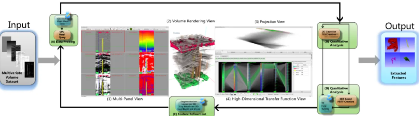
Figure 1: The user interface and the work flow of the system implementing our proposed method. Four closely linked views are shown and labeled, namely: (1) multi-panel view, (2) volume rendering view, (3) projection view and (4) high-dimensional transfer function view. Three stages: (A) data probing, (B) qualitative analysis and (C) optional feature refinement comprise our work flow. With the proposed method and user interface, domain users are able to explore and extract meaningful features in highly complex multivariate dataset, e.g. the 3D seismic survey shown above.
ABSTRACT
Multivariate volumetric datasets are important to both science and medicine. We propose a transfer function (TF) design approach based on user selected samples in the spatial domain to make mul-tivariate volumetric data visualization more accessible for domain users. Specifically, the user starts the visualization by probing fea-tures of interest on slices and the data values are instantly queried by user selection. The queried sample values are then used to au-tomatically and robustly generate high dimensional transfer func-tions (HDTFs) via kernel density estimation (KDE). Alternatively, 2D Gaussian TFs can be automatically generated in the dimension-ality reduced space using these samples. With the extracted features rendered in the volume rendering view, the user can further refine these features using segmentation brushes. Interactivity is achieved in our system and different views are tightly linked. Use cases show that our system has been successfully applied for simulation and complicated seismic data sets.
Index Terms: Computer Graphics [I.3.7]: Three-Dimensional Graphics and Realism—Color, shading, shadowing and tex-ture; Image Processing and Computer Vision [I.4.10]: Image Representation—Volumetric
1 INTRODUCTION
Multivariate dataset visualization has been an active research area for the past decade and is still a challenging topic. A linked-view visualization system that enables the users to explore the datasets
∗e-mail: [email protected] †e-mail: [email protected]
in both the transfer function domain and the spatial domain may boost their understanding of the data. In recent years, visualization researchers have been studying this topic and some solutions have been proposed [6, 1, 4, 10]. These linked-view systems provide users the ability to explore the dataset with closely linked scientific visualization views, e.g., volume rendering or isosurface rendering, and information visualization views, e.g., scatter plots, parallel co-ordinate plots (PCP) or dimensionality reduction views. Typically, the user explores and extracts features of interest by interactively designing transfer functions (TFs) in the value domain over the information visualization contexts and examining classified result in the spatial domain from the scientific visualization view. Suc-cessful examples using these systems are clearly shown for sim-ulation datasets. However, extracting meaningful features in real world measurement datasets, e.g., multi-variate 3D seismic survey, via these systems is not trivial. Features inside the seismic dataset have to be recognized in the spatial domain by a geology expert, and the features have complicated combinations of attribute val-ues and subtle differences from their surroundings. Therefore, it is too laborious to extract features by iterating between TF design in the value domain and getting feedback from the results rendered in the spatial domain, especially when the dimensionality is high. Our geophysicists collaborators have found extracting features with only the value domain TF widgets, e.g. on a PCP to be cumber-some, and specifically asked for more automated methods.
In this paper, we propose a TF design approach based on user selected samples from the spatial domain represented as slices for more intuitive exploration of multivariate volume datasets. Specifi-cally, the user starts the visualization by probing features of interest in a panel view, which simultaneously displays associated data at-tributes in slices. Then, the data values of these features can be instantly and conveniently queried by drawing lassos around the features or, more easily, by applying “magic wand” strokes. High dimensional transfer functions (HDTFs) can then be automatically IEEE Pacific Visualization Symposium 2013
26 February - 1 March, Sydney, NSW, Australia 978-1-4673-4797-6/13/$31.00 ©2013 IEEE
and robustly generated from the queried data samples via the ker-nel density estimation (KDE) [26] method. The TFs are represented by parallel coordinate plots (PCPs) and can be interactively mod-ified in a HDTF editor. Automatically generated Gaussian TFs in dimensionality reduced 2D view can also be utilized to extract fea-tures. The extracted features are rendered in the volume render-ing view usrender-ing directional occlusion shadrender-ing to overcome artifacts from Phong shading in multivariate case. To further refine features, which share similar data value ranges, direct volume selection tools on the volume rendering view or the panel view can be applied.
The contributions of this work are the followings: we propose a transfer function design method for multivariate volume visualiza-tion based on user selected samples, specifically: a HDTF gener-ation method based on KDE and a Gaussian mixture model based 2D Gaussian TF generation method. Second, an interactive multi-variate volume visualization system based on the proposed method that has been implemented to allow domain users to extract refined features in very complicated multivariate volume datasets more in-tuitively.
2 RELATEDWORK Transfer Function Design
Volume datasets can be explored using transfer functions. A 1D TF that uses scalar values of the volume or a 2D TF that has the gradient magnitude of the volume as a second property for better classification [15] are most frequently used. The TFs can be inter-actively defined by 1D TF widgets or 2D TF widgets proposed by Knisset al.[16]. However, to design a good TF, the user has to manipulate the TF widgets in the value space and check result in the volume rendering view which is laborious and time consuming. To address this issue, researchers have proposed to automate the TF generation process. Maciejewskiet al.[19] utilize KDE to structure the data value space to generate initial TFs. Note that instead of per-forming KDE over a 2D value space of the whole data as in [19], our proposed approach applies KDE over samples selected by the user to robustly generate HDTFs. Also focusing on the value space, Wanget al.[28] initialize TFs by modeling the data value space us-ing Gaussian mixture model and render the extracted volume with pre-integrated volume rendering. Our automated Gaussian TFs are similar to their work, however, our working space is created from multidimensional reduction while theirs is traditional 2D TF space. Alternatively, the volume exploration system proposed by Guoet al.[9] allows the user to directly manipulate on the volume ren-dering view with intuitive screen space stroking tools similar to 2D photo processing applications. In contrast to our work, all methods mentioned above work on volumes with only one or two attributes.
Multidimensional Data Visualization
Visualizing and understanding multidimensional datasets has been an active research topic in information visualization. Scat-ter plot matrices, parallel coordinate plots [13] and star-glyphs [29] are common approaches for discrete multidimensional data visu-alization. An efficient rendering [21] method has been proposed to make meaningful and interactive visualization of large multidi-mensional datasets possible. Dimultidi-mensional reduction and projec-tion are other techniques for multidimensional data visualizaprojec-tion. These techniques provide a similarity based overview for multidi-mensional data. Numerous research efforts have been focused on this topic, and popular methods include: principal component anal-ysis (PCA) [14], multidimensional scaling (MDS), isomap [27], and Fastmap [7]. We employ Fastmap due to its speed, stability and simplicity.
Linked View Systems
Multivariate volume datasets can be explored using linked view systems which have shown to be useful for multivariate simulation data exploration. The SimVis system [6, 24] allows the user to inter-act with several 2D scatter plot views using linked brushes to select
features of interest in particle simulations rendered as polygons and particles. Akiba and Ma [1] propose a tri-space exploration tech-nique involving PCPs together with time histograms to help the design of HDTFs for time-varying multivariate volume datasets. Blaaset al. [4] extent parallel coordinates for interactive explo-ration of large multi-time point datasets rendered as isosurfaces. More recently, Zhao and Kaufman [30] combine multi-dimensional reduction and TF design using parallel coordinates but, their system is only able to handle very small datasets. Guoet al.[10] propose an interactive HDTF design framework using both continuous PCPs and multidimensional scaling technique accelerated by employing an octree structure. However, we have observed two limitations in the above systems: 1) the user has to explore the data via interac-tions on the TF view which may be unintuitive for domain users and moreover makes exploration for real-world datasets difficult, and 2) the visualization is merely produced with TFs and it is dif-ficult to achieve a more refined result. As such, we have imple-mented a linked view system that improves on these two issues to allow the domain user to explore complex real-world datasets more intuitively with more refined results.
3 METHODOVERVIEW
The work flow of our proposed method as shown in Figure 1 is comprised of three major stages: (A)data probing, (B)qualitative analysisand (C) optionalfeature refinement. Data probing is the process where the user discovers regions of interest by examining multivariate data slices. The regions of interest can be conveniently selected using lasso tool or “magic wand” tool. Once the regions of interest are selected, a simple, yet efficient, voxel query oper-ation that inquires the multivariate data values is performed. The user then performs a qualitative analysis, i.e., extracting and ren-dering volumetric features by means of designing HDTFs or 2D TFs on dimensionality reduced spaces. KDE is utilized to automat-ically generate the HDTFs and to robustly discard outliers from the queried samples. In addition, automated 2D Gaussian TFs on the projection view offers a simpler alternative for more distinct fea-tures. The HDTFs can then be fine-tuned directly in a PCP based HDTF editor while the 2D Gaussian TFs can be manipulated by 2D Gaussian TF widgets. On many occasions, however, different features share similar data values and thus an optional feature re-finement stage is introduced to refine the features classified by the TFs. Features are refined by the user via segmentation brushes or lassos which are applied directly on the volume rendering view or the multi-panel view.
4 VOXELQUERY ANDPCP GENERATION
Our proposed method is based on user selected multivariate voxel samples through interactive selection which requires efficient voxel query. The multivariate values of the queried samples should be immediately presented to the user by means of PCPs, and as such a fast PCP generation method is needed.
4.1 GPU-based Voxel Query via Conditional Histogram
Computation
Voxel query can be accelerated by spatial hierarchy structures that group similar neighboring voxels into nodes, e.g., an octree struc-ture adopted by Guoet al.[10]. However, Knollet al.[17] report that, “Conversely, volumes with uniformly high variance yield lit-tle consolidation; due to the overhead of the octree hierarchy they could potentially occupy greater space than the original 3D array.” Our initial experiment on the seismic data with the code from [17] agrees with this statement. As such, we propose to efficiently con-duct the voxel query by computing sets of joint conditional his-tograms via a simple GPU-based volume traversal. A joint condi-tional histogram jch(a,b)f of two attributesaandbis a 2D
of voxelsV whose evaluated result from a certain boolean func-tion f(Y⃗(V))(Y⃗(V)being the attribute values ofV) is true. If fis always true, the joint conditional histogram degenerates to an un-conditional joint histogram. Note that the values of user selected samples are queried via an unconditional joint histogram computa-tion over the user selected region on the given slice.
For a multivariate volume of N attributes, given an N-dimensional TF as the condition, a set ofN−1 joint conditional histograms can be computed to record the query results. The values of the joint conditional histograms are accumulated by first evalu-ating theN-dimensional TF for all voxels in the volume, and then transforming the voxels that have positive opacities from the TF into bins in the conditional histogram space, and finally increment-ing the joint conditional histogram count at those bins. Specifically, given a voxelvXofNattributesY1,Y2, ...,YN(to be concise, we use
yito denote the attribute valueYi(vX)) located at 3D positionX in
the spatial domain, and anN-dimensional TFTF. vX→ {(y1,y2),(y2,y3), ...,(yN−1,yN)}
where TF(y1,y2, . . . ,yN).a>0 (1) (y1,y2),(y2,y3), ...,(yN−1,yN) being the bins of joint conditional
histogramsjch(Y1,Y2),jch(Y2,Y3), ...,jch(YN−1,YN)respectively.
Equation 1 and the accumulation of the conditional histograms, which are stored aggregately as a 2D texture array ofN−1 slices, can be easily implemented on the GPU via geometry shader and
ADDblending or read-write textures with atomic operations that are supported on recent GPUs.
4.2 Parallel Coordinate Plots Generation
As proposed in [21], Figure 2 shows that each non-zero pixelP(i,j)
in the joint histogram of attributexandyyields a quad starting at the position ofion PC axisxand ending at the position of jon PC axisy. The highly parallel process can be implemented on the
Figure 2: Generating a PCP from a joint histogram. GPU using geometry shader and transform feedback buffers. The algorithm loops through all pairs of conditional histograms after setting up the transform feedback buffer for recording the resulting geometry. In each iteration, a regular grid of the same size of a slice of the input conditional histogram texturetexcondis drawn and
a geometry shader generates a colored quad for each vertex whose texcond value is not 0. The dynamic range of the data values is
usually high and thus the ratio of natural logarithm of the data value versus natural logarithm of the total voxel number is computed and then modulated with the input colorC0(i,j)at grid position(i,j)to give the final colorC(i,j).
C(i,j) =C0(i,j)log(v(i,j))
log(∑v) (2)
Finally, all quads are stored in the transform feedback buffer, and they can be rendered directly from the transform feedback buffer without being read back to the CPU.
5 TRANSFER FUNCTION GENERATION FROM USER SE
-LECTEDSAMPLES
In this section, the actual TF generation method will be explained. Section 5.1 introduces the method for interactive voxel sample se-lection, Section 5.2 discusses the KDE based HDTF generation method and Section 5.3 details on the automated 2D Gaussian TF on the dimensionality reduced space.
5.1 Sample Selection in the Multi-panel View
The user can interactively select arbitrary a region of interest in any attribute by either drawing a lasso or using the magic wand tool. The lasso tool is a simple free hand drawing tool which allows the user to select regions by manually drawing over the boundary of a feature. Although very flexible, the user has to be very careful when drawing on the boundary using the lasso tool.
To alleviate the difficulty of perfectly drawing over the boundary of a feature, a more intuitive and easier to use magic wand tool is introduced. The magic wand tool is essentially a 2D segmentation tool based on Perona and Malik anisotropic diffusion [23]. Equa-tion 3 describes the diffusion equaEqua-tion whereS(t,x,y)is the number of seeds at position(x,y)at timet,V(t,x,y)being the intensity of the chosen attribute at the same point,|∇V(t,x,y)|is its gradient magnitude, andg(s)being a conductivity term.
∂S(t,x,y)
∂t =div(g(|∇V(t,x,y)|)∇S(t,x,y)) (3) whereg(s) =v·exp−s
2
K2
ParameterKgoverns how fastg(s)goes to zero for high gradients, regular termvis chosen as 1 and normalization termhis set to
1
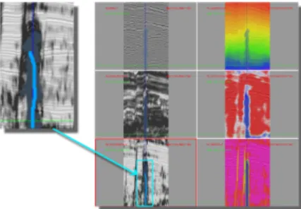
n+1 for numerical stability,nbeing the number of neighbors of a pixel which is 8 in our case. Equation 3 can be solved numerically using the finite difference method with a given iteration numberT. The iteration numberT, parameterK and seeding brush size are user controllable. Figure 3 shows the panel view of a six-attribute seismic volume dataset where attributes are co-rendered with the seismic amplitude volume. Note that a user drawn magic wand in dark blue highlights a potential salt dome structure.
Figure 3: The user draws on a salt dome (stroke shown in light blue) over the fifth attribute in the panel view resulting in the dark blue region of selection.
5.2 Kernel Density Estimation based Transfer Function Generation
We would like to generate HDTFs from the samples selected us-ing method described in Section 5.1. To reduce the computational complexity, we separate theN-dimensional value space intoN−1 2D value spaces, i.e. a 2D+2D+···+2D(N−1 of 2D) space. A naive approach is to generate a TF by taking the convex hull of these 2Dsample points. Although useful when the user intents to select exact sample points, it is conceivable that the outliers in the samples can greatly bias the generated TF and result in unwanted regions selected in the value space.
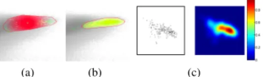
Figure 4(a) clearly demonstrates such a situation where a red 2D TF widget is generated as the convex hull of the sample points with the red boundary. Also notable is that the color gradient of the TF widget is arbitrarily defined by the user that may not follow the underlying distribution of data.
Kernel density estimation (KDE) [26] seen in Equation 4 is a non-parametric method for estimating the density functionfh(x)at
(a) (b) (c)
Figure 4: User selected sample points (shown in green) over a joint histogram. TF widget generated from the samples as (a) convex hull and (b) KDE. In (c): a point cloud (left) and its KDE result color coded with a ’jet’ color map.
locationxof an arbitrary dimensional domainΩwith given samples
{xi},i∈ {1,2,3, . . . ,n}. fh(x) = 1 n n
∑
i=1 Kh(x−xi) = 1 nh n∑
i=1 K(x−xi h ),x,xi∈Ω (4) where K(x) being the kernel function and h is the bandwidth. Thanks to the separation of the value space, instead of computing the KDE forΩofNdimension, we computeN−1 KDE forΩin 2D spaces. In our case, eachΩis set to the same size of the 2D joint histogram which is typically 256×256. An empirical optimal bandwidth estimator is suggested in [26], which can be extended to 2D:h=1.06√detΣ·n−15 (5)
where detΣis the determinant of the 2Dcovariance matrixΣof current attribute pairs. The kernel functionK(x)we used is the 2D Gaussian kernel:
K(x) =√1
2πe −||x||2
2 (6)
With the Gaussian kernel, each samplexicontributes to the estimate
in accordance with its distance fromx. Therefore, in the region near the intended samples more short distanced samples are contributing to fh(x)compared to the region near outliers. As a result, the
den-sity valuefh(x)around the outliers is lower than that of the intended
samples.
Figure 4(c) shows the density function generated by the KDE method of the given samples with the above settings. It verifies our expectation that the outliers have lower density than the intended sample regions. As such, we can discard the outliers by setting a threshold for the density value fh(x). Figure 4(b) shows the yellow
TF widget generated by KDE with a density threshold of 0.15. No-ticeable is that the outliers are excluded from the TF widget and the smooth color gradient that actually follows the underlying density. The resulting TF can be represented by a set of 2D TFs or a PCP created using the method described in Section 4.2.
In the presence of multiple HDTFs, ambiguity could arise: dif-ferent HDTFs can cover the same regions of certain 2D attribute pairs. To differentiate the HDTFs, a unique ID is specified to each HDTF and an ID map of the same size of theN−1 2D TF space is created by conducting bitwiseORfor all HDTFs on each 2D at-tribute pair. The ID map is later decoded in the volume rendering shader to correctly select voxels.
5.3 Automated Gaussian Transfer Functions on
Dimen-sionality Reduced Space
Dimensional reduction is another popular method for visualizing high dimensional data due to its ability to intrinsically generate vi-sual representations that are easy to understand and interact with. Instances in anm-dimensional Cartesian space are projected into a lowerp-dimensional visual space with preservation of the distances
between instances as much as possible. In other words, voxels with similarm-dimensional attribute values are projected to be near each other in the p-dimensional space. With a projected visual space of p=2, the user is able to better identify features by doing vi-sual classification using a 2D TF widget, and moreover, automated clustering methods can be applied for classification. In our pro-posed method, the high-dimensional value space is projected into a 2D space using Fastmap [7] and then Gaussian TFs are generated via expectation maximization optimization with Gaussian mixture model. The user can choose to use either the 2D Gaussian TF or the HDTF for each feature by switching a button on the user interface. The 2D Gaussian TFs are preferred for more convenient extraction of several distinct features at the same time, while the HDTFs are better for features that have subtle differences in the HD value do-main.
5.3.1 Dimensional Reduction using Fastmap
We employ Fastmap [7] as the dimensional reduction technique since it is fast, stable and easy to implement. Fastmap is a recur-sive algorithm for multidimensional projection with anO(N)time complexity. Given target dimensionk, a distance functionD()and object arrayOcontainsN objects ofmdimension, the algorithm
FastMapcomputes thekdimensional projected imageXfrom the
Nobjects. The algorithm can be summarized as the following: FastMap(k,D(),O)
ifk≤0then return else
col=col+1 (colis initialized to 0)
end if
Choose and record the pair of pivot objectsOa,Ob. Project objects on line(Oa,Ob)using the cosine law:
X[i,col] =xi=D(Oa,Oi) 2+D(Oa,Ob)2−D(Ob,Oi)2 2D(Oa,Ob) ,i∈ {0,1,2, ...,N−1} Call FastMap(k−1,D′(),O). Where D′(O′i,O′j)2=D(Oi,Oj)2−(xi−xj)2,i,j∈ {0,1,2, ...,N−1}
5.3.2 Gaussian Mixture Model with Expectation
Maximiza-tion
Assuming that all attributes we are handling are continuous mea-surements, the dimensionality reduced 2D value space can therefore be modeled by a Gaussian mixture model (GMM). GMM models point clouds by assigning each cluster a Gaussian distribution. For a pointxin the 2D value space, a Gaussian distribution is shown in Equation 7 with mean valueµbeing a 2D vector and covariance matrixΣas a 2×2 matrix.
N(x|µ,Σ) = 1
2π|Σ|1/2e−
1
2(x−µ)TΣ−1(x−µ) (7)
Therefore, for a GMM withkcomponents, the distribution of the 2D value space can be written as
p(x|θ) = k
∑
j=1
αjN(x|µj,Σj) (8)
where θ is the parameter set of the k-component GMM
{αj,µj,Σj}k
j=1, andαj is the prior probability of the jth Gaus-sian distribution. The optimal ˆθcan be found asθthat maximizes the likelihood ofp(X|θ)
ˆ
θ=arg maxp(X|θ) =arg max
n
∏
i=1
wherenis the number of input points. Equation 9 can be solved by the expectation maximization (EM) algorithm [3]. Given an initial setup ofθ, the EM algorithm iterates between two steps: expec-tation step (E step) and maximization step (M step) until the log likelihood lnp(X|θ) =log( n
∏
i=1 p(xi|θ)) = n∑
i=1 {∑
k j=1 αj N(xi|µj,Σj)} converges.We initialize the EM algorithm using the K-means algo-rithm [12] which quickly gives a reasonable estimation ofθ. With an initialization ofkmean values{µj}kj=1, K-means algorithm iter-atively refines{µj}kj=1until convergence through assignment and update steps. The assignment step assigns each sample to the clus-ter with the closest mean, and the update step calculates the new means to be the centroid of each cluster. In our case, the initial means arekrandom samples in the input dimensional reduced 2D point cloud. Once the K-means algorithm terminates,{Σj}k
j=1can be easily computed with the result means, and prior probabilities
{αj}k
j=1 is given by the proportion of total samples inside each cluster.
5.3.3 Automated 2D Gaussian Transfer Functions
We use a modified TF generation scheme as in [28] but ours differs in 1) the value space we use is the 2D dimensionality reduced space of high-dimensional attribute compared to the 2D intensity versus gradient magnitude space as in [28], and 2) we use the user selected samples as the input point clouds while they use all voxels in a volume.
Given some user provided sample data points and a class num-berk(which is set to 3 by default from our experiments), the EM algorithm computes the Gaussian distribution parameters ˆθ. Each Gaussian distribution is managed by a Gaussian TF widget with a user defined colorCand opacity functionαof locationx:
α=αmaxe−12(x−µ)
TΣ−1(x−µ)
(10) The Gaussian TF widget is centered at the mean valueµ of the Gaussian distribution and its boundary is generated by transforming a unit circle with the square root matrixΣ1/2of covariance matrix Σ.Σ1/2is calculated via eigen decomposition ofΣ:
Σ=V DV−1 (11)
Σ1/2=V D1/2V−1 (12) whereDis a diagonal matrix holding the eigen values andV con-tains the eigen vectors as columns.V is an orthogonal matrix, i.e. V−1=VT, sinceΣis symmetric. The eigen valuesσ1,σ2are the radii of the principal axes of the ellipse, while the eigen vectorsa,b are the unit vectors of the principal axes.
Transformations of the Gaussian widgets, i.e. translation, rota-tion and scaling, can be achieved using the eigen values and eigen vectors. The translation is done by shifting theµwith an offset∆µ given by user dragging. The rotation of the widget is achieved by rotating the eigen vectors inVwith an angleβ. Finally, multiplying the eigen valuesσ1,σ2with a scaling factor(sa,sb)results in the
scaling of the widget.
6 FEATUREREFINEMENT INTHESPATIALDOMAIN
The feature refinement stage is introduced to allow the user to di-rectly manipulate the features in the spatial domain. Various refine-ment tools have been implerefine-mented to handle different situations. All tools support three refinement modes: new, add and remove.
(a) (b) (c)
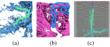
Figure 5: Feature refinement tools: (a) 3D brush, (b) 3D lasso and (c) 2D brush.
Screen Space Brush in the 3D View. The tool as seen in Fig-ure 5(a) allows the user to draw strokes on the 3D view screen to set seeds in the visualization results, and then a GPU based region growing is conducted to set the connected voxels to a given tag number. The seeding location is determined by casting rays from brush strokes on the image plane to the volume extracted by current TFs. A voxel along the ray is seeded when its opacity is greater than a user defined threshold.
Screen Space Lasso in the 3D View.Alternatively, the user can directly indicate features of interest on the 3Dview using a lasso as shown in Figure 5(b). A lasso is a simple tool that selects all voxels from the TF extracted volume that are inside the back projected volume of the screen space lasso covered area.
Refinement Brush in the Panel View.The refinement can also be done by seeding on the panel view via drawing strokes (Fig-ure 5(c)), and this is useful when the feat(Fig-ures of interest are oc-cluded in the 3D view or readily visible in a slice.
A morphological closing, i.e. dilate the volume by one voxel and then erode the volume by one voxel, is performed after refinement in order to fill small holes and bridge tiny gaps. Note that all refined feature groups are managed in the group manager in the HDTF ed-itor introduced in section 8.2, and thus similar to TF groups, their colors can be changed, they can be deleted and their visibility can be toggled.
7 RENDERING
We employ the directional occlusion shading (DOS) [25], which is an efficient approximation to ambient occlusion as the render-ing technique because that the DOS is gradient-free and provides the user more insights into the dataset than local shading models as shown on seismic datasets [22]. A user study conducted by Linde-mann and Ropinski [18] shows that DOS outperforms other state-of-the-art shading techniques in relative depth and size perception correctness. Hardware supported trilinear interpolation cannot be used for tag volume rendering because false tag values will be generated. Instead, nearest neighbor sampling has to be used to correctly render the tag volume. However, a simple use of near-est neighbor sampling yields blocky looking results because of the voxel level filtering. Instead, using a manual trilinear 0-1 interpo-lation gives pixel level filtering. From our observations, the cases where multiple tags appear in a single 8 voxel neighborhood rarely occur and as such a simplified method of [11] is utilized. The largest tag value in the eight neighboring voxels around current pixel is mapped to 1 and all others to 0 and then a trilinear inter-polation is conducted on these 0/1 values. The interpolated result is then compared against 0.5, if greater, the final tag value of the pixel is set to the pixel’s nearest neighboring voxel’s tag value, otherwise the tag value is set to 0.
8 USERINTERFACE
The user interface of our system is seen in Figure 1 where a multi-panel slice view for data probing is shown to the left (1), an interac-tive 3D view that shows volume rendering results and allows post feature manipulation is seen in the middle (2), a projection view
shown to the upper right (3) and a high dimensional transfer func-tion view appears to its bottom (4). These four views are tightly linked and as such any updates in one view will be reflected in oth-ers.
8.1 Multi-panel Viewer
We have developed a multi-panel view which shows all attributes of a slice by placing attributes into individual panels as seen in the left part of Figure 1 as well as in Figure 3. The multi-panel viewer synchronizes user interactions across all attribute views including: mouse positioning, panning, zooming, scrolling and aspect chang-ing. To enhance the perception of attributes, each attribute can have a specifically designed color map that highlights features of interest. In order to better use the dynamic range of the color maps, the con-trast of the attributes can be conveniently changed using the mouse wheel. Furthermore, a background volume can be co-rendered with the current attribute volume using transparency. This is especially helpful for seismic volumes as our collaborating geologists suggest that it provides more insight into the attributes when the seismic amplitude volume is co-rendered as a context.
8.2 HDTF Editor
The user can interact with the HDTF editor to manually modify the HDTFs. Figure 6 shows the HDTF editor where the PCP axes reorder button and attribute-wise control panel can be seen on the top, the PCP TF editor is seen in the upper left, a group manager is shown to its right while the pair-wise TF editor is shown in the lower part. The attribute-wise control buttons allow the user to specify a color map, toggle sampling between linear and nearest neighbor, and toggle lock/unlock for each attribute. A locked at-tribute is essentially an atat-tribute with its entire value range used in TFs, in other words, it can be visualized in the panel view but is not contributing to classification. This is useful since not all at-tributes provide positive assistance in the extraction of specific fea-tures and this knowledge is usually not known before hand. Also, there are cases when one needs an attribute to provide only con-text for data probing, e.g. the seismic amplitude attribute which will be discussed in Section 9. The group manager manages all TF and segment groups. One is able to toggle the visibility or remove individual or a batch of groups conveniently.
Figure 6: The HDTF editor. Note that the first attribute, seismic amplitude, is locked.
As seen in Figure 6, the PCP axes are co-rendered with the 1D histograms of attributes shown to the right and color map to the left. Since the color map is synchronized with the one that appears in the panel view, the user is able to instantly know how to set the TF widgets. The user interacts directly with the parallel coordinate axes to design an HDTF using one of the three interaction widgets, namely:brush widget,tent widgetandGaussian widget. The brush widget enables the user to arbitrarily interact with the TF domain.
Tent and Gaussian widgets are essentially sets of 1D TF widgets residing on each attribute axis of the HDTF domain, and they differ only in their shape of opacity gradient.
In addition to the PCP TF editor, a pair-wise 2D TF editor is used to aid the exploration of pair-wise features. The pair-wise 2D TF editor allows the user to interact withN−1 2D TF space to fine tune the HDTFs to match irregular shaped features in specific pairs of attributes using 2D rectangle, triangle or lasso widgets. 8.3 Projection Viewer
A projection viewer has been implemented in our proposed system by combining the Fastmap dimensional reduction technique with GMM 2D Gaussian TFs. The projection viewer extends the tradi-tional 2D TF editor with Gaussian TF widgets, but preserves famil-iar 2D TF widgets: rectangle, triangle and lasso. Closely linked with the panel view and the HDTF editor, the projection viewer shows the dimensional reduction view of user selected samples. 9 USECASES
Two use cases from different application domains will be shown to demonstrate the usefulness of our proposed method. The first case is a commonly used hurricane simulation data set and the second case is a 3D seismic survey data with several derived attributes, which will be used to extract geological features that are important in the petroleum industry since they indicate potential oil and gas reservoirs.
9.1 Hurricane Isabel Simulation
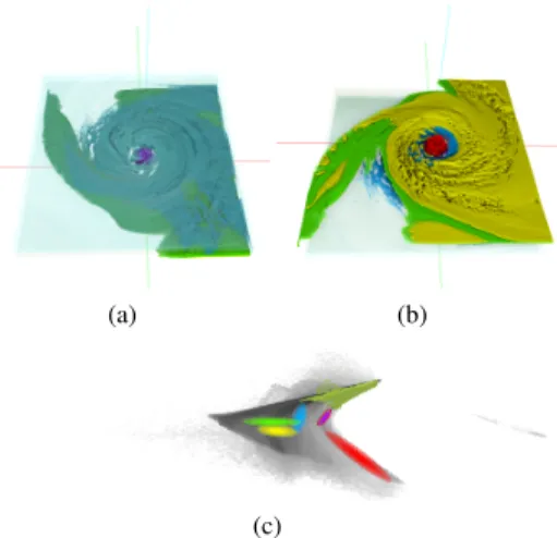
We have experimented with the proposed system on the simula-tion dataset: hurricane Isabel. The hurricane Isabel dataset, intro-duced by IEEE visualization contest 2004, is a multivariate multi-ple time step atmospheric simulation data. Eight attributes of time step 25 are used to generate the result in Figure 7, namely the pres-sure, the temperature, the total precipitation mixing ratio (PRECIP), the graupel mixing ratio (QGRAUP), the water vapor mixing ratio (QVAPOR), the total cloud moisture mixing ratio(CLOUD), and the speed. The simulation dataset contains no noise and since each
(a) (b)
(c)
Figure 7: The extracted features shown in (a) the top view and (b) the bottom view. Seen in (c) is the corresponding projection view with automated Gaussian TFs that produce the classification result. attribute represents a clear physical meaning, it is relatively easy to classify. A good classification can be achieved by HDTFs or alter-natively by automated 2D Gaussian TFs on the projection view as seen in Figure 7. Joint histograms could be generated with contin-uous scatter plots [2]. The user can generate the result in Figure 7 by placing several large lassos on slices in the axial view (slices
indexed by the z axis) on the multi-panel viewer in the data prob-ing stage. The GMM-EM algorithm explained in section 5.3 then automatically generates the TFs for classification in the qualitative analysis stage. The hurricane eye, spiral arms and the top of the atmosphere are clearly seen in Figure 7. Due to the nature of this data, no feature refinement is required.
The results are similar compared to previous methods. With pre-vious methods [6, 1, 4, 10], one has to carefully design the TFs one by one for each feature, either by editing pairs of histograms [6], or PCP-based HDTF [1, 4] or high-dimensional Gaussian TF and MDS-based TF [10]. Our method, however, allows the user to ex-tract the same features by simply drawing several large lassos across the features on the multi-panel viewer, which is significantly eas-ier.
9.2 3D Seismic Dataset
3D seismic imaging has been the standard for oil and gas explo-ration for decades, and more recently, multi-attribute volumes de-rived from the seismic amplitude volume have been used to aid the understanding of the seismic surveys [5]. However, these derived volumes are visualized individually in current seismic data analy-sis tools and as such the relationships between attributes are lost. With the proposed methods and our system, our collaborating geo-physicists successfully extract refined geological features from the dataset and can export the results as a labeled volume for further processing.
The data used is a part of the public 3D seismic survey dataset “New Zealand” of size 213×276×426, in which different geo-logical features exist, including channels, faults, and a salt dome, that can be potential reservoirs of oil and gas. Five attributes have been derived from the original seismic amplitude data (Amp). Us-ing the six attributes, namelyAmp,Seg MedFilter,Inst Amp,
Inst Phase Entropy,SembandSemb Thick, geophysicists
are able to clearly extract meaningful features as shown in Fig-ure 8. Note that for all featFig-ures,Ampprovides only context and is
Figure 8: Extracted geological features: a shallow channel com-plex in red, a salt dome shown in yellow, a deeper channel shown in purple and the largest fault in green.
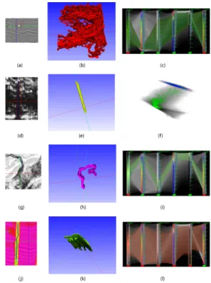
not clamped in order to select complete geological structures. The geophysicist starts the exploration by scrolling through the slices in the inline direction (slices indexed by the xaxis) and finds a shallow channel complex in theAmp. In the data probing stage, a lasso around the channel complex is drawn on theAmpattribute seen in Figure 9(a), from this an HDTF is generated with the KDE method described and fine tuned in the qualitative analysis stage as shown in Figure 9(c). The main connected component as shown in Figure 9(b) is extracted in the feature refinement via segmentation brushing in the 3D view.
The salt dome appears to be a distinct feature on slices in the cross line direction (slices indexed by theyaxis) and as such the
automated Gaussian TFs in the projection view are utilized. By drawing a lasso around the salt dome on theInst Ampattribute, as shown in Figure 9(d), Gaussian TFs are automatically gener-ated in the projection view. The visualization of the isolgener-ated salt dome seen in Figure 9(e) is created by enlarging the Gaussian wid-get (Figure 9(f)) that highlights the salt dome and drawing a region growing brush stroke on the salt dome.
Scrolling down through the time direction (slices indexed byz axis), a smaller channel is discovered at the bottom of the volume. The lower channel is clearly visible in theInst AmpandSemb
attributes. Using the magic wand tool inside the channel on the
Inst Ampattribute (Figure 9(g)), and fine tuning the HDTF as
seen in Figure 9(i), the channel can be extracted. Due to its connec-tion to the surroundings, we use the lasso tool to manually extract only the channel as shown in Figure 9(h).
Finally, when the geophysicist switches back to the inline direc-tion, the faults are easily recognized in theSemb Thickattribute and are partly extracted via magic wand brushing (Figure 9(j)). Since that the faults depend only on the Semb Thickattribute, it is fine tuned to cover the entirety of the faults (Figure 9(l)). The largest fault as seen in Figure 9(k) is extracted via region growing brushing in the 3D view. In theory, previous methods that use only the value domain TF widgets are able to extract the features. How-ever, our collaborating geophysicists have found that in practice, it becomes overwhelmingly laborious.
Figure 9: Refined features shown in the middle column with the user’s selection of regions of interest shown in the left column, and their TFs shown to the right. Note that the color of the refined features are independent of their TF colors.
10 IMPLEMENTATION
The system is implemented in C++ with OpenGL and Qt. The magic wand tool, conditional histogram generation, PCP cre-ation and region growing based segmentcre-ation are accelerated us-ing GLSL shaders. Directional occlusion for volume renderus-ing and PCP rendering are implemented on the GPU as well. The
figtreepackage [20] is utilized for efficient kernel density es-timation. The linear algebra operations are aided by theEigen
library [8].
11 CONCLUSION ANDFUTUREWORK
We have presented a TF design method to provide a more intuitive multivariate volume exploration experience with refined feature ex-traction results. An interactive system is built to realize these pro-posed methods. Results from the multi-attribute hurricane simula-tion and 3D seismic survey data sets demonstrate that the system is able to extract features in both commonly used simulation data and highly complicated real-world data. The applications are domain dependent and require domain knowledge, thus our tool is interac-tive and empirical, and our collaborating geophysicists found merit in the system.
For future work, we would like to further develop our system in three ways: 1) improve the scalability, 2) further reduce the user’s workload using advanced machine learning methods, and 3) sup-port time varying datasets. GPU-based out-of-core methods for volume rendering, conditional histogram computation and PCP ren-dering could support full size 3D seismic data. The user interaction of the system is intuitive as reported by the geophysicists, but is still time consuming for very complicated data sets. By introducing ad-vanced machine learning methods, we hope to make the interaction more automated, e.g. an appropriate slice that captures useful fea-tures can be automatically found for the user. Our work can now be applied only to one time step of a simulation. However, thanks to the temporal coherence between the simulation steps, and the user defined TFs on one time step can be propagated to other time steps with incremental update methods.
ACKNOWLEDGEMENTS
This research was sponsored by the DOE NNSA Award DE-NA0000740, KUS-C1-016-04 made by King Abdullah Univer-sity of Science and Technology (KAUST), DOE SciDAC Insti-tute of Scalable Data Management Analysis and Visualization DOE DE-SC0007446, NSF OCI-0906379, NSF IIS-1162013, NIH-1R01GM098151-01.
REFERENCES
[1] H. Akiba and K.-L. Ma. A tri-space visualization interface for ana-lyzing time-varying multivariate volume data. InProceedings of Eu-rographics/IEEE VGTC Symposium on Visualization, pages 115–122, May 2007.
[2] S. Bachthaler and D. Weiskopf. Continuous scatterplots.IEEE Trans-action on Visualization and Computer Graphics, 14(6):1428 –1435, nov.-dec. 2008.
[3] J. Bilmes. A gentle tutorial of the EM algorithm and its application to parameter estimation for Gaussian mixture and hidden Markov mod-els. Technical Report TR-97-021, ICSI, 1997.
[4] J. Blaas, C. Botha, and F. Post. Extensions of parallel coordinates for interactive exploration of large multi-timepoint data sets. IEEE Transactions on Visualization and Computer Graphics, 14(6):1436 – 1451, nov.-dec. 2008.
[5] S. Chopra and K. J. Marfurt. Seismic Attributes for Prospect ID and Reservoir Characterization (Geophysical Developments No. 11). So-ciety Of Exploration Geophysicists, 2007.
[6] H. Doleisch. Simvis: interactive visual analysis of large and time-dependent 3d simulation data. InProceedings of the 39th confer-ence on Winter simulation, WSC ’07, pages 712–720, Piscataway, NJ, USA, 2007. IEEE Press.
[7] C. Faloutsos and K.-I. Lin. Fastmap: a fast algorithm for indexing, data-mining and visualization of traditional and multimedia datasets. SIGMOD Rec., 24(2):163–174, May 1995.
[8] G. Guennebaud, B. Jacob, et al. Eigen v3. http://eigen.tuxfamily.org, 2010.
[9] H. Guo, N. Mao, and X. Yuan. Wysiwyg (what you see is what you get) volume visualization. IEEE Transactions on Visualization and Computer Graphics, 17(12):2106–2114, Dec. 2011.
[10] H. Guo, H. Xiao, and X. Yuan. Multi-dimensional transfer function design based on flexible dimension projection embedded in parallel coordinates. InPacific Visualization Symposium, 2011.
[11] M. Hadwiger, C. Berger, and H. Hauser. High-quality two-level vol-ume rendering of segmented data sets on consvol-umer graphics hardware. InVisualization, 2003. VIS 2003. IEEE, pages 301 –308, oct. 2003. [12] J. A. Hartigan and M. A. Wong. Algorithm as 136: A k-means
clus-tering algorithm. Journal of the Royal Statistical Society. Series C (Applied Statistics), 28(1):pp. 100–108, 1979.
[13] A. Inselberg. The plane with parallel coordinates. The Visual Com-puter, 1:69–91, 1985.
[14] I. T. Jolliffe.Principal Component Analysis (Springer Series in Statis-tics). Springer, 2002.
[15] G. Kindlmann and J. Durkin. Semi-automatic generation of transfer functions for direct volume rendering. InIEEE Symposium on Volume Visualization, pages 79–86, 1998.
[16] J. Kniss, G. Kindlmann, and C. Hansen. Multidimensional transfer functions for direct volume rendering. IEEE Transactions on Visual-ization and Computer Graphics, 8(3):270–285, 2002.
[17] A. Knoll, I. Wald, S. Parker, and C. Hansen. Interactive isosurface ray tracing of large octree volumes. InInteractive Ray Tracing 2006, IEEE Symposium on, pages 115 –124, sept. 2006.
[18] F. Lindemann and T. Ropinski. About the influence of illumination models on image comprehension in direct volume rendering. IEEE Transactions on Visualization and Computer Graphics, 17(12):1922 –1931, dec. 2011.
[19] R. Maciejewski, I. Woo, W. Chen, and D. Ebert. Structuring feature space: A non-parametric method for volumetric transfer function gen-eration.IEEE Transactions on Visualization and Computer Graphics, 15(6):1473–1480, Nov. 2009.
[20] V. I. Morariu, B. V. Srinivasan, V. C. Raykar, R. Duraiswami, and L. S. Davis. Automatic online tuning for fast gaussian summation. In Advances in Neural Information Processing Systems (NIPS), 2008. [21] M. Novotny and H. Hauser. Outlier-preserving focus+context
visu-alization in parallel coordinates. IEEE Transactions on Visualization and Computer Graphics, 12(5):893 –900, sept.-oct. 2006.
[22] D. Patel, S. Bruckner, I. Viola, and E. Groller. Seismic volume visu-alization for horizon extraction. InPacific Visualization Symposium (PacificVis), 2010 IEEE, pages 73 –80, march 2010.
[23] P. Perona and J. Malik. Scale-space and edge detection using anisotropic diffusion.IEEE Transactions on Pattern Analysis and Ma-chine Intelligence, 12(7):1364–1371, 1990.
[24] H. Piringer, R. Kosara, and H. Hauser. Interactive focus+context visu-alization with linked 2d/3d scatterplots. InCoordinated and Multiple Views in Exploratory Visualization, 2004. Proceedings. Second Inter-national Conference on, pages 49 – 60, july 2004.
[25] M. Schott, V. Pegoraro, C. D. Hansen, K. Boulanger, and K. Boua-touch. A directional occlusion shading model for interactive direct volume rendering.Computer Graphics Forum, 28(3):855–862, 2009. [26] B. W. Silverman.Density Estimation for Statistics and Data Analysis.
Chapman & Hall/CRC, 1986.
[27] J. B. Tenenbaum, V. de Silva, and J. C. Langford. A Global Geo-metric Framework for Nonlinear Dimensionality Reduction. Science, 290(5500):2319–2323, Dec. 2000.
[28] Y. Wang, W. Chen, J. Zhang, T. Dong, G. Shan, and X. Chi. Efficient volume exploration using the gaussian mixture model. IEEE Trans-actions on Visualization and Computer Graphics, 17(11):1560–1573, Nov. 2011.
[29] M. O. Ward. Xmdvtool: integrating multiple methods for visualizing multivariate data. InProceedings of the conference on Visualization ’94, VIS ’94, pages 326–333, Los Alamitos, CA, USA, 1994. IEEE Computer Society Press.
[30] X. Zhao and A. Kaufman. Multi-dimensional reduction and transfer function design using parallel coordinates. InVolume Graphics 2010, IEEE/EG International Symposium on, pages 69–76, may. 2010.