Does lockdown policy reduce human activity?
著者
Souknilanh Keola, Hayakawa Kazunobu
権利
Copyrights 2020 by author(s)
journal or
publication title
IDE Discussion Paper
volume
800
year
2020-09
INSTITUTE OF DEVELOPING ECONOMIES
IDE Discussion Papers are preliminary materials circulated to stimulate discussions and critical comments
* Senior Research Fellow, Economic Geography Studies Group, Development Studies Center, IDE ([email protected])
IDE DISCUSSION PAPER No. 800
Does Lockdown Policy Reduce
Human Activity?
Souknilanh KEOLA and Kazunobu
HAYAKAWA*
September 2020
Abstract: In this study, we empirically investigate how much human economic and social activity was decreased by the implementation of lockdown policy during the coronavirus disease 2019 (COVID-19) pandemic. We measure the magnitude of human activity using nitrogen oxide (NOx) emissions. Our observations include daily NOx emissions in 173 countries between January 1 and July 31, 2020. Our findings can be summarized as follows. Lockdown policy significantly decreased NOx emissions in low-income countries during the policy as well as post-policy periods. In high-income countries, however, NOx emissions increased during both periods. It was also found that the absolute impact of the lockdown policy was larger during the post-policy period than during the policy period. While the stay-at-home policy reduced NOx emissions, we did not discover robust differences between regions in its effect.
Keywords: Coronavirus disease 2019 (COVID-19); Nitrogen Oxide (NOx); Lockdown policy
The Institute of Developing Economies (IDE) is a semigovernmental, nonpartisan, nonprofit research institute, founded in 1958. The Institute merged with the Japan External Trade Organization (JETRO) on July 1, 1998.
The Institute conducts basic and comprehensive studies on economic and related affairs in all developing countries and regions, including Asia, the Middle East, Africa, Latin America, Oceania, and Eastern Europe.
The views expressed in this publication are those of the author(s). Publication does not imply endorsement by the Institute of Developing Economies of any of the views expressed within.
INSTITUTE OF DEVELOPING ECONOMIES (IDE), JETRO 3-2-2, WAKABA,MIHAMA-KU,CHIBA-SHI
CHIBA 261-8545, JAPAN
©2020 by author(s)
No part of this publication may be reproduced without the prior permission of the author(s).
1
Does Lockdown Policy Reduce Human Activity?
§Souknilanh KEOLA Kazunobu HAYAKAWA#
Development Studies Center, Institute of Developing Economies, Japan
Abstract: In this study, we empirically investigate how much human economic and social activity was decreased by the implementation of lockdown policy during the coronavirus disease 2019 (COVID-19) pandemic. We measure the magnitude of human activity using nitrogen oxide (NOx) emissions. Our observations include daily NOx emissions in 173 countries between January 1 and July 31, 2020. Our findings can be summarized as follows. Lockdown policy significantly decreased NOx emissions in low-income countries during the policy as well as post-policy periods. In high-low-income countries, however, NOx emissions increased during both periods. It was also found that the absolute impact of the lockdown policy was larger during the post-policy period than during the policy period. While the stay-at-home policy reduced NOx emissions, we did not discover robust differences between regions in its effect.
Keywords: Coronavirus disease 2019 (COVID-19); Nitrogen Oxide (NOx); Lockdown policy
JEL Classification: F15; F53
Suggested Running Head: Does Lockdown Reduce Human Activity?
1.
Introduction
People have stayed at home since the outbreak of the coronavirus disease 2019 (hereafter, COVID-19) pandemic in early 2020. Many countries imposed restrictions on people and businesses to prevent its further spread. Several countries declared citywide or nationwide lockdowns. Two typical policy measures implemented in response to the pandemic include the workplace-closing policy, which requires all but essential workplaces (e.g., grocery stores) to be shut down, and the stay-at-home policy, whichrequires people not leave their homes except for daily exercise, grocery shopping, and “essential” trips. Beginning in April 2020, many countries introduced such “lockdown” policies, which contributed to decreasing the number of confirmed COVID-19 cases (Ullah and Ajala, 2020; Askitas et al., 2020; Ghosh, 2020) and the number of deaths (Conyon et al., 2020). However, due to lockdown policy, economic activity was substantially suspended worldwide. At the
§ We would like to thank Kyoji Fukao, Shujiro Urata, Hitoshi Sato, Satoru Kumagai, and the seminar
participants in the IDE-JETRO for their invaluable comments. This work was supported by JSPS KAKENHI Grant Number #18H03637. All remaining errors are ours.
# Corresponding author: Kazunobu Hayakawa; Address: Wakaba 3-2-2, Mihama-ku, Chiba-shi, Chiba,
2
expense of the economy, lockdown policy seemed to decrease the spread of the COVID-19. In this study, we quantify the reduction in economic and social activity caused by lockdown policy. We measure the magnitude of human activity using the nitrogen oxide (NOx) emissions, which are remotely sensed using the TROPOspheric Monitoring Instrument (TROPOMI). The TROPOMI is mounted on the Sentinel 5P satellite, which was put into orbit by the European Space Agency (ESA) in 2017. One advantage of this measure is that the near real-time data are provided almost instantaneously with a spatial resolution of approximately 7 km by 7 km. We aggregate these data by country. The major sources of NOx include fuel burning by vehicles, thermal power plants, factories, and residential activity. Therefore, more economic activity will result in the burning of more fuel and thereby more NOx emissions. Many studies have discovered that rain reduces the level of air pollutants by washing them to the ground, indirectly reducing the level of mobility on the roads (e.g., Guo et al., 2016; Kwak et al., 2017). Overall, NOx emissions is related to human economic and social activity.
Using this measure, we examine the effects of the workplace-closing and stay-at-home policies on NOx emissions on a country-daily level. We compare the difference in NOx emissions between periods with and without lockdown policy. Furthermore, for the period without lockdown policy, we differentiate between the pre- and post-policy periods. This analysis is based on the expectation that human behavior might change after experiencing lockdown. Many countries have attempted to sustain economic activity by introducing telecommuting systems. However, the feasibility of such remote work operations differs according to the labor intensity of industries and information technology (IT) development. Thus, to reveal the differences in the effect of lockdown policy between countries, we examine the effect separately for high- and low-income countries. Similarly, we also compare the effect between continents. The number of COVID-19 deaths is mysteriously lower in Asia than in other regions. Due to the relatively less serious situation in Asia, the effect of lockdown policy might differ between continents. Lastly, we examine the effects of other policy measures, including school closures and foreigner entry bans.
Our findings can be summarized as follows. We discovered differences in the effect of lockdown policy according to income level and the study period. Specifically, the workplace-closing policy significantly decreased NOx emissions in low-income countries during the policy as well as post-policy periods. However, it did not decrease emissions in high-income countries during both periods. Rather, in high-income countries, NOx emissions increased during both periods. Furthermore, the decrease caused by the workplace-closing policy was found mainly in East Asia and the Pacific. It was also found that the absolute impact of the workplace-closing policy was larger during the post-policy period than during the policy period. While the stay-at-home policy reduced NOx emissions, we did not find a robust difference in its effect between regions.
3
remote sensing data, primarily nighttime light (NTL) observed from space, in economic studies (e.g., Chen and Nordhaus, 2011; Henderson et al., 2012). Although NTL remains the most widely used indicator, other types of remotely sensed data have recently started being explored in the economic literature, including remotely sensed land cover data (Keola et al., 2015), nighttime and daytime satellite imagery (Jean et al., 2016), and carbon dioxide (CO2) emissions (Kumar and Muhuri, 2019).1 The advantage of NOx data collected by the TROPOMI, compared with NTL and land cover data from various sources, is their very high temporal frequency. Although CO2 is potential candidate for remotely sensed air pollution data, we chose NOx because many economies, especially in industrialized Europe, have achieved significant advances in reducing CO2 emissions.
The other strand is literature on the COVID-19 lockdown, including several simulation studies. Inoue and Todo (2020) and Pichler et al. (2020) simulated the impact of lockdown policy on supply chains in Tokyo and the United Kingdom. Gonzalez-Eiras and Niepelt (2020) simulated optimal lockdown intensity and duration using a canonical epidemiological model. Some studies have regressed various variables on the availability of lockdown policy. Specifically, those studies investigated how lockdown policy changed unemployment insurance claims (Kong and Prinz, 2020), international trade (Hayakawa and Mukunoki, 2020), and household spending and macroeconomic expectations (Coibion et al., 2020), in addition to the number of confirmed COVID-19 cases and deaths, as mentioned above.
The number of studies combining these two strands of literature is rapidly growing, especially in non-economics journals. Like our study, many studies have examined the effect of lockdown policy on air pollution. Most have examined the effect for a specific country or region.2 In terms of country coverage, our study is closest to Deb et al. (2020) and Dang et al. (2020), who examined the effect of lockdown policy on NOx for a global sample. One notable difference between our study and theirs is the study period. The two existing studies cover the period until the end of May, while we target a period extending through July. This extension is important because we cover the period after lockdown policy was lifted, making it possible to divide the period without lockdown policy between the pre- and post-policy periods. Indeed, we discovered that this differentiation becomes important when evaluating the effect of lockdown policy because NOx emissions significantly decrease in the post-policy period compared with the pre-policy period.
The remainder of this study is organized as follows. Section 2 discusses our data on
1 Donaldson and Storeygard (2016) provide a good survey of economics studies that have used satellite
data.
2 The example includes Almond et al. (2020), Shi and Brasseur (2020), Chen et al. (2020), Cole et al. (2020),
Wang et al. (2020), Fan et al. (2020), Pei et al. (2020) for China, Chang et al. (2020) for Taiwan, Mahato et al. (2020) for India, Cicala et al. (2020) and Zangari et al. (2020) for the U.S., Adams (2020) for Canada, Baldasano (2020) for Spain, Isphording and Pestel (2020) for Germany, Collivignarelli et al. (2020) for Italy, and Menut et al. (2020) for Western Europe.
4
NOx. After presenting our empirical framework in Section 3, we report our estimation results in Section 4. Section 5 concludes.
2.
Data on Nitrogen Oxide (NOx)
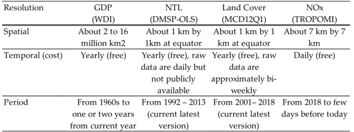
In this paper, we quantify the impact of various lockdown policy measures on economic activity. Since information on lockdown policy is available on a daily basis, we seek daily-level data on economic activity by country. Table 1 provides a comparison of spatial, temporal (including cost), and period data across selected ground-based and remote sensing data sources that have been used in the economic literature. Although gross domestic product (GDP) figures from the World Development Indicators (WDI) provided by the World Bank are available for the longest period of time, the temporal frequency (resolution) is yearly. In spite of its daily and global coverage, the validity of NTL data, which are the most widely used remotely sensed proxy for GDP, is not necessarily high due to missing or unreliable values resulting from bad weather. NTL data are generally available on an annual or monthly basis. The same is true for land cover data.
=== Table 1 ===
Against this backdrop, this paper instead turns to NOx data that are collected by the TROPOMI. NOx are important trace gases in the Earth’s atmosphere that result from anthropogenic activities (e.g., fossil fuel combustion and biomass burning) and natural processes (e.g., microbiological processes in soils, wildfires, and lightning).3 Demals et al. (1997) estimated the natural sources of NOx to be less than 30% of total global NOx emissions in the 1990s. After reviewing several previous studies, Weng et al. (2020) concluded that natural NOx (e.g., those generated by lightning) account for 15% or less of total NOx emissions globally in recent years. Economic activity causes the emission of both NTL and NOx. The former is caused by electricity consumption, while the latter by fuel burning. Both measures could be considered good proxies of GDP or gross regional product (GRP).
The NOx data used in this paper are downloaded through the Google Earth Engine. The Google Earth Engine excludes data cells (defined at 7 km by 7 km) with a reliability lower than 75% when pulling data from the ESA and converting them into a rasterized data format. The daily NOx data for a country are the sum of all reliable cells within the geographical boundaries of that country.4 We set the resolution for our downloading process to 10 km by 10 km instead of the 7 km by 7 km raw data resolution to speed up the
3 For more details, see http://www.tropomi.eu/data-products/nitrogen-dioxide. 4 The daily figure for the U.S. does not include the state of Alaska.
5
computational processes for nearly the entire globe. As a consequence, the daily NOx for each country should be considered an index of physical NOx units, which is comparable between countries and over time.
We used the remotely sensed data on NOx rather than the ground station-based data used in Deb et al. (2020). The latter covered only 62 countries while our data are available for over 200 countries. Aggregating air pollution statistics from satellite data is generally considered a top-down approach as opposed to compiling data from ground-based monitoring stations, which is considered a bottom-up approach. The top-down approach is superior in terms of spatial and temporal coverage but can be less accurate regarding emitter location because air pollutants are not fixed in space. For instance, the top-down NOx for a region might be affected by wind, as parts of emitted NOx could be blown through the air to neighboring regions. Some studies have also found that rainfall reduces air pollutant levels by washing them to the ground.
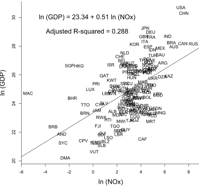
Figure 1 illustrates the relationship between our top-down NOx and WDI’s GDP in current United States (US) dollars in 2019. 2018 GDP was used for countries for which the latest figure was not yet available. Although variations exist, a high correlation between the two variables can be observed. On average, a 1% increase in NOx emissions increases GDP by 0.51%. In some countries/economies, GDP is relatively large, while NOx emissions are relatively small (e.g., Macau, Barbados, Bahrain, Singapore, and Hong Kong). On the other hand, the opposite relationship (i.e., a small GDP and large NOx) can be found in the Central African Republic, Greenland, and Mauritania. Since top-down NOx data are generated by the summation of remotely sensed NOx throughout space, they tend to be higher for countries with a large land area. Nevertheless, the population and therefore GDP are also generally higher for such countries. Thus, with proper controls, top-down NOx data are a good proxy for the level of the economy on the ground.
=== Figure 1 ===
The temporal frequency of remotely sensed NOx is outstanding. Figure 2 depicts daily NOx by selected country between January 1 and July 31, 2019 and the same period in 2020. At first glance, the daily data are not completely smooth due to many factors, including the effect of weather conditions and the omission of data based on reliability, as previously discussed. Nonetheless, NOx levels are generally smaller in 2020 than in 2019. The sum of NOx emissions for the aforementioned period in 2020 is about 15% to 31% smaller than during the same time period in 2019 for all selected countries, except for Brazil and South Africa. The reduction of NOx in Japan, China, India, and Thailand is concentrated between the 100th and 150th days of the year, i.e., April and May. This coincides with intensified lockdown measures in these countries. It is not entirely clear why the reduction in Brazil and South Africa is so small compared to the other countries, although the former is known
6
to have a leadership that is very skeptical of the need for lockdown policy. Even so, a sharp decrease in NOx can be observed between the 100th and 150th days in both countries. We consider this as evidence demonstrating that NOx emissions not only reflect the level of economic activity on the ground but do so in a way that reveals daily variations.
=== Figure 2 ===
3.
Empirical Framework
This section presents the empirical framework used to investigate the impact of lockdown policy on NOx emissions. As major lockdown measures, we focus on the workplace-closing policy and the stay-at-home policy. As mentioned in the introductory section, the major sources of NOx include fuel burning in factories, thermal power plants, residential activity, and the emissions of gas by passenger cars, buses, and trucks. In residential areas, the use of natural gas boilers for cooking and fireplaces for heating are typical sources of NOx emissions. The use of electricity at home might also result in the active operation of thermal power plants and therefore higher NOx emissions. When the workplace-closing policy becomes effective, the closure of factories and reduction in commuting by cars will decrease NOx emissions. On the other hand, working at home instead of at factories or in offices might increase emissions due to the additional time spent in residential areas.5 Similar effects can be expected for the stay-at-home policy. NOx emissions increase due to the longer time spent in residential areas, while it decreases due to decreased use of cars for shopping. Therefore, there will be both increasing and decreasing forces at work related to the implementation of the workplace-closing and stay-at-home policies.
An empirical analysis is conducted on the country-daily level. We examine 173 countries for which all of the variables used in our empirical analysis were available, listed in Appendix A. The study period extends from January 1 to July 31, 2020. Following Deb et al. (2020), we specify the estimation model as follows.
ln𝑁𝑁𝑁𝑁𝑁𝑁𝑖𝑖𝑖𝑖𝑖𝑖 =𝛼𝛼1×𝑊𝑊𝑊𝑊𝑊𝑊𝑊𝑊𝑊𝑊𝑊𝑊𝑊𝑊𝑊𝑊𝑊𝑊𝑖𝑖𝑖𝑖𝑖𝑖+𝛼𝛼2×𝑆𝑆𝑆𝑆𝑊𝑊𝑆𝑆𝑖𝑖𝑖𝑖𝑖𝑖 +𝐙𝐙′𝛃𝛃+𝛿𝛿𝑖𝑖+𝛿𝛿𝑖𝑖𝑖𝑖+𝜖𝜖𝑖𝑖𝑖𝑖𝑖𝑖 (1)
where 𝑁𝑁𝑁𝑁𝑁𝑁𝑖𝑖𝑖𝑖𝑖𝑖 is NOx emissions in country i on date d in month m in 2020. 𝑊𝑊𝑊𝑊𝑊𝑊𝑊𝑊𝑊𝑊𝑊𝑊𝑊𝑊𝑊𝑊𝑊𝑊𝑖𝑖𝑖𝑖𝑖𝑖
takes a value of one if country i imposes the workplace-closing policy on date d in month m.
5 For example, the following articles claim that staying at home could be worse for energy consumption:
https://www.swissinfo.ch/eng/coronavirus-and-the-climate_can-covid-19-help-the-environment-/45670634;
https://www.stir.ac.uk/news/2020/09/lockdown-did-not-reduce-most-harmful-type-of-air-pollution-in-scotland/.
7
Similarly, 𝑆𝑆𝑆𝑆𝑊𝑊𝑆𝑆𝑖𝑖𝑖𝑖𝑖𝑖 is a dummy variable for the stay-at-home policy. As mentioned above, there are both positive and negative effects on NOx emissions. The coefficients for the two lockdown policy variables will indicate their net effect. 𝜖𝜖𝑖𝑖𝑖𝑖𝑖𝑖 is a disturbance term. We estimate this equation using the ordinary least squares (OLS) method.
A vector of Z includes various control variables. First, to reduce the risk of omitted variable bias, we control for the log of COVID-19 cases (Deb et al., 2020). A growing number of cases encourages governments to introduce lockdown measures. At the same time, people will hesitate to leave home and thereby decrease NOx emissions. For the same reason, we also introduce the log of COVID-19 deaths. This variable controls for NOx emissions due to cremation. Second, as mentioned in Section 2, previous studies have demonstrated the effect of climate conditions on NOx emissions. To control for variations in NOx due to those conditions, we introduce temperature, the amount of rainfall, and the amount of wind. In addition to these variables, we also control for two kinds of fixed effects. 𝛿𝛿𝑖𝑖 is country fixed effects, which control for country-specific elements that affect NOx emissions, including country size, environmental technology, and environmental regulations. 𝛿𝛿𝑖𝑖𝑖𝑖 is month-date fixed effects, which control for global shocks on NOx emissions.
Our data sources are as follows. The data source for NOx emissions is the same as that introduced in Section 2, which is data remotely sensed by TROPOMI. Data on the number of COVID-19 cases were obtained from the European Centre for Disease Prevention and Control.6 These data have been collected on a daily basis from health authorities worldwide. We obtained data on weather conditions from the Global Summary of the Day, from the US National Centers for Environmental Information, from which the latest data are normally available within one to two days for over 9,000 stations worldwide. Mean temperature, mean precipitation, and mean wind speed were used as control variables in our empirical analysis.
The data on the 𝑊𝑊𝑊𝑊𝑊𝑊𝑊𝑊𝑊𝑊𝑊𝑊𝑊𝑊𝑊𝑊𝑊𝑊𝑖𝑖𝑖𝑖𝑖𝑖 and 𝑆𝑆𝑆𝑆𝑊𝑊𝑆𝑆𝑖𝑖𝑖𝑖𝑖𝑖 variables were obtained from the Oxford COVID-19 Government Response Tracker (OxCGRT) (Hale et al., 2020). The OxCGRT systematically collects information on several government policy responses to the pandemic for over 160 countries. As a measure of 𝑊𝑊𝑊𝑊𝑊𝑊𝑊𝑊𝑊𝑊𝑊𝑊𝑊𝑊𝑊𝑊𝑊𝑊𝑖𝑖𝑖𝑖𝑖𝑖, we use “C2 Workplace closing,” which includes “1 - recommend closing (or recommend work from home),” “2 - require closing (or work from home) for some sectors or categories of workers,” and “3 - require closing (or work from home) for all-but-essential workplaces (e.g., grocery stores, and doctors).” The measure of 𝑆𝑆𝑆𝑆𝑊𝑊𝑆𝑆𝑖𝑖𝑖𝑖𝑖𝑖 is constructed using “C6 Stay-at-home requirements,” which includes “1 - recommend not leaving house,” “2 - require not leaving house with exceptions for daily exercise, grocery shopping, and 'essential' trips,” and “3 - require not leaving house with minimal exceptions (e.g., allowed to leave once a week, only one person can leave at a time, etc.).” We call the policy with a degree of 1 a “recommend-base policy” while that with a degree of 2 or 3 is called a “require-“recommend-base policy.” Obviously,
8
the latter is more restrictive than the former. In the baseline analysis, we use lockdown dummy variables that take a value of one if only the require-base policy is effective.
4.
Empirical Results
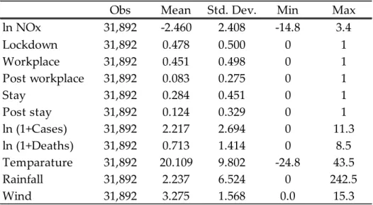
This section reports the estimation results. The basic statistics are shown in Table 2. After reporting our baseline results, we show the results of some extended models.
=== Table 2 ===
4.1. Baseline Results
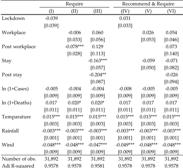
The baseline results are shown in Column (I) in Table 3. We cluster the standard errors by country. In this equation, we do not differentiate between stay-at-home and workplace-closing policies and examine the Lockdown dummy, which takes a value of one if either policy variable takes the value one. The coefficient for Lockdown is estimated to be negative but insignificant. Thus, on average, it does not have a significant effect on NOx emissions. Among the control variables, the number of COVID-19 cases and deaths do not have significant coefficients, while the coefficients for weather-related variables are significantly estimated. NOx emissions are larger when the temperature is higher, the amount of rainfall is lower, and the wind is weaker. In Column (II), we differentiate between the two policies. While the coefficient for the workplace-closing policy is estimated to be insignificant, the stay-at-home policy dummy has a significantly negative coefficient. The latter result indicates that the introduction of the stay-at-home policy significantly reduces NOx emissions. Another noteworthy difference lies in the coefficient for the number of deaths, which is estimated to be significantly positive.
=== Table 3 ===
In Column (III), we divide the no-lockdown policy period between the pre- and post-policy periods by introducing the Post workplace and Post stay dummies. To construct these dummy variables, we first identify the final date when each lockdown policy was effective, i.e., when Workplace and Stay take a value of one. Then, the Post workplace and Post stay
dummies take a value of one if the study date occurs after that final date. The results for the workplace-closing policy are unchanged. During both the lockdown period and the post-lockdown period, the workplace-closing policy does not have a significant effect on NOx emissions. In the case of the stay-at-home policy, on the other hand, both the lockdown and post-lockdown dummies have significantly negative coefficients. These results indicate that
9
NOx emissions significantly decrease not only during the stay-at-home policy period but also after it. It might be a surprising result that the latter period has a larger absolute coefficient, suggesting that the decrease in NOx emissions is more substantial after than during the stay-at-home policy.
In Columns (IV)-(VI), we replace the lockdown dummy variables with those based on the existence of any degree of policy (i.e., either recommend-base or require-base). All lockdown-related variables have insignificant coefficients. If we expand the definition of lockdown policy to the recommend-base policy, we do not find any significant effect on NOx emissions. This result implies that NOx emissions do not substantially decrease during the recommend-base policy period. Thus, if we exclude this period from the base period in the dummy variables, NOx emissions during the lockdown policy period are not significantly different from those during the base period. The results for the other variables are qualitatively unchanged.
4.2. Extension
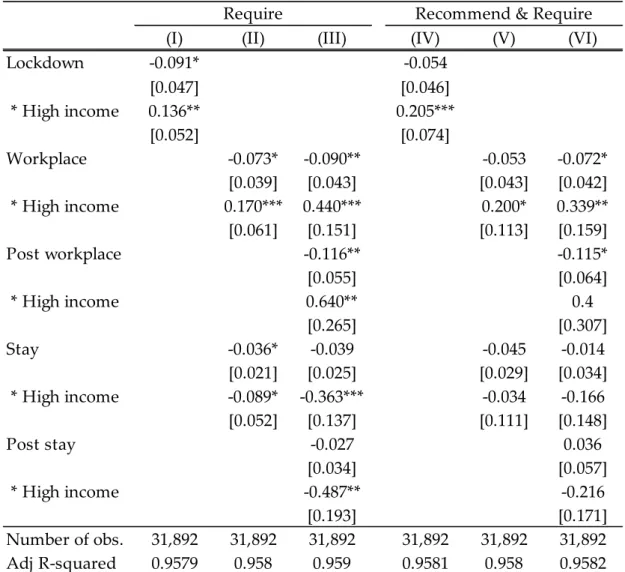
Next, we examine differences in the effects between high- and low-income countries by introducing interaction terms with a dummy variable that takes a value of one if a country is classified as high-income by the World Bank income classification. The results are shown in Table 4. The results for the control variables are omitted to save space. Column (I) indicates that lockdown policy significantly reduces NOx emissions in low-income countries but does not in high-income countries. This difference in the effect between high- and low-income countries yields insignificant results in Column (I) in Table 3. Such results can be found in the case of the workplace-closing policy, as shown in Column (II). The workplace-closing policy significantly decreases NOx emissions in low-income countries but does not in high-income countries. Rather, their amount increases during the workplace-closing policy. We do not find a significant difference between the two groups of countries in the effect of the stay-at-home policy.
=== Table 4 ===
In Column (III), which shows the results for the equation with the Post workplace
dummy, the Post stay dummy, and their interaction terms, we encounter more interesting results. The workplace-closing policy significantly decreases NOx emissions in low-income countries during the policy and post-policy periods. The magnitude of the decrease is slightly larger during the post-policy period than during the policy period. However, it does not decrease in high-income countries during both periods. Rather, in high-income countries, NOx emissions increase during both periods, especially the post-policy period. Conversely, the stay-at-home policy reduces NOx emissions in high-income countries. Such
10
a reduction can be found during both the policy and post-policy periods. In Columns (IV)-(VI), we use the dummy variables based on any degree of policy. Compared with the results in Columns (I)-(III), some coefficients turned out to be insignificant.
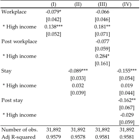
Before moving to the next analysis, it is worth noting the possibility of multicollinearity bias. During the lockdown period, the workplace-closing policy and stay-at-home policy tend to overlap. Although we can identify their effects separately because their starting and ending dates usually differ, our estimates might suffer from multicollinearity bias. To check this possibility, in Table B1 in Appendix B, we estimate our models by separately introducing these two policies. The difference lies in the results for the stay-at-home policy, which has a significantly negative effect on NOx emissions in both high- and low-income countries during both the policy and post-policy periods. Thus, it is safe not to emphasize the difference between high- and low-income countries in the effect of the stay-at-home policy. On the other hand, we still find a difference in the effect of the workplace-closing policy similar to that in Table 4.
Table 5 reports the results of the equations that add the interaction terms with regional dummy variables. In the analyses below, we focus on the dummy variables based on the require-base policy. With the regional classification in OxCGRT, we classify the world into seven regions. The base region is East Asia and the Pacific. Thus, the results in the other regions show additional effects to those in this base region. Models (I) and (II) indicate that the workplace-closing policy reduces NOx emissions but does not in Europe & Central Asia and North America. These results are consistent with those in Column (II) in Table 3 because non-decreasing regions consist mostly of high-income countries.
=== Table 5 ===
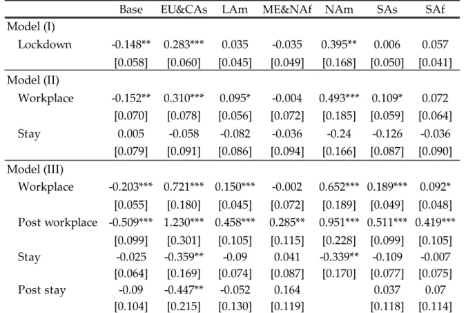
Model (III) exhibits interesting results. Compared with NOx emissions before the workplace-closing policy, during the workplace-closing policy, their amount decreases significantly worldwide, except for Europe & Central Asia and North America. The negative effect of the workplace-closing policy is small or almost zero in Latin America and South Asia. After lifting the workplace-closing policy, NOx emissions decrease considerably only in East Asia and the Pacific. The absolute magnitude of the decrease in this region is larger during the post-policy period than during the policy period. In other regions, their amount returns to the pre-policy level. In Europe & Central Asia and North America, emissions increase. The absolute magnitude of the increase is larger during the post-policy period than during the policy period. On the other hand, the stay-at-home policy decreases NOx emissions only in Europe & Central Asia and North America. In these regions, emissions decline both during the and after the policy period.7
7 These results were unchanged even after we introduced region-month fixed effects to control for
11
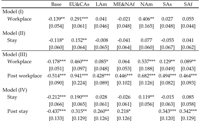
We again check if our estimates suffer from multicollinearity bias. In Table B2 in Appendix B, we estimate our models by separately introducing these two policies. Like the previous case, the difference lies in the results for the stay-at-home policy. When we introduce the two policy variables simultaneously (i.e., Table 5), we find a larger negative effect of the stay-at-home policy in Europe & Central Asia and North America than in the base region, i.e., East Asia and the Pacific. However, when introducing those policy variables separately, the negative effects become larger in East Asia and the Pacific than in Europe & Central Asia and North America. Thus, it is again safe not to emphasize the difference between regions in the effect of the stay-at-home policy. On the other hand, we still find a difference in the effect of the workplace-closing policy similar to those in Table 5.
4.3. Other Lockdown Policies
Lastly, we examine the effects of other types of lockdown policies. Specifically, we introduce five additional types, including School (closings of schools and universities),
Meeting (limits on private gatherings), Transport services (closing of public transportation),
Domestic travel (restrictions on internal movement between cities and regions), and
International travel (restrictions on international travel against foreign travelers). Again, these
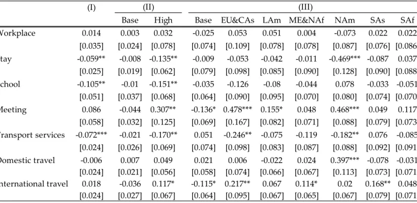
dummy variables take the value of one if the require-base restriction is imposed. The results are shown in Column (I) in Table 6. In addition to the stay-at-home policy, the school-closing policy and the public transportation-closing policy have significantly negative effects on NOx emissions. The school-closing policy has the largest quantitative effect, on average. This result might indicate that activity by teenagers accounts for a significant fraction of national NOx emissions. In addition, since public transportation is one of the most important sources of NOx emissions, it is natural to see a negative effect from its restriction.
=== Table 6 ===
In Column (II), we differentiate between countries according to their income level. The baseline category is low-income countries. Thus, the “High” column indicates the additional effect in high-income countries. The “Base” column suggests no significant effect of lockdown policy in low-income countries. However, a significant effect in high-income countries can be found with the school-closing policy, public transportation-closing policy, private meeting-restriction policy, and international travel restriction policy. The former two policies reduce NOx emissions, while the latter two increase them. The significant result for the school-closing policy for high-income countries might be related to the relatively high gross enrollment rates in high-income countries. The increase in the latter two policies is a bit puzzling. Although the international travel restriction policy bans the entry of foreigners, it often requires domestic residents to quarantine for 14 days when they return
12
from travel abroad. Therefore, to avoid this quarantine, domestic residents might switch to domestic travel, resulting in an increase of NOx emissions.
Column (III) reports the results according to region. Again, the base region is East Asia and the Pacific. Most of the coefficients are insignificantly estimated. Significant results can be found in Europe, Central Asia, and North America. In these regions, the public transportation-closing policy decreases NOx emissions, while they increase when the private meeting-restriction policy is in effect. In addition, the stay-at-home policy reduces NOx emissions in North America, while they increase when the international trade-restriction policy is in effect. Overall, we can observe many variations in the effect of lockdown policy according to region.
5.
Concluding Remarks
In this study, we empirically investigated how much human economic and social activity decreased as a result of implementing lockdown policy during the COVID-19 pandemic using daily data on NOx emissions from 173 countries between January 1 and July 31, 2020. We encountered many differences in the effects of the workplace-closing and stay-at-home policies on NOx emissions according to various dimensions. The workplace-closing policy significantly decreases NOx emissions in low-income countries (i.e., East Asia and the Pacific) during the policy and post-policy periods. However, in high-income countries (i.e., Europe & Central Asia and North America) NOx emissions increase during both periods. It is also found that the absolute impact of the workplace-closing policy is larger during the post-policy period than during the policy period. While the stay-at-home policy reduces NOx emissions, we do not discover robust differences in its effect between regions.
The decrease in NOx emissions in low-income countries (i.e., East Asia and the Pacific) caused by the workplace-closing policy implies that its negative effect is stronger than its positive effect. Since production technology in these countries is less eco-friendly than in developed countries, stopping such a production facility decreases NOx emissions considerably. In addition, East Asian countries include cities known to have terrible traffic congestion (e.g., Manila, Jakarta, and Bangkok). Since one reason for such congestion is that people use cars to commute to work, the decrease in the use of cars caused by the workplace-closing policy dramatically reduces NOx emissions. As a result of these negative effects, net NOx emissions decrease in these countries or regions.
Conversely, in high-income countries (i.e., Europe & Central Asia and North America) the net effect of the workplace-closing policy is positive. The remote work or work-from-home policy consumes a larger amount of energy on a national level than office work. Indeed, the raw data for Europe indicate that the sharp decline in high-level emissions in
13
urban areas was offset and slightly overwhelmed by the increase in low-level emissions in non-urban areas. Such an increase in energy consumption due to everyone working from home might contribute to greatly increasing NOx emissions in those regions. By contrast, due to the use of relatively eco-friendly manufacturing facilities, the negative effect of factory closures was small. As a result, net NOx emissions increase in these countries or regions.
Lastly, the larger magnitude of the absolute impact during the post-policy period indicates the following two human behaviors. One is that people might not fully react to lockdown policy at the beginning of the policy period. Since most people have never previously experienced this level of lockdown, they did not know how to behave and how much to comply with such restrictions. Therefore, people might have gradually stopped their social activity, especially at the beginning of the policy period. The other behavior is that people might not have returned to normal practices even after lockdown policy was lifted. Since the discontinuation of the policy does not mean the end of the COVID-19 pandemic, people maintained infection control measures (e.g., social distancing, working from home). These two behaviors cause the impact on NOx emissions to be larger in the post-policy period than during the policy period.
14
References
Adams, Matthew, 2020, Air pollution in Ontario, Canada during the COVID-19 State of Emergency, Science of The Total Environment, 742. 140516.
Almond, Douglas, Xinming Du, and Shuang Zhang, 2020, Ambiguous Pollution Response to Covid-19 in China, NBER Working Papers 27086, National Bureau of Economic Research, Inc.
Askitas, Nikos, Konstantinos Tatsiramos, and Bertrand Verheyden, 2020, Lockdown Strategies, Mobility Patterns and Covid-19, Covid Economics, 23: 263-302.
Baldasano, José M., 2020, COVID-19 Lockdown Effects on Air Quality by NO2 in the Cities of Barcelona and Madrid (Spain), Science of the Total Environment, 741: 140353.
Chang, Hung-Hao, Chad Meyerhoefer, and Feng-An Yang, 2020, COVID-19 Prevention and Air Pollution in the Absence of a Lockdown, NBER Working Papers 27604, National Bureau of Economic Research, Inc.
Chen, Kai, Meng Wang, Conghong Huang, Patrick L Kinney, and Paul T Anastas, 2020, Air pollution reduction and mortality benefit during the COVID-19 outbreak in China,
The Lancet Planetary Health, 4(6): e210-e212.
Chen, Xi and William D. Nordhaus, 2011, Using Luminosity Data as a Proxy for Economic Statistics, Proceedings of the National Academy of Sciences, 108(21): 8589-8594.
Cicala, Steve, Stephen P. Holland, Erin T. Mansur, Nicholas Z. Muller, and Andrew J. Yates, 2020, Expected Health Effects of Reduced Air Pollution from COVID-19 Social Distancing, NBER Working Papers 27135, National Bureau of Economic Research, Inc. Coibion, Olivier, Yuriy Gorodnichenko, and Michael Weber, 2020, Lockdowns,
Macroeconomic Expectations, and Consumer Spending, Covid Economics, 20: 1-15. Cole, Matthew A, Robert J R Elliott, and Bowen Liu, 2020, The Impact of the Wuhan
Covid-19 Lockdown on Air Pollution and Health: A Machine Learning and Augmented Synthetic Control Approach, Discussion Papers 20-09, Department of Economics, University of Birmingham.
Collivignarelli, Maria Cristina, Alessandro Abbà, Giorgio Bertanza, Roberta Pedrazzani, Paola Ricciardi, and Marco Carnevale Miino, 2020, Lockdown for CoViD-2019 in Milan: What are the Effects on Air Quality?, Science of the Total Environment, 732: 139280. Conyon, Martin J., Lerong He, and Steen Thomsen, 2020, Lockdowns and COVID-19
Deaths in Scandinavia, Covid Economics, 26: 17-42.
Dang, Hai-Anh H. and Trong-Anh Trinh, 2020, Does the COVID-19 Pandemic Improve Global Air Quality? New Cross-National Evidence on Its Unintended Consequences, IZA DP No. 13480.
15
Effects of Covid-19 Containment Measures, Covid Economics, 24: 32-75.
Donaldson, Dave and Adam Storeygard, 2016, The View from Above: Applications of Satellite Data in Economics, Journal of Economic Perspectives, 30(4): 171–198.
Eaton, Jonathan, Samuel Kortum, Brent Neiman, and John Romalis, 2016, Trade and the Global Recession, American Economic Review, 106(11): 3401-3438.
Fan, Cheng, Ying Li, Jie Guang, Zhengqiang Li, Abdelrazek Elnashar, Mona Allam, and Gerrit de Leeuw, 2020, The Impact of the Control Measures during the COVID-19 Outbreak on Air Pollution in China, Remote Sensing, 12(10): 1613.
Ghosh, Saibal, 2020, Lockdown, Pandemics and Quarantine: Assessing the Indian Evidence,
Covid Economics, 37: 73-99.
Gonzalez-Eiras, Martín and Dirk Niepelt, 2020, On the Optimal “Lockdown” during an Epidemic, Covid Economics, 7: 68-87.
Hale, Thomas, Sam Webster, Anna Petherick, Toby Phillips, and Beatriz Kira, 2020, Oxford
COVID-19 Government Response Tracker, Blavatnik School of Government.
Hayakawa, Kazunobu and Hiroshi Mukunoki, 2020, Impacts of Lockdown Policies on International Trade, IDE Discussion Paper 798.
Henderson, Vernon J., Adam Storeygard, and David N. Weil, 2012, Measuring Economic Growth from Outer Space, American economic review, 102(2): 994-1028.
Inoue, Hiroyasu and Yasuyuki Todo, 2020, The Propagation of the Economic Impact through Supply Chains: The Case of a Mega-city Lockdown to Contain the Spread of Covid-19, Covid Economics, 2: 43-59.
Jean, Neal, Marshall Burke, Michael Xie, Matthew W. Davis, David B. Lobell, and Stefano Ermon, 2016, Combining Satellite Imagery and Machine Learning to Predict Poverty,
Science, 353(6301): 790-794.
Keola, Souknilanh, Magnus Andersson, and Ola Hall, 2015, Monitoring Economic Development from Space: Using Nighttime Light and Land Cover Data to Measure Economic Growth, World Development, 66: 322-334.
Kong, Edward and Daniel Prinz, 2020, The Impact of Shutdown Policies on Unemployment during a Pandemic, Covid Economics, 17: 24-72.
Kumar, Sandeep and Pranab K. Muhuri, 2019, A Novel GDP Prediction Technique Based on Transfer Learning Using CO2 Emission Dataset, Applied Energy, 253: 113476.
Kwak, Ha-Young, Joonho Ko, Seungho Lee, Chang-Hyeon Joh, 2017, Identifying the Correlation between Rainfall, Traffic Flow Performance and Air Pollution Concentration in Seoul Using a Path Analysis, Transportation Research Procedia, 25: 3552-3563.
Leibovici, Fernando and Ana Maria Santacreu, 2020, International Trade of Essential Goods during a Pandemic, Covid Economics, 21: 59-99.
Guo, Ling-Chuan, Yonghui Zhang, Hualiang Lin, Weilin Zeng,Tao Liu, Jianpeng Xiao,
16
Rainfall on Atmospheric Particulate Pollution in Two Chinese Cities, Environmental
Pollution, 215: 195-202.
Isphording, Ingo E. and Nico Pestel, 2020, Pandemic Meets Pollution: Poor Air Quality Increases Deaths by COVID-19, IZA DP No. 13418.
Mahato, Susanta, Swades Pal, and Krishna Gopal Ghosh, 2020, Effect of Lockdown amid COVID-19 Pandemic on Air Quality of the Megacity Delhi, India, Science of the Total
Environment, 730: 139086.
Menut, Laurent, Bertrand Bessagnet, Guillaume Siour, Sylvain Mailler, Romain Pennel, and Arineh Cholakian, 2020, Impact of lockdown measures to combat Covid-19 on air quality over western Europe, Science of the Total Environment, 741: 140426.
Pei, Zhipeng, Ge Han, Xin Ma, Hang Su, and Wei Gong, 2020, Response of major air pollutants to COVID-19 lockdowns in China, Science of the Total Environment, 743: 140879.
Pichler, Anton, Marco Pangallo, R. Maria del Rio-Chanona, François Lafond, and J. Doyne Farmer, 2020, Production Networks and Epidemic Spreading: How to Restart the UK Economy?, Covid Economics, 23: 79-151.
Shi, Xiaoqin and Guy P. Brasseur, 2020, The Response in Air Quality to the Reduction of Chinese Economic Activities during the COVID-19 Outbreak, Geophysical Research
Letters, 47: e2020GL088070.
Ullah, Akbar and Olubunmi Agift Ajala, 2020, Do Lockdown and Testing Help in Curbing Covid-19 Transmission?, Covid Economics, 13: 138-156.
Wang, Yichen, Yuan Yuan, Qiyuan Wang, Chen Guang Liu, Qiang Zhi, and Junji Cao, 2020, Changes in Air Quality Related to the Control of Coronavirus in China: Implications for Traffic and Industrial Emissions, Science of the Total Environment, 73: 139133.
Zangari, Shelby, Dustin T. Hill, Amanda T. Charette, and Jaime E. Mirowsky, 2020, Air Quality Changes in New York City during the COVID-19 Pandemic, Science of The Total
17
Table 1. Comparison of Selected Ground-based and Remote-sensing Data
Resolution GDP NTL Land Cover NOx
(WDI) (DMSP-OLS) (MCD12Q1) (TROPOMI)
Spatial About 2 to 16
million km2 1km at equatorAbout 1 km by About 1 km by 1km at equator About 7 km by 7km Temporal (cost) Yearly (free) Yearly (free), raw
data are daily but not publicly
available
Yearly (free), raw data are approximately
bi-weekly
Daily (free)
Period From 1960s to
one or two years from current year
From 1992 – 2013 (current latest version) From 2001– 2018 (current latest version) From 2018 to few days before today Notes: WDI = World Development Indicators (The World Bank); DMSP-OLS = Defense Meteorological Satellite – Operational Linescan Systems (US Department of Defense); MODIS = Moderate Resolution Imaging Spectroradiometer (National Aeronautics and Space Administration, NASA); and TROPOMI = TROPOspheric Monitoring Instrument (European Space Agency, ESA).
18 Table 2. Basic Statistics
Obs Mean Std. Dev. Min Max
ln NOx 31,892 -2.460 2.408 -14.8 3.4 Lockdown 31,892 0.478 0.500 0 1 Workplace 31,892 0.451 0.498 0 1 Post workplace 31,892 0.083 0.275 0 1 Stay 31,892 0.284 0.451 0 1 Post stay 31,892 0.124 0.329 0 1 ln (1+Cases) 31,892 2.217 2.694 0 11.3 ln (1+Deaths) 31,892 0.713 1.414 0 8.5 Temparature 31,892 20.109 9.802 -24.8 43.5 Rainfall 31,892 2.237 6.524 0 242.5 Wind 31,892 3.275 1.568 0.0 15.3
19 Table 3. Estimation Results
(I) (II) (III) (IV) (V) (VI)
Lockdown -0.039 0.031 [0.039] [0.033] Workplace -0.006 0.060 0.026 0.054 [0.033] [0.056] [0.053] [0.046] Post workplace -0.078*** 0.129 0.073 [0.028] [0.113] [0.140] Stay -0.163*** -0.059 -0.071 [0.057] [0.050] [0.082] Post stay -0.204** -0.026 [0.087] [0.094] ln (1+Cases) -0.005 -0.004 -0.004 -0.008 -0.005 -0.005 [0.009] [0.009] [0.009] [0.009] [0.009] [0.009] ln (1+Deaths) 0.017 0.020* 0.020* 0.017 0.017 0.017 [0.011] [0.011] [0.011] [0.011] [0.011] [0.011] Temparature 0.015*** 0.015*** 0.015*** 0.015*** 0.015*** 0.015*** [0.003] [0.003] [0.003] [0.003] [0.003] [0.003] Rainfall -0.003*** -0.003*** -0.003*** -0.003*** -0.003*** -0.003*** [0.001] [0.001] [0.001] [0.001] [0.001] [0.001] Wind -0.048*** -0.048*** -0.047*** -0.049*** -0.048*** -0.048*** [0.009] [0.009] [0.009] [0.009] [0.009] [0.009] Number of obs. 31,892 31,892 31,892 31,892 31,892 31,892 Adj R-squared 0.9578 0.9578 0.9581 0.9578 0.9578 0.9578
Require Recommend & Require
Notes: This table reports the estimation results obtained using the ordinary least squares (OLS) method. The dependent variable is the log of NOx emissions. ***, **, and * indicate, respectively, the 1%, 5%, and 10% levels of statistical significance. The standard errors reported in parentheses are clustered by country. In all specifications, we control for country fixed effects and date fixed effects. In the column “Recommend & Require,” the lockdown dummy variables take a value of one if at least the recommend-base policy becomes effective. In the column “Require,” the lockdown dummy variables take a value of one if only the require-base policy becomes effective.
20
Table 4. High-income Countries versus Low-income Countries
(I) (II) (III) (IV) (V) (VI)
Lockdown -0.091* -0.054 [0.047] [0.046] * High income 0.136** 0.205*** [0.052] [0.074] Workplace -0.073* -0.090** -0.053 -0.072* [0.039] [0.043] [0.043] [0.042] * High income 0.170*** 0.440*** 0.200* 0.339** [0.061] [0.151] [0.113] [0.159] Post workplace -0.116** -0.115* [0.055] [0.064] * High income 0.640** 0.4 [0.265] [0.307] Stay -0.036* -0.039 -0.045 -0.014 [0.021] [0.025] [0.029] [0.034] * High income -0.089* -0.363*** -0.034 -0.166 [0.052] [0.137] [0.111] [0.148] Post stay -0.027 0.036 [0.034] [0.057] * High income -0.487** -0.216 [0.193] [0.171] Number of obs. 31,892 31,892 31,892 31,892 31,892 31,892 Adj R-squared 0.9579 0.958 0.959 0.9581 0.958 0.9582
Require Recommend & Require
Notes: This table reports the estimation results obtained using the ordinary least squares (OLS) method. The dependent variable is the log of NOx emissions. ***, **, and * indicate, respectively, the 1%, 5%, and 10% levels of statistical significance. The standard errors reported in parentheses are clustered by country. In all specifications, we control for country fixed effects and date fixed effects. We do not report the results for control variables (e.g., weather-related variables). In the column “Recommend & Require,” the lockdown dummy variables take a value of one if at least the recommend-base policy becomes effective. In the column “Require,” the lockdown dummy variables take a value of one only if the require-base policy becomes effective.
21 Table 5. Estimation Results by Region
Base EU&CAs LAm ME&NAf NAm SAs SAf Model (I) Lockdown -0.148** 0.283*** 0.035 -0.035 0.395** 0.006 0.057 [0.058] [0.060] [0.045] [0.049] [0.168] [0.050] [0.041] Model (II) Workplace -0.152** 0.310*** 0.095* -0.004 0.493*** 0.109* 0.072 [0.070] [0.078] [0.056] [0.072] [0.185] [0.059] [0.064] Stay 0.005 -0.058 -0.082 -0.036 -0.24 -0.126 -0.036 [0.079] [0.091] [0.086] [0.094] [0.166] [0.087] [0.090] Model (III) Workplace -0.203*** 0.721*** 0.150*** -0.002 0.652*** 0.189*** 0.092* [0.055] [0.180] [0.045] [0.072] [0.189] [0.049] [0.048] Post workplace -0.509*** 1.230*** 0.458*** 0.285** 0.951*** 0.511*** 0.419*** [0.099] [0.301] [0.105] [0.115] [0.228] [0.099] [0.105] Stay -0.025 -0.359** -0.09 0.041 -0.339** -0.109 -0.007 [0.064] [0.169] [0.074] [0.087] [0.170] [0.077] [0.075] Post stay -0.09 -0.447** -0.052 0.164 0.037 0.07 [0.104] [0.215] [0.130] [0.119] [0.118] [0.114] Notes: This table reports the estimation results obtained using the ordinary least squares (OLS) method. The dependent variable is the log of NOx emissions. ***, **, and * indicate, respectively, the 1%, 5%, and 10% levels of statistical significance. The standard errors reported in parentheses are clustered by country. In all specifications, we control for country fixed effects and date fixed effects. We do not report the results for control variables (e.g., weather-related variables). In this table, we use the lockdown dummy variables based on “Require,” which take a value of one if only the require-base policy becomes effective. For the interaction terms of the lockdown variables with regional dummy variables, the base region is East Asia and the Pacific. “EU&CAs,” “LAm,” “ME&NAf,” “NAm,” “SAs,” and “SAf,” respectively, represent Europe and Central Asia, Latin America, Middle East and North Africa, North America, South Asia, and South Africa.
22 Table 6. Estimation Results by Lockdown Policy
(I)
Base High Base EU&CAs LAm ME&NAf NAm SAs SAf Workplace 0.014 0.003 0.032 -0.025 0.053 0.051 0.004 -0.073 0.022 0.022 [0.035] [0.024] [0.078] [0.074] [0.109] [0.078] [0.078] [0.087] [0.076] [0.086] Stay -0.059** -0.008 -0.135** -0.009 -0.053 -0.042 -0.011 -0.469*** -0.087 0.037 [0.025] [0.019] [0.062] [0.079] [0.098] [0.085] [0.090] [0.128] [0.090] [0.088] School -0.105** -0.01 -0.151** -0.035 -0.126 -0.08 -0.044 0.078 -0.033 -0.051 [0.051] [0.037] [0.068] [0.064] [0.090] [0.095] [0.070] [0.080] [0.074] [0.070] Meeting 0.086 -0.044 0.307** -0.136* 0.478*** 0.155* 0.048 0.468*** 0.049 0.117 [0.058] [0.032] [0.125] [0.069] [0.167] [0.082] [0.071] [0.088] [0.079] [0.073] Transport services -0.072*** -0.021 -0.170** 0.051 -0.246** -0.075 -0.119 -0.182** 0.076 -0.085 [0.024] [0.026] [0.069] [0.074] [0.098] [0.083] [0.087] [0.088] [0.092] [0.091] Domestic travel -0.006 0.007 0.049 0.021 0.006 -0.022 0.024 0.397*** -0.078 -0.031 [0.024] [0.021] [0.056] [0.058] [0.074] [0.066] [0.067] [0.113] [0.073] [0.071] International travel 0.018 -0.036 0.117* -0.115* 0.217** 0.067 0.114* 0.02 0.168** 0.048 [0.024] [0.027] [0.067] [0.064] [0.095] [0.067] [0.065] [0.067] [0.079] [0.071] (II) (III)
Notes: This table reports the estimation results obtained using the ordinary least squares (OLS) method. The dependent variable is the log of NOx emissions. ***, **, and * indicate, respectively, the 1%, 5%, and 10% levels of statistical significance. The standard errors reported in parentheses are clustered by country. In all specifications, we control for country fixed effects and date fixed effects. We do not report the results for control variables (e.g., weather-related variables). In this table, we use the lockdown dummy variables based on “Require,” which take a value of one if only the require-base policy becomes effective. For the interaction terms of the lockdown variables with regional dummy variables, the base region is East Asia and the Pacific. “EU&CAs,” “LAm,” “ME&NAf,” “NAm,” “SAs,” and “SAf,” respectively, represent Europe and Central Asia, Latin America, Middle East and North Africa, North America, South Asia, and South Africa.
23 Figure 1. Correlation between NOx and GDP in 2019
Source: Computed by the authors based on TROPMI and WDI. Note: The figure for US excludes the state of Alaska.
24
Figure 2. Daily NOx by Selected Country (January 1–July 31st, 2019 and 2020)
Source: Computed by the authors based on TROPMI and WDI. Figures in brackets represent the change in total NOx between January 1-July 29, 2020 and January 1-July 29, 2019.
25
Appendix A. Study Countries (173)
East Asia & PacificAUS*, BRN*, CHN, FJI, GUM*, HKG*, IDN, JPN*, KHM, KOR*, LAO, MAC*, MMR, MNG, MYS, NZL*, PHL, PNG, SGP*, SLB, THA, TLS, TWN*, VNM, VUT
Europe & Central Asia
ALB, AND*, AUT*, AZE, BEL*, BGR, BIH, BLR, CHE*, CYP*, CZE*, DEU*, DNK*, ESP*, EST*, FIN*, FRA*, GBR*, GEO, GIB*, GRC*, GRL*, HRV*, HUN*, IRL*, ISL*, ITA*, KAZ, KGZ, LTU*, LUX*, LVA*, MDA, NLD*, NOR*, POL*, PRT*, ROU, RUS, SRB, SVK*, SVN*, SWE*, TJK, TKM, TUR, UKR, UZB
Latin America & Caribbean
ARG, BLZ, BOL, BRA, CHL*, COL, CRI, CUB, CYM*, DMA, DOM, ECU, GTM, GUY, HND, HTI, JAM, MEX, NIC, PAN*, PER, PRI*, PRY, SLV, SUR, TCA*, TTO*, URY*, VEN, VGB* Middle East & North Africa
ARE*, BHR*, DJI, DZA, EGY, IRQ, ISR*, JOR, KWT*, LBN, LBY, MAR, OMN*, QAT*, SAU*, SYR, TUN, YEM
North America BMU*, CAN*, USA* South Asia
AFG, BGD, BTN, IND, LKA, NPL, PAK Sub-Saharan Africa
AGO, BDI, BEN, BFA, BWA, CAF, CIV, CMR, COD, COG, CPV, ERI, ETH, GAB, GHA, GIN, GMB, KEN, LBR, LSO, MDG, MLI, MOZ, MRT, MWI, NAM, NER, NGA, RWA, SDN, SEN, SLE, SOM, SSD, SYC*, TCD, TGO, TZA, UGA, ZAF, ZMB, ZWE
26
Appendix B. Multicollinearity
Table B1. High-income Countries versus Low-income Countries
(I) (II) (III) (IV)
Workplace -0.079* -0.066 [0.042] [0.046] * High income 0.138*** 0.181** [0.052] [0.071] Post workplace -0.077 [0.059] * High income 0.284* [0.161] Stay -0.089*** -0.155*** [0.033] [0.054] * High income 0.032 0.019 [0.039] [0.044] Post stay -0.162** [0.067] * High income -0.029 [0.059] Number of obs. 31,892 31,892 31,892 31,892 Adj R-squared 0.9579 0.9578 0.9581 0.9581
Notes: This table reports the estimation results obtained using the ordinary least squares (OLS) method. The dependent variable is the log of NOx emissions. ***, **, and * indicate, respectively, the 1%, 5%, and 10% levels of statistical significance. The standard errors reported in parentheses are clustered by country. In all specifications, we control for country fixed effects and date fixed effects. We do not report the results for control variables (e.g., weather-related variables). In this table, we use the lockdown dummy variables based on “Require,” which take a value of one if only the require-base policy becomes effective.
27 Table B2. Estimation Results by Region
Base EU&CAs LAm ME&NAf NAm SAs SAf Model (I) Workplace -0.139** 0.291*** 0.041 -0.021 0.406** 0.027 0.055 [0.054] [0.061] [0.046] [0.048] [0.165] [0.048] [0.044] Model (II) Stay -0.118* 0.152** -0.008 -0.041 0.077 -0.055 0.041 [0.060] [0.064] [0.065] [0.064] [0.060] [0.067] [0.062] Model (III) Workplace -0.178*** 0.460*** 0.085* 0.064 0.537*** 0.129** 0.089** [0.051] [0.097] [0.048] [0.053] [0.188] [0.049] [0.043] Post workplace -0.514*** 0.941*** 0.428*** 0.446*** 0.682*** 0.494*** 0.464*** [0.090] [0.224] [0.089] [0.102] [0.126] [0.082] [0.093] Model (IV) Stay -0.212*** 0.190*** 0.028 -0.026 0.119** -0.015 0.085 [0.066] [0.065] [0.061] [0.061] [0.056] [0.063] [0.058] Post stay -0.437*** 0.315** 0.260** 0.218* 0.343*** 0.342*** [0.133] [0.129] [0.126] [0.126] [0.120] [0.129] Notes: This table reports the estimation results obtained using the ordinary least squares (OLS) method. The dependent variable is the log of NOx emissions. ***, **, and * indicate, respectively, the 1%, 5%, and 10% levels of statistical significance. The standard errors reported in parentheses are clustered by country. In all specifications, we control for country fixed effects and date fixed effects. We do not report the results for control variables (e.g., weather-related variables). In this table, we use the lockdown dummy variables based on “Require,” which take a value of one if only the require-base policy becomes effective. In the interaction terms of the lockdown variables with regional dummy variables, the base region is East Asia and the Pacific. “EU&CAs,” “LAm,” “ME&NAf,” “NAm,” “SAs,” and “SAf,” respectively, represent Europe and Central Asia, Latin America, Middle East and North Africa, North America, South Asia, and South Africa.