International Doctorate School in Information and Communication Technologies
DISI - University of Trento
SEMANTIC LANGUAGE MODELS WITH DEEP NEURAL NETWORKS
Ali Orkan Bayer
Advisor:
Prof. Giuseppe Riccardi University of Trento
Examining Committee:
Prof. Marco Gori University of Siena Prof. Murat Sara¸clar Bo˘gazi¸ci University Prof. Marco Baroni University of Trento Prof. Renato De Mori McGill University
Spoken language systems (SLS) communicate with users in natural lan-guage through speech. There are two main problems related to processing the spoken input in SLS. The first one is automatic speech recognition (ASR) which recognizes what the user says. The second one is spoken lan-guage understanding (SLU) which understands what the user means. We focus on the language model (LM) component of SLS. LMs constrain the search space that is used in the search for the best hypothesis. Therefore, they play a crucial role in the performance of SLS.
It has long been discussed that an improvement in the recognition per-formance does not necessarily yield a better understanding perper-formance. Therefore, optimization of LMs for the understanding performance is cru-cial. In addition, long-range dependencies in languages are hard to handle with statistical language models. These two problems are addressed in this thesis.
(SELMs). SELMs use features that are based on a well established theory of lexical semantics, namely the theory of frame semantics. They incorpo-rate the semantic features which are extracted from the ASR hypothesis into the LM and handle long-range dependencies by using the semantic relationships between words and semantic context. ASR noise is propa-gated to the semantic features, to suppress this noise we introduce the use of deep semantic encodings for semantic feature extraction. In this way, SELMs optimize both the recognition and the understanding performance.
Keywords
[Language Models, Automatic Speech Recognition, Spoken Language Un-derstanding, Neural Networks, Deep Autoencoders]
I would like to thank my advisor Professor Giuseppe Riccardi, this work would not be possible without his guidance and support.
I would like to thank all my colleagues for creating a lovely work environ-ment with their existence and friendship. Special thanks goes to Carmelo Ferrante for his endless help regarding any issue I faced up to, especially for finding me a place to live. Evgeny Stepanov for all the chats, discussions, his support and ideas, and also for lots of free smoke. Arindam Ghosh for all the support he has given and all the fun we had. Dari´en Miranda for his young energy, to Bel´en Ag¨ueras for her endless smile, to Katalin J´aszkuti for supporting me whenever I feel down.
I would like to thank all my friends who was part of this journey. Sinan Mutlu, the first person I met in Trento, was always my support for all the bad times I had, with the huge heart he has. G¨ozde ¨Ozbal who played a role for me starting this journey always supported me. Beg¨um Demir always told me to keep calm and she found a way to relieve me everytime I was stressed. Serra Sinem Tekiro˘glu was another support with her positive attitude. Azad Abad was always a good friend when I was bored of ev-erything. Saameh Golzadeh for listening to my endless problems without even complaining and I would like to thank Ekaterina Panina for making me keep my hope in people.
they with me and always directed me in the correct direction. I am pretty sure that I would not be able to come to this point in my life without their support. My brother Ertan Bayer and my sister-in-law Ay¸ca Bayer; although they were far away, I always felt their support next to me.
I would like to thank Ay¸ca M¨uge Sevin¸c for always being right by my side since we have entered the world of academic research together more than a decade ago. I would not be the person I am today if I had not met her. I appreciate her understanding and help during the hard times of this Ph.D. and thank her again for proof reading this thesis.
who always wanted to see me as a doctor.
1 Introduction 1
1.1 Motivation . . . 3
1.2 Contribution of the Thesis . . . 3
1.3 Publications Relevant to the Thesis . . . 4
1.4 Structure of the Thesis . . . 5
2 Background and Relevant Problems 7 2.1 Automatic Speech Recognition . . . 7
2.1.1 Acoustic Model . . . 9
2.1.2 Language Model . . . 9
2.1.3 Evaluation of ASR Systems . . . 12
2.2 Spoken Language Understanding . . . 13
2.2.1 Meaning Representation . . . 14
2.2.2 Statistical SLU . . . 16
2.2.3 Using Multiple Hypotheses . . . 16
2.2.4 Cross-Language SLU porting . . . 17
3 Statistical Language Modeling 19 3.1 N-gram LMs . . . 20
3.2 Smoothing . . . 21
3.3 Class-Based LMs . . . 22
3.4 Maximum Entropy LMs . . . 23
3.5 Structured LMs . . . 25
3.6 Semantic LMs . . . 26
3.7 Neural Network LMs . . . 27
3.8 Combining LMs . . . 29
3.9 Evaluation of LMs . . . 30
4 Spoken Language Understanding 31 4.1 Spoken Language Understating . . . 33
4.1.1 Semantic Representation . . . 34
4.1.2 Evaluation Metrics . . . 36
4.2 Data Driven Approaches to SLU . . . 37
4.2.1 Generative Models . . . 37
4.2.2 Discriminative Models . . . 38
4.2.3 Neural Network Models . . . 39
4.2.4 Using Multiple Hypotheses . . . 40
4.3 Frame-Semantic Parsing . . . 41
5 Neural Network Models 43 5.1 Single Layer Networks . . . 43
5.1.1 Multi-Class Classification . . . 44
5.1.2 Activation Function . . . 46
5.2 Feed Forward Neural Network LMs . . . 46
5.2.1 Training of FFLMs . . . 49
5.3 Recurrent Neural Network LMs . . . 51
5.3.1 Training RNNLMs . . . 51
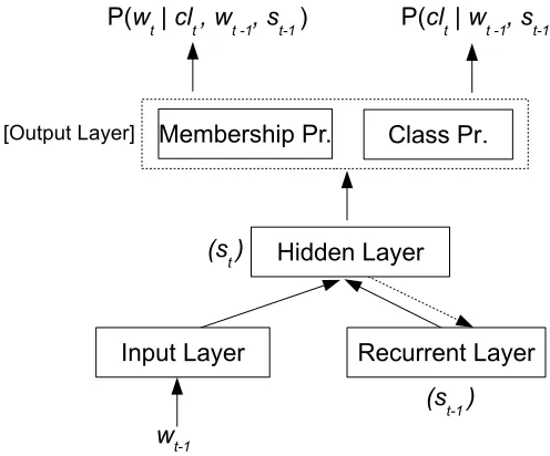
5.3.2 Class-Based RNNLMs . . . 53
5.3.3 Maximum Entropy Features . . . 53
5.3.4 Context-Dependent RNNLMs . . . 55
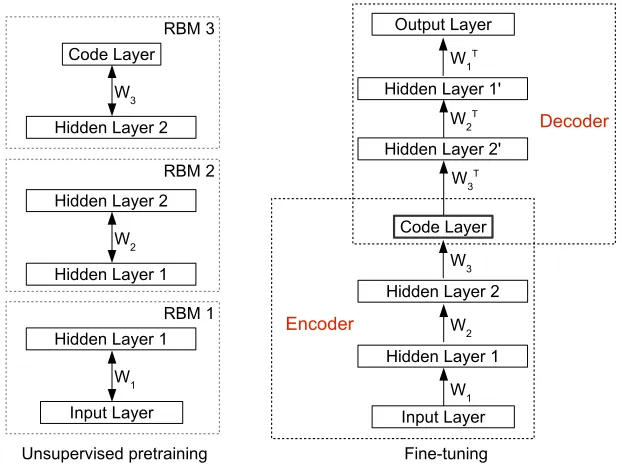
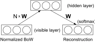
5.4 Deep Autoencoders . . . 55
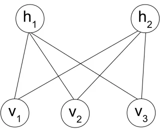
5.4.1 Unsupervised Pretraining . . . 57
5.4.4 Deep Autoencoder for Semantic Context . . . 61
6 Data Description and Baselines 63 6.1 LUNA Human-Machine Corpus . . . 64
6.1.1 ASR Baseline . . . 65
6.1.2 SLU Baseline . . . 66
6.2 LUNA Human-Human Corpus . . . 66
6.2.1 ASR Baseline . . . 67
6.2.2 FrameNet Semantic Parsing . . . 68
6.3 Wall Street Journal Corpus . . . 68
6.3.1 ASR Baseline . . . 69
6.3.2 FrameNet Semantic Parsing . . . 70
7 Joint Models for Spoken Language Understanding 71 7.1 Optimization of Joint LMs for SLU . . . 72
7.1.1 Joint RNNLMs . . . 73
7.1.2 ASR Baseline . . . 74
7.1.3 Baseline for Recognition . . . 75
7.1.4 Re-scoring by Using Joint RNNLMs . . . 76
7.1.5 Parameter Optimization of the Joint Model . . . . 77
7.1.6 Statistical Significance of the Results . . . 78
7.1.7 Conclusion . . . 78
7.2 On-line Adaptation of Semantic Models . . . 79
7.2.1 On-line Adaptation for SLU . . . 80
7.2.2 Instance-Based On-line Adaptation . . . 81
7.2.3 LUNA HM Experiments . . . 84
7.2.4 Statistical Significance of the Results . . . 87
7.2.5 Conclusion . . . 88
7.3 Application of Joint LMs to SLU porting . . . 88
7.3.1 Corpora . . . 89
7.3.2 SMT Systems . . . 91
7.3.3 Style Adaptation . . . 91
7.3.4 Domain Adaptation . . . 92
7.3.5 SLU Performance . . . 93
7.4 Discussion . . . 95
8 Semantic Language Models 97 8.1 The Linguistic Scene . . . 98
8.2 Feature Extraction . . . 101
8.3 SELM Structure . . . 102
8.4 Penn-Treebank Experiments . . . 102
8.5 Wall Street Journal Experiments . . . 105
8.5.1 ASR baseline . . . 105
8.5.2 Re-scoring Experiments – A First Attempt . . . 105
8.5.3 Error Pruning for a Better Semantic Context . . . . 108
8.5.4 Further Analysis . . . 109
8.6 LUNA Human-Human Experiments . . . 112
8.6.1 ASR Baseline . . . 113
8.6.2 Re-scoring Experiments . . . 113
8.6.3 Error Pruning . . . 114
8.7 Discussion . . . 115
9 Deep Encodings for Semantic Language Models 117 9.1 Deep Autoencoders for Encoding Semantic Context . . . . 119
9.1.1 Training Deep Autoencoders . . . 120
9.2 SELM Structure . . . 124
9.3 Wall Street Journal Experiments . . . 125
9.3.1 Experimental Setting . . . 126
9.3.4 Re-scoring Experiments . . . 131
9.3.5 Understanding Performance . . . 133
9.3.6 Combination of Models . . . 134
9.4 Discussion . . . 137
10 Conclusion and Future Work 139
Bibliography 143
6.1 Annotation level statistics for LUNA HM corpus . . . 64
6.2 Splits and statistics for LUNA HM corpus . . . 65
6.3 Baseline ASR performance for LUNA HM corpus . . . 65
6.4 Baseline SLU performance for LUNA HM corpus . . . 66
6.5 Splits and statistics for LUNA HH corpus . . . 67
6.6 Baseline ASR performance for LUNA HH . . . 67
6.7 Frame accuracy on LUNA HH . . . 68
6.8 Target accuracy on LUNA HH . . . 68
6.9 Splits and statistics for WSJ . . . 69
6.10 Baseline ASR Performance for WSJ . . . 70
6.11 Frame accuracy on WSJ . . . 70
6.12 Target accuracy on WSJ . . . 70
7.1 ASR baseline for WER and CER on LUNA HM . . . 75
7.2 Recognition model baseline . . . 75
7.3 Performance of joint RNNLMs . . . 77
7.4 Statistical significance of ASR and SLU optimizations . . . 79
7.5 LUNA HM baseline for semantic model adaptation . . . . 84
7.6 CER lower bounds with the reference transcription on LUNA HM . . . 85
7.7 CER lower bounds with the oracle hypothesis on LUNA HM 86 7.8 CER performance of the on-line adaptation for the LUNA HM corpus . . . 86
7.9 Statistical significance of SLU adaptation on LUNA HM . 87
7.10 SLU porting with style adapted SMT . . . 94
7.11 SLU porting with domain adapted SMT . . . 94
8.1 Word prediction example with semantic language models . 100 8.2 Perplexities on the Penn-Treebank . . . 104
8.3 Baseline ASR Performance for WSJ . . . 105
8.4 WSJ re-scoring performance with full semantic context . . 107
8.5 SELMs with error pruning . . . 109
8.6 WSJ erroneous frame pruning statistics . . . 110
8.7 SELM on Frames with various error pruning rates . . . 112
8.8 Baseline ASR for LUNA HH . . . 113
8.9 Re-scoring on LUNA HH with SELMs . . . 114
8.10 Error pruning for LUNA HH . . . 115
9.1 Baseline ASR Performance for WSJ . . . 126
9.2 Re-scoring with semantic encodings . . . 132
9.3 Re-scoring with interpolated SELMs . . . 136
1.1 A typical spoken dialogue system . . . 2
2.1 IOB representation . . . 15
4.1 A typical ATIS system . . . 34
4.2 Semantic frames in ATIS . . . 34
4.3 An instantiation of a semantic frame . . . 35
5.1 Neural network diagram of the linear discriminant function 44 5.2 Neural network diagram for multi-class classification . . . . 45
5.3 Feed forward neural network language model architecture . 47 5.4 RNNLM architecture . . . 52
5.5 Backpropagation through time (BPTT) . . . 52
5.6 The class-based RNNLM architecture . . . 54
5.7 The context dependent RNNLM architecture . . . 55
5.8 Deep autoencoder . . . 56
5.9 Restricted Boltzmann machines . . . 57
5.10 Contrastive divergence . . . 59
5.11 Constrained Poisson model . . . 61
7.1 SLU Module for Joint Models . . . 72
7.2 Joint RNNLMs . . . 74
7.3 Parameter optimization for joint RNNLMs . . . 78
7.4 Distribution of concepts in the LUNA HM corpus . . . 81
7.5 Instance retrieval process for SLU systems . . . 82
7.6 The diagram of instance-based on-line adaptation scheme . 84 7.7 Test-on-Source SLU porting pipeline . . . 90
8.1 Linguistic scene for a Penn-Treebank sentence . . . 99
8.2 Semantic feature extraction for SELMs . . . 101
8.3 SELM structure for direct semantic features . . . 103
8.4 SELM re-scoring diagram . . . 107
8.5 Error pruning analysis on WSJ . . . 111
9.1 Scatter plot of WER versus Target error rate. . . 118
9.2 Deep autoencoders used for the semantic context . . . 121
9.3 Unsupervised pretraining of the semantic autoencoder . . . 122
9.4 Fine-tuning of the semantic autoencoder . . . 123
9.5 SELM structure for deep semantic encodings . . . 125
9.6 The SELM re-scoring diagram with semantic encodings . . 127
9.7 Histogram of frame encodings . . . 129
9.8 Histogram of target encodings . . . 130
9.9 Joint TER and WER performance of the SELMs. . . 131 9.10 Detailed understanding performance with reference encodings134 9.11 Detailed understanding performance with ASR encodings . 135
Introduction
“A computer would deserve to be called intelligent if it could deceive a human into believing that it was human.” Alan Turing
Alan Turing, after the invention of digital computers brought the possibility of thinking machines [124] to the agenda. He designed a game called “imitation game”, in which a human interrogator asks questions to two players, a machine and a human, to find out which one is the human and which one is the machine. Turing designed the game so that all the information that is passed between the interrogator and the players is through typing. He must have set the communication in this way, probably because at the time, machines communicating through natural speech were seemed infeasible. However, 65 years after Turing designed the imitation game, we can talk about intelligent systems that can recognize and understand human speech.
Still far from being intelligent in the sense Turing implies1, these
ma-1A state-of-the-art spoken dialog system may not be able deceive a human, since by putting a little
effort one can easily break a spoken dialog system.
2
chines started to take an important role in our lives with the increasing use of mobile devices. Among these systems, intelligent personal assistants may be among the most widely used applications, which can communicate through speech. Also, voice search is very satisfactory and efficient, espe-cially on mobile phones where typing is more error prone and cumbersome. This thesis concentrates on the two modules of spoken dialogue systems (SDS) and spoken language systems (SLS): the automatic speech recogni-tion (ASR) and the spoken language understanding (SLU). A diagram of a typical SDS system is given in Figure 1.1 [89].
Figure 1.1: A typical spoken dialogue system. The typical system uses a cascaded archi-tecture.
ASR is the problem of recognizing what words are uttered by the user. ASR systems base their hypotheses on two different information sources which work in combination: acoustic models and language models. Acous-tic models focus on the recognition of the speech sound sequences, and language models (LMs) estimate the probability of word sequences. This thesis focuses on the LM component of the ASR module.
component that understands what the user expects from the system. In this way, the system could act accordingly to satisfy user’s needs.
1.1
Motivation
Most often the two problems, ASR and SLU are approached separately when building SLS as shown in the cascaded architecture in Figure 1.1. First an ASR module is trained and it is optimized for the recognition performance. Then an SLU module that uses the output of the ASR is trained and optimized for the understanding performance. However, as it has been pointed out many times, the hypothesis that gives a better recognition performance does not always yield a better understanding per-formance [108, 127, 38]. If the end goal of SLS is to understand what the user means and respond accordingly, both modules can be optimized jointly such that the system “understands better what it recognizes” and “recognizes better what it understands”.
We believe that LMs that satisfy lexical and semantic constraints jointly would have a better joint performance of recognition and understanding. Therefore, we focus on joint LMs which are constrained by lexical and semantic structures at the same time.
1.2
Contribution of the Thesis
4 1.3. PUBLICATIONS RELEVANT TO THE THESIS
We show how to train and optimize joint LMs for recognition and under-standing. The second model is the “semantic LM” that uses features that are based on the theory of frame semantics [46]. We train semantic LMs by using features extracted from the semantic context. Also, we introduce the use of deep autoencoders to extract more robust semantic features.
This thesis makes the following contributions:
• Training of joint LMs by using lexical and semantic information and optimizing LMs for recognition and understanding.
• On-line adaptation of joint LMs for improving the understanding per-formance.
• Application of joint LMs to cross-language SLU porting.
• Training semantic LMs by exploiting the theory of frame semantics.
• Noisy representation of semantic (linguistic) scene by means of deep autoencoders.
1.3
Publications Relevant to the Thesis
The following publications are relevant to this thesis. They are revised and extended in the preparation of the thesis.
• Bayer A.O. and Riccardi G., “Joint Language Models for Auto-matic Speech Recognition and Understanding”, December 2 - 5, 2012, IEEE Workshop on Spoken Language Technology (SLT 2012), Miami, Florida, USA. [5]
• Stepanov E., Kashkarev I., Bayer A. O., Riccardi G. and Ghosh A., “Language Style and Domain Adaptation for Cross-Language Port-ing”, December 8 - 12, 2013, IEEE Workshop on Automatic Speech Recognition and Understanding (ASRU 2013), Olomouc, Czech Re-public. [119]
• Bayer A.O. and Riccardi G., “Semantic Language Models for Au-tomatic Speech Recognition”, December 7 - 10, 2014, IEEE Work-shop on Spoken Language Technology (SLT 2014), South Lake Tahoe, USA. [7]
• Bayer A.O. and Riccardi G., “Deep Semantic Encodings for Language Modeling”, September 6 - 10, 2015, Interspeech 2015, Dresden, Ger-many. [8]
1.4
Structure of the Thesis
This thesis is structured as follows.
Chapter 2 gives an overview of the ASR and SLU modules and discusses the problems that are addressed in this thesis.
Chapter 3 describes the details of statistical language modeling. The chapter starts with the introduction of the n-gram models and also presents the advanced LM models that uses neural network architectures.
Chapter 4 introduces the problem of spoken language understanding and discusses meaning representations. In addition, it presents computational models for spoken language understanding.
Chapter 5 describes the computational models that are used in this thesis. This chapter is devoted to neural network architectures.
6 1.4. STRUCTURE OF THE THESIS
Chapter 7 describes the training of joint LMs and their optimization for recognition and understanding. Also, on-line adaptation of these semantic models are presented. Finally, applications of joint LMs to cross-language SLU porting is described.
Chapter 8 introduces semantic LMs that are based on the theory of frame semantics. This chapter presents which semantic features are ex-tracted and how these features are integrated to LMs to obtain an accept-able performance.
Chapter 9 presents the use of deep autoencoders for high-level semantic encodings that can be used by semantic LMs.
Background and Relevant Problems
Using speech as the medium of human-computer interaction enables users to communicate easily with computer systems. However, this introduces many research challenges for building spoken language systems (SLS) that function successfully. One of the main problems related to SLS is the recognition of what the user says, namely, automatic speech recognition (ASR). Another main problem is theunderstanding of what is being meant. Although these two problems may seem like two separate problems, in this thesis, we show that both recognition and understanding may benefit from each other and can be approached jointly.
2.1
Automatic Speech Recognition
The recognition problem aims at correctly transcribing every utterance it encounters. Therefore, the main goal of an ASR system is to increase the transcription performance of each word the user utters. The first auto-matic speech recognizer were built in 1950s for the recognition of digits that were spoken by a single individual [33]. Therefore, it was a speaker independent system. This first device could be adapted to another individ-ual by performing manindivid-ual analysis on that individindivid-ual’s speech, and it could recognize digits by using spectral resonances of the vowels. The foundation
8 2.1. AUTOMATIC SPEECH RECOGNITION
of statistical speech recognition, which the current systems are based on, was introduced in 1970s by Jelinek [67] and Baker [4].
The statistical speech recognition approach models the speech recogni-tion problem as follows [68]. A recognizer hypothesis is a string of words,
W, which are drawn from a finite vocabulary based on some acoustic evi-dence A. The word string ˆW, that maximizes the conditional probability of word strings given that acoustic evidence, P(W|A) is the hypothesis that the recognizer searches for:
ˆ
W = arg max
W P(W|A)
Using the Bayes’ formula of probability theory, the above equation can be written as:
ˆ
W = arg max
W
P(W)P(A|W)
P(A) (2.1)
The denominator in equation 2.1 can be ignored during maximization for a given input utterance. Therefore, a statistical speech recognition system uses two knowledge sources:
1. P(W): the probability of a word sequence in a language and it is computed by a “language model”
2. P(A|W): the probability of the acoustic observations given a word sequence which is computed by an “acoustic model”.
2.1.1 Acoustic Model
Acoustic models are not within the scope of this thesis, therefore they will not be treated in detail. A good overview of traditional acoustic modeling can be found in [135]. Traditionally, acoustic models are based on hidden Markov models (HMMs) that model each phoneme in the language. The phonemes can also be modeled considering the preceding and the succeed-ing phonetic context, in which case they are called “context-dependent phonemes”.
The current improvements in training deep neural networks have been resulted in significant improvements also in acoustic modeling. An overview about acoustic models based on deep neural networks can be found in [57, 55]. However, in this thesis we employ the traditional HMM acoustic models with more recent techniques that Kaldi [105] speech recog-nition toolkit provides.
2.1.2 Language Model
Language models (LMs) estimate the probability of occurrences of word sequences in that language. Therefore, they play an important role dur-ing the search for the most likely hypothesis. Chapter 3 gives a detailed overview of statistical language modeling. In this section we focus mainly on the problems related to the current approaches, and our approach to language modeling.
Currently, the most widely used LMs are n-grams, because they are simple models with good baseline performance. N-grams estimate prob-abilities of words by simply counting them in a fixed history, i.e. they assume that the probability of a word is only dependent on the previous
10 2.1. AUTOMATIC SPEECH RECOGNITION
P(wi|hi) ≈ p(wi|wi−n+1,· · · , wi−1) (2.2)
In this respect, n-gram LMs are based on limited size of words occurring together. They treat words as a sequence of symbols and do not exploit the fact that they model a language [109]. Also, one of most important weaknesses of n-grams is the assumption that a word only depends on pre-vious n−1 words and it is independent of the other words [109]. Therefore it is trivial that n-grams fail to capture long-range dependencies that occur naturally in language.
Bellegarda [10] refers to this problem as thelocality problem and explains the problem with the following example. Consider that the LM is trying to predict the word “fell” from the word “stocks” in the following sentences:
stocks fell sharply as a result of the announcement (2.3)
stocks, as a result of the announcement, sharply fell (2.4)
In Sentence 2.3 “fell” can be predicted with a bi-gram LM. However, in 2.4 a 9-gram model would be needed for this prediction which is not feasible. In addition, one can embed more words in between the commas in 2.4 without making the sentence ungrammatical, in this case even a 9-gram would not be sufficient. Hence, models that are based on fixed histories cannot handle long-range dependencies.
The locality problem can be solved by extending the span of the LM to handle the long-range dependencies of the language (span extension). There are two linguistically motivated approaches to extend the span. The first approach is to use the structural information, i.e. the syntax and the second one is to use the semantic information.
to parse the word lattice that is generated by the ASR [27]. In [137], LMs are trained by generating syntactically plausible sentences by using a natu-ral language component. Jurafsky et al. [71] use stochastic CFGs (SCFGs) to extend the corpus for training and interpolates SCFG probabilities with bi-gram probabilities. Chelba et al. [24] use a dependency grammar frame-work with maximum entropy models to constrain word prediction by the linguistically related words in the past. The most important instance of LMs that use syntactic structure is presented in [25]. This model incremen-tally parses hypothesis in a left-to-right manner and assigns a probability to a word considering its parses. However, structured LMs rely on syntactic parsers, therefore, affected by the errors made by the parser [9].
The problem of handling long-range semantic dependencies is ap-proached by trigger pairs in Lau et al. [82]. In this approach, signifi-cantly correlated word sequences are considered as trigger pairs and the occurrence of a triggering sequence causes the probability estimate of the triggered sequence to change. The trigger pairs are modeled by means of feature functions of maximum entropy models. The identification of trig-ger pairs is an issue and in [110] it has been shown that self trigtrig-gers are powerful and robust. Bellegarda [10, 11] applies latent semantic analysis (LSA) to LMs for handling long-range semantic dependencies. LSA [35, 16] is used as an indexing mechanism in information retrieval, where the span of the history is a document which is larger than a sentence.
In this thesis, we consider incorporating semantic relations in LM by using the theory of frame semantics [46]. This approach applies a linguistic semantic theory to language modeling and constructs a linguistic scene by using the information coming from frames evoked in the utterance.
12 2.1. AUTOMATIC SPEECH RECOGNITION
when one wants to model a joint distribution between many words that are represented by discrete random variables. In addition, this kind of representation never considers the similarity between words [14]. For a traditional LM a cat to a dog is no more similar than a cat to a room. One of the solutions to this problem is to represent words in a continuous space, such that each word is represented with an m dimensional vector and these vectors are more closer to each other as the words they represent are more similar. As proposed by Bengio et al. [14], in this approach, each word is associated with a distributed word feature vector and joint probabilities of word sequences are expressed in terms of these feature vectors.
The problem of “curse of dimensionality” is solved by using distributed word representations, where each word is represented by a feature vec-tor [14] on a continuous space. Bengio et al. [14] introduce how LMs that uses distributed representations are modeled, and how these representa-tions are learned by a feed-forward neural network. They have shown significant improvements in perplexity. Schwenk [116] uses neural network LMs for re-scoring multiple ASR hypotheses. Distributed representations have also attracted attention and have been applied to various natural language processing problems [28], in which they were also called “word embeddings”.
Another significant improvement in the recognition performance is ob-tained by the use of recurrent neural networks (RNNs) [96, 80, 94]. RNNs use recurrent connections, which resemble a short-time memory that re-members the state of the model, in this way they can model theoretically infinite histories i.e. long-range dependencies.
2.1.3 Evaluation of ASR Systems
systems, rather than outputting a single hypothesis (1st-best hypothesis), can output multiple hypotheses by using lattices, or n-best lists extracted from these lattices. These lattices or n-best lists can then be re-scored by different models to improve the performance. The evaluation of ASR can be done over the 1st-best or over the oracle hypothesis, which is the best hypothesis in the lattice with respect to the reference transcription.
The statistical speech recognition uses the noisy channel approach. In this approach, the system may make three kinds of errors [2]:
1. : Deletions (D): The hypothesis of the system misses some of the words.
2. : Insertions (I): The hypothesis of the system inserts some extra words.
3. : Substitutions (S): The hypothesis of the system misrecognizes some words and confuses them with similar words.
After the hypothesis of an ASR system is aligned with the reference transcription, these errors are computed and the overall error of the system, word error rate (WER), is calculated as in Equation 2.5, where N refers to the number of words in the reference transcription.
W ER = D +I +S
N (2.5)
2.2
Spoken Language Understanding
14 2.2. SPOKEN LANGUAGE UNDERSTANDING
However, in general it is a harder problem, because of the noisy nature of speech in terms of the ASR word error as well as the variability of the ungramaticality of the conversational speech. [34].
The term SLU defines a very broad research area, the possible set of problems that can be considered in the scope of SLU contains intent deter-mination, spoken utterance classification, topic identification, and speech summarization. This thesis focuses on the semantic frame-based SLU, which is one of the main building blocks of spoken language systems. Semantic-frame-based SLU works on a task specific limited domain which is usually defined by an ontology and aims at correctly recognizing the frames evoked and correctly filling the slots of these frames [130].
As stated in Wang et al. [130], the studies on SLU were started in 1970s with the Defense Advanced Research Projects Agency (DARPA) tasks on speech understanding and resource management. The interest in SLU re-search accelerated with the evaluations on the Air Travel Information Sys-tem (ATIS) which was also sponsored by DARPA in 1990s [106]. In the ATIS domain the SLU task is to respond to user queries about air travel in-formation which are in spontaneous speech. The system responds to queries by converting these queries to SQL statements and by retrieving the in-quired information. Two different approaches emerged from these studies, knowledge-based approaches and statistical approaches. Knowledge-based approaches are based on hand-crafted grammars and not in the scope of this thesis. On the contrary, we focus on statistical systems that can learn from annotated data which are more robust and scalable [130].
2.2.1 Meaning Representation
filled with the required information. For instance, the following sentence in the ATIS domain triggers two frames: “Show me flights from Seattle to Boston” [129].
In addition to the semantic frame representation, the meaning can also be represented as a sequence of basic units. [104] uses keyword-value pairs, (kj, vj), where keywords (kj) represent the conceptual categories like
destination city and values (vj) are the words which were assigned to these
categories like Boston in the above example. This representation is also called attribute-value pairs or flat concept representation. We adopt the attribute-value pair representation in the scope of this thesis.
The SLU models used in this thesis use the flat concept representation with in/out/begin (IOB) representation to handle the concepts mappings that span multiple words. In this approach, the concept tags have addi-tional attributes; “-B” marks the beginning of the concept alignment, and “-I” marks the rest of the alignment. Figure 2.1 gives an example of this representation from the Italian LUNA corpus [41].
Figure 2.1: The flat concept representation with (IOB) representation.
16 2.2. SPOKEN LANGUAGE UNDERSTANDING 2.2.2 Statistical SLU
The SLU problem can also be approached as a sequence labeling problem i.e. the problem of labeling a sequence of words with the correct concept tags. A comparison of various statistical models are given in [53]. The statistical approach can be a generative approach or a discriminative ap-proach. In this thesis we have used the generative approaches that are based on stochastic finite state transducers (SFSTs) [107]. and discrimina-tive approaches that are based on conditional random fields (CRFs) [81]. SFSTs model finite state transducers for making alignments between word sequences and concepts [107] by modeling the joint probability P(W, C), where W represents the word sequence and C represents the concept sequence. CRFs, on the other hand, model the conditional probability
P(C|W) by log-linear models with feature functions. CRFs perform sig-nificantly better than SFSTs [53].
The current state-of-the-art uses neural network models that exploit the distributed word representations as in language modeling [122, 90, 133, 132, 131]. Using distributed word representation improves the performance of SLU in general.
2.2.3 Using Multiple Hypotheses
machines is given in [40].
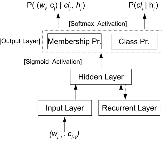
In this thesis, we employ a similar approach to [136]. We use joint neural network LMs that are trained on word-concept pairs (joint LMs) to re-score the output of a baseline SLU model that is built by SFSTs and CRFs. We also address the issue of adaptation of this joint model to the context of the utterance.
2.2.4 Cross-Language SLU porting
Cross-language porting is the problem of transferring the semantic knowl-edge obtained in one language (the source language) to a new language (the target language) when there is no semantic annotation available for the target language [65, 117]. Cross-language porting uses statistical ma-chine translation (SMT) for translating and aligning the resources. The methodology is divided in two categories with respect to the direction of translation: Test-on-Source and Test-on-Target [64]. Test-on-Source uses SMT to translate the utterance to the source language and uses the SLU model in the source language to extract the semantic representation. Test-on-Target, on the other hand, first transfers the semantically annotated resource to the target language and builds an SLU model on the target language.
Statistical Language Modeling
Statistical language models, which will be referred to as language mod-els (LMs) in this thesis, are one of the knowledge sources ASR systems. LMs estimate the probability of utterances in a language by capturing the statistical regularities in that language.
The problem of estimating the probability of an utterance, P(U) is formulated as given in [68]:
The transcription of an utterance U is denoted by W as a sequence of words which are elements of a finite vocabulary V:
W = w1, w2, w3, . . . , wn ∀wi ∈ V
The probability of W is factorized as in Equation 3.1. The preceding words (w1, w2, . . . , wi−1) that the current word (wi) is conditioned on are
referred to as thehistory. Histories may be further mapped into equivalence classes. This mapping leads to an approximate but a simple probabilistic model which would otherwise suffer from data sparseness.
P(w1, w2, w3, . . . , wn) = n Y
i=1
20 3.1. N-GRAM LMS
3.1
N-gram LMs
The idea of having equivalence classes on histories leads to the most com-monly used LMs, n-gram LMs. In n-gram LMs, equivalence classes are constructed based on the most recent words in the history. Therefore, n-gram models use the most recent n− 1 words to build the equivalence classes. Hence, n-gram LM is represented as in Equation 3.2.
P(w1, w2, w3, . . . , wn) ≈ n Y
i=1
P(wi|wi−n+1, . . . , wi−1) (3.2)
Each factor in Equation 3.2 estimates a probability of each word, wi,
in the utterance given a limited window size of n − 1 words. As can be seen, n-gram LMs make the independence assumption that a word is only dependent on the previous n−1 words. These probabilities may be estimated by taking the relevant counts in the training corpus [52]. The maximum likelihood estimates of tri-grams are given as in Equation 3.3, where C(x) denotes the count of the n-gram x.
P(wi|wi−1, wi−2) =
C(wi−2, wi−1, wi) C(wi−2, wi−1)
(3.3)
3.2
Smoothing
In this section, an overview of some of the important smoothing techniques are given, a more detailed overview of various smoothing techniques can be found in [26].
Katz [72] proposes the idea of redistributing the over-estimated observed n-gram probabilities to the n-grams that do not occur. This is based on Good-Turing formula [51]. Assume thatnr denotes the number of n-grams
that occur in the corpus r times. The count is discounted to r∗ or disc(x), as seen in Equation 5.1.
disc(x) =r∗ = (r + 1)nr+1
nr
(3.4)
Katz smoothing distributes the discounted amount to the n-grams that are never seen. Therefore, the discounted counts, r∗, are used when estimating the probabilities for seen n-grams. The probabilities for unseen n-grams are given by backing-off to a lower order n-gram. The Katz probability estimates are given in Equation 3.5, where α(x) is a normalization factor for obtaining a probability distribution.
PKAT Z(wi|wi−n+1, . . . , wi−1) =
disc(wi−n+1,...,wi−1,wi)
C(wi−n+1,...,wi−1) if C(wi−n+1, . . . , wi−1) > 0
α(wi−n+1, . . . , wi−1)PKAT Z(wi|wi−n+2, . . . , wi−1) otherwise
(3.5)
22 3.3. CLASS-BASED LMS
for a word that occurs in lower number of contexts. Kneser-Ney smoothing uses a single discount, D, which is optimized over a held-out set. Kneser-Ney smoothing can be described by the following formula in Equation 3.6 for a bi-gram model [52], where |{v|C(vwi) > 0}| represents the number of
distinct context wi occurs in. The factor α(x) is a normalization factor for
obtaining a probability distribution.
PKN(wi|wi−n+1) =
C(wi−1,wi)−D
C(wi−1) if C(wi−1, wi) > 0
α(wi−1)P|{v|C(vwiy)>0}|
w|{v|C(vw)>0}| otherwise
(3.6)
Chen and Goodman [26] improve Kneser-Ney smoothing by interpolating higher order and lower order counts rather than backing-off to a lower order count when the higher order count is not found. Therefore, interpolated models combine higher order and lower order counts at every occasion. The interpolated Kneser-Ney smoothing for a bi-gram model is given in Equation 3.7.
PIKN(wi|wi−n+1) =
C(wi−1, wi)−D C(wi−1)
+λ(wi)
|{v|C(vwiy) > 0}| P
w|{v|C(vw) > 0}|
(3.7)
Chen and Goodman [26] make further improvements to the interpolated Kneser-Ney smoothing by using multiple discounts; one for single counts, one for double counts, and one for triple or more counts. This is referred as the modified Kneser-Ney smoothing and shown to be the best smoothing technique for large data sets. In this thesis, we have used this smoothing technique when training n-gram models.
3.3
Class-Based LMs
can be calculated for unseen histories based on these classes [21]. The class-based n-grams use a partition function, which maps a word, wi into
a class, ci and they are defined by Equation 3.8.
P(wn|wn−1, . . . , w1) = P(wn|cn)P(cn|cn−1, . . . , c1) (3.8)
The clustering on words can be performed by using a knowledge base or by using data-driven techniques. The knowledge-based approaches may use part-of-speech (POS) tags or even hand-crafted classes like “DATE”, “NAME”, “COMPANY”, etc. [66, 56]. Data-driven approaches cluster words to minimize the overall perplexity of the corpus by a greedy ap-proach [21, 75]. It has been shown that data-driven apap-proaches outperform classes based on POS tags [102].
Neural network LMs (NNLMs) may also use class-based factorization of the probability estimates. The most important reason for that is the training complexity of NNLMs, especially when the vocabulary size is very large [97]. In the NNLMs we have used in this thesis, we use word classes that are based on the unigram frequencies of the words [97], our main pur-pose to use classes is to reduce the computational complexity of NNLMs.
3.4
Maximum Entropy LMs
The principle of maximum entropy models is to find the most uniform distribution, i.e., the distribution that maximizes the entropy that is con-sistent with all the constraints that are imposed on the model [15]. The constraints are imposed on the model by defining binary feature functions orfeatures, fi. These features return 1 if a constraint is satisfied and 0
24 3.4. MAXIMUM ENTROPY LMS
P(wn|wn−1, . . . , w1) =
exp(P
kλkfk(wn, wn−1, . . . , w1)) z(wn−1, . . . , w1)
(3.9)
The denominator is a normalization factor that is given by Equa-tion 3.10.
z(wn−1, . . . , w1) = X
w
exp(X
k
λkfk(w, wn−1, . . . , w1)) (3.10)
The weights, λk, are learned by using a learning algorithm like
general-ized iterative scaling [31]. The features may represent n-grams, caches, and skipping models. Maximum entropy models are reported not to improve much with respect to comparable interpolated n-gram models [52]. And also they are reported to be very time consuming to train and test.
One of the contributions of maximum entropy LMs is the use of trigger pairs as features [82]. Trigger pairs are defined by a trigger function be-tween words, therefore if a word sequence A is significantly correlated with a word sequence B, they constitute a trigger pair. Then, Ais referred to as the trigger and B as the triggered sequence. Rosenfeld [110] reports that self triggers are very powerful and robust. Also trigger pairs of frequent words have more potential than the trigger pairs of infrequent words. Trig-ger pairs are determined by using the average mutual information between the trigger and the triggered sequence. Trigger pairs are very effective to handle the long-range dependencies.
3.5
Structured LMs
Structured LMs aim at exploiting the syntactic structure of utterances to handle long-range dependencies better than a fixed context. The first attempts are based on using context free grammars (CFGs) [27, 137, 71]. The main contribution of structured LMs is started with Chelba et al. [24] in which a dependency grammar framework with maximum entropy models is used to constrain the word prediction by the linguistically related words in the past.
26 3.6. SEMANTIC LMS
3.6
Semantic LMs
Semantic LMs consider the semantic dependencies in the language. One of the approaches that incorporates semantic information into LM is the topic model [49, 114]. The topics may be selected from a hand-crafted set or can be learned by data-driven approaches. Topic LMs model the probability of a word in a topic and do not consider the local structure of the language. Therefore they are combined with n-gram models.
Trigger pairs as introduced in Section 3.4 may also be considered as a form of a semantic LM since they consider the significant correlations between trigger pairs. The performance of trigger pairs are dependent mostly on the selection of pairs.
Bellegarda [10, 11] uses latent semantic analysis (LSA) to extend the trigger pair approach. LSA [35, 16] is used as an indexing mechanism in information retrieval, it maps the discrete space of words and documents1 to the same continuous space. Therefore, each word and document is represented as a vector in this space. A word-document matrix, in which each column represents a document and each row represents a word, is constructed by populating the matrix values by normalized counts of the words in the documents. The normalization is done with respect to the number of documents in which the word occurs. Because of computational requirements, singular value decomposition is applied to this matrix. The final representation conceptually represents each word and document as a linear combination of abstract concepts, which is very similar to the distributed representations the neural network LMs use. At the final step, LMs are modeled over the LSA history of the word. Combining LSA with n-gram models resulted in significant improvements in perplexity and word error rate [10, 11].
3.7
Neural Network LMs
N-gram LMs represent the words on a discrete space where it is not possible to model any relationships between words, regarding their position in this space. Neural network LMs (NNLMs) address this issue which suffers from curse of dimensionality. During training, NNLMs learn distributed representations, i.e., continuous valued vectors of words. Hence, NNLMs, associate a distributed representation (also known as a word embedding) with each word in the vocabulary and model the joint probability of word sequences over these vectors [14].
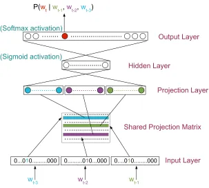
NNLMs are first started to be used in [14] and they were reported to reduce the perplexity. The first application of NNLMs to ASR is presented in [116] which is reported to drop the WER by linear interpolating NNLMs with back-off n-gram LMs. The detailed structure of NNLMs and their training procedure is presented in Chapter 5. The structure of feed-forward NNLMs is given in Figure 5.3 [14].
The input to feed-forward NNLMs is given as 1-of-n encoding, in which the index of the word is set to 1 and the rest is set to 0. The words are mapped to a continuous space by using a shared matrix, the projection matrix. The projection layer concatenates word vectors and it is fully-connected to the hidden layer. The hidden layer uses a non-linear activation function (the sigmoid function or tanh) and it is fully-connected to the output layer. The output layer, outputs a probability estimate for every word in the vocabulary by using a softmax function. The main complexity comes from the connections between the hidden layer and the output layer. Therefore, the vocabulary size plays a crucial rule in the complexity of NNLMs.
28 3.7. NEURAL NETWORK LMS
words and NNLMs are trained only for this shortlist. During prediction, NNLMs are used only for predicting probabilities of the words that are in the shortlist, the probabilities for the other words are estimated by using n-gram models. The hierarchical NNLM [101, 100] adopts a binary clustering of the words at the output layer to reduce the computational complexity. Structured output layer NNLMs [83, 84] use another tree representation at the output layer. In this approach, all words except a shortlist of words are clustered based on the distributed representations learned at the projection layer. A class-based output layer is presented in [97]. In this approach, word probabilities are factorized into class membership probabilities and class probabilities. The clustering is done based on the unigram frequen-cies of the words. All clustering techniques degrade the performance of NNLMs, however, for large vocabularies they make NNLMs feasible. In this thesis, we use the class-based output approach.
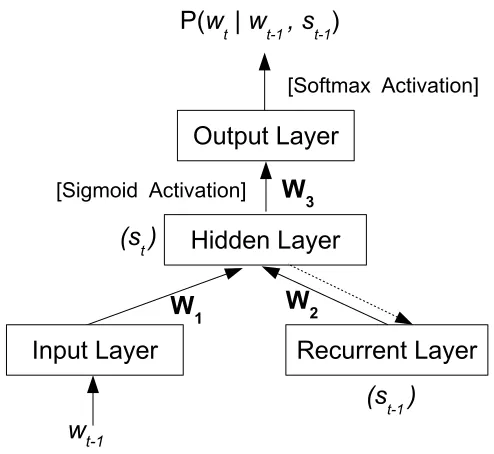
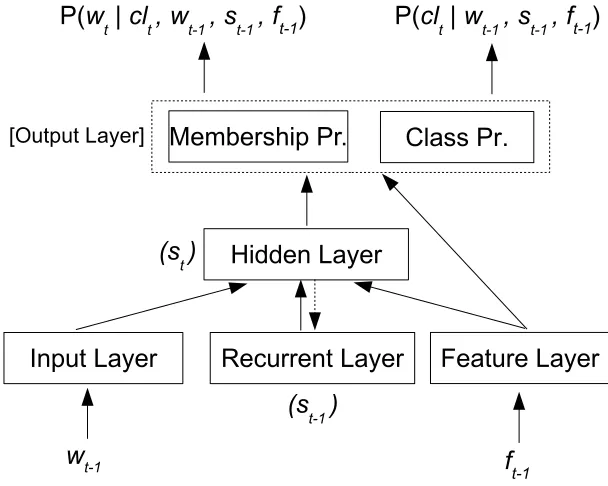
Feed-forward NNLMs are based on fixed histories, therefore they also suffer from the problems related to fixed histories. Recurrent NNLMs (RNNLMs) [96, 93] overcome this problem by using recurrent connections, which represent the state of the network. This can be thought of as a short-term memory, which in theory, enables the network to model infinite size of histories. RNNLMs are shown to improve perplexities and WERs better than any feed-forward NNLM [94]. In [92], a feature layer is added to RNNLMs, where topic features are used as additional context to the NNLM. In addition, Mikolov et al. [91] present the training of maximum entropy features jointly with the RNNLM. The maximum entropy features are over n-grams and they are implemented with a hash-based implementa-tion, where n-grams are clustered based on hash functions. The RNNLMs that are trained jointly with maximum entropy models are referred to as RNNME.
because the gradients of errors become smaller and smaller; this is known as the vanishing gradient problem [13]. Mikolov et al. [95] address the problem of vanishing gradients by comparing Long Short Term Memory (LSTM) networks [62] withstructurally constraint recurrent networks (SCRNs) that have a hidden layer that is designed to capture long term dependencies. Authors report that the performance of the two architectures are similar and they outperform RNNLMs.
3.8
Combining LMs
The most widely used method for combining LMs is the linear interpolation method given by Equation 3.11.
p(w|h) =X
i
λipi(w|h) (3.11)
The mixture weights λi sum to 1 so that it gives a probability
distribu-tion. The weights are adjusted over a development data by minimizing the overall perplexity either by using the expectation maximization algorithm or empirically over WER.
linear interpolation can also be applied for combining LMs. Log-linear interpolation has the following form given in Equation 3.12 [73].
p(w|h) = 1
Zλ(h) Y
i
pi(w|h)λi (3.12)
Log-linear interpolation does not impose any explicit constraint over the mixture weights, however, the normalization factor Zλ(h) is needed
30 3.9. EVALUATION OF LMS
In this thesis, we apply linear interpolation to combine multiple neural network language models.
3.9
Evaluation of LMs
LMs are evaluated by using two different metrics. The first one is the measure of how well it captures the unseen data, perplexity. Perplexity is closely related to cross entropy from information theory. The second one measures how well LMs perform in ASR tasks, word error rate (WER), which is the basic evaluation metric for ASR systems.
Perplexity (PPL) is calculated on an evaluation corpus of N words as in Equation 3.13 [52]. Perplexity is proportional to the cross entropy2 of the evaluation corpus given the model. Therefore, the lower the perplexity is, the better the LM models the evaluation data.
P P L = N
v u u t
N Y
i=1
1
P(wi|w1. . . wi−1)
(3.13)
As described in Chapter 2, WER is calculated by first aligning the ASR hypothesis with the reference transcription and then dividing the errors made (insertions, deletions, and substitutions) to the number of tokens in the reference transcription.
Both metrics have advantages and disadvantages. Computing perplex-ity is easy and it correlates with the system performance, however, may mislead the comparison between two models if one relies on future infor-mation. WER, on the other hand, requires a full ASR system and does not discriminate between type of errors. However, it gives an idea about the actual performance of the LM for the specific task at hand.
2Cross entropy is log
Spoken Language Understanding
“The noblest pleasure is the joy of understanding.” Leonardo da Vinci
Language is far more than strings of words. As Fillmore [46] points out, when speakers want to greet someone, they consider the utterance “Good morning, sir.” as one of the options to greet the addressee. Speakers also know that this utterance is appropriate when the addressee is an adult male and only during a certain time in the day. Therefore, utterances have several complexities beyond being composed of lexical units; on one hand they have the function they serve, greeting in this case, and, on the other hand, they have their appropriate context.
Language understanding, in addition to the analysis of compositional meaning of lexical units, deals with finding out the function and the con-text of an utterance. Semantic-frame based understanding addresses the function and the context of an utterance based on the notion of frames.
Spoken language understanding (SLU) is most often performed by us-ing a semantic-frame approach [130]. Its goal is to correctly identify the
32
semantic frames in the utterance and extract the values for the slots asso-ciated to the frames.
The notion of a “frame” [99] is proposed as a data structure to represent knowledge with a stereo-typed situation. In this framework, upon encoun-tering a situation, one selects an appropriate frame from the memory and changes the details if necessary. The frame is represented as a network of nodes and relations. The frame has top levels which are always fixed and low levels which have “slots” that need to be filled by an instance of a situation. The theory of frame semantics is based on the notion of frames and consider semantics as the set of relations between linguistic forms and their meanings [47]. For instance, in a situation where there is a commercial event, i.e., when the commercial event frame is evoked, this frame contains roles or slots like the buyer, the seller, the goods, and the money. The linguistic units that evoke these frames are called lexical units, target words or targets which can be one of the following words, “buy”, “sell”, or “charge” [46]. FrameNet [48] is a project that extracts re-lations about the semantic and syntactic properties of English words from large text by means of manual semantic annotations and automatic pro-cessing. FrameNet project constructs a relational network of frames, and includes the list of lexical units and the frames they evoke with respect to their senses. The following example is taken from the FrameNet project that demonstrates the frame of “Commerce Scenario”:
M y local grocery store raised prices on meat
In this example, the lexical unit or the target word prices evokes the frame “Commerce Scenario”. In this case, two slots of this frame “Seller” and “Goods” are filled with the phrases “My local grocery store” and “meat” respectively.
an overview of frame-semantic parsing is given that is required by the semantic models which are described later in the thesis.
4.1
Spoken Language Understating
Spoken language understanding is the problem of extracting meaning rep-resentations from user utterances [129, 34]. The application domains of SLU are spoken dialog systems, speech information retrieval, and speech translation [34]. SLU and natural language understanding (NLU) is closely related. The focus of NLU is extracting meaning representations from a generic domain written text. On the other hand, SLU focuses on applica-tion specific domains and works on speech signals. The nature of speech brings additional difficulties that are not present in NLU. These difficulties are defined as: [130]
• The syntactic structure of spoken utterances are not well-formed as written-text.
• Disfluencies (hesitations, corrections, or repetitions) occur in speech.
• SLU relies on the ASR output, and ASR errors are propagated to SLU. Therefore, SLU systems must be trained to be robust to this noise.
• Out-of-domain utterance cannot be modeled well.
The research on SLU is started to gain interest with the Air Travel Information System (ATIS) evaluations [106]. ATIS evaluations resulted in systems that process spontaneous speech queries for air travel information and that bring back the relevant information from a database. A typical ATIS system is shown in Figure 4.1 [129].
34 4.1. SPOKEN LANGUAGE UNDERSTATING
Figure 4.1: A typical ATIS system uses a cascaded approach. The SLU uses the ASR hypothesis and produces a semantic representation. This semantic representation is con-verted to a SQL query to retrieve the relevant information from the database.
4.1.1 Semantic Representation
In semantic-frame based SLU, semantic information is represented by se-mantic frames. Sese-mantic frames are similar to the frames in the theory of frame semantics and they contain typed slots that need to be filled with respect to the semantic information. Figure 4.2 gives an example of three frames taken from the ATIS domain [129].
Figure 4.2: Three semantic frames from the ATIS domain. The frames and the database are designed together so that they represent the same information. For example, the flight frame has slots “DCity” which represents the destination city, “ACity” which represents the arrival city, and “DDate” which represents the date of departure. The frames are simplified in this example.
cities and also the departure time. An instantiation of the flight frame for the user query “Show me flights from Seattle to Boston.” is given in Figure 4.3 [129].
Figure 4.3: An instantiation of the “flight” frame with for the user query “Show me flights from Seattle to Boston.”. The departure and arrival city slots are filled respectively.
Semantic frames use a hierarchical approach to represent meaning rep-resentations. Another representation scheme is a simplified attribute-value pair representation or a keyword pair representation [104]. Attribute-value pairs use a flat representation scheme and do not possess a hierarchical structure. For the same user query, “Show me flights from Seattle to Boston.”, we may have the following attribute-value pair representation in the ATIS domain: “(Command DISPLAY) (Subject FLIGHT) (DCity SEA) (ACity BOS). In addition, if an attribute spans multiple tokens of values, in/out/begin (IOB) representation can be used. For instance, in “Show me flights from Seattle to New York” the arrival city “New York” is represented with the following attribute-pairs “(ACity-B New) (ACity-I York)”.
36 4.1. SPOKEN LANGUAGE UNDERSTATING 4.1.2 Evaluation Metrics
The evaluation of SLU is performed on the semantic representation it out-puts. The common evaluation metrics are [130]:
• Concept Error Rate (CER): Also known as slot error rate (SER). It measures the concept/slot performance of the SLU system. SLU hypothesis is aligned with the reference semantic annotation. Inser-tion (I), deletion (D), and substitution (S) errors are determined and CER is computed by Equation 4.1, where N represents the number of concepts/slots in the reference annotation.
CER = I +D +S
N (4.1)
• Slot Precision/Recall/F1 Score: Precision/Recall/F1 scores are also used to assess the slot performance of the SLU system. They are calculated as follows:
P recision = Number of correctly recognized slots
Number of total slots recognized by the system (4.2)
Recall = Number of correctly recognized slots
Number of total slots in the reference annotation (4.3)
F1 = 2×(P recision×Recall)
4.2
Data Driven Approaches to SLU
SLU approaches are categorized into two; knowledge-based approaches and data driven approaches. Knowledge-based approaches use hand-crafted grammars, which are not easy to tune and scale. Data driven approaches, on the other hand, learn SLU models from semantically annotated training examples [130]. This thesis focuses on data driven approaches, therefore, we do not present knowledge-based approaches.
In a statistical framework, the semantic frame-based SLU problem is formalized as finding the most likely semantic representation, ˆC, given a sequence of words, W. It corresponds to finding the semantic representa-tion that maximizes the probability P(C|W).
4.2.1 Generative Models
Generative models, maximize the joint probability P(W, C) by using the training data. They are described by Equation 4.5 [98, 130, 53].
ˆ
C = arg max
C P(C|W) = arg maxC P(W|C)P(C) (4.5)
38 4.2. DATA DRIVEN APPROACHES TO SLU
words which are not assigned to any slots. Therefore, the joint probability of a sequence of words, W = {w1,· · · , wn} and a sequence of concepts C = {c1,· · · , cn} are modeled by the joint probability P(W, C), which is
computed as in Equation 4.6.
P(W, C) =
k Y
i=1
P(wici|wi−1ci−1,· · · , w1c1) (4.6)
Stochastic finite state transducers (SFSTs) are used as a generative SLU model [107]. In this framework, the transducer that models SLU takes words as input and outputs the concept tags. The SLU transducer,
λSLU is composed of three other SFSTs. λW is used for representing the
input, λw2c models all word to concept mappings that are hand-crafted or
learned from a training corpus, λSLM is a language model over the concepts
represented as a SFST. The SLU model, λSLU, which is the composition
of the three SFSTs is given in Equation 4.7.
λSLU = λW ◦λw2c ◦λSLM (4.7)
4.2.2 Discriminative Models
P(C|W,Λ) = exp(
P
kλkfk(C, W))
Z(W,Λ) (4.8)
fk(C, W) denotes the kth feature function that is defined over the
se-quences of words and concepts. Λ = {λ1..., λk..., λn} is a set of parameters
that are learned during training and Z(W,Λ) is the partition function that normalizes the probability distribution. Training CRFs are very inefficient because feature functions are defined over the entire label sequence. Fea-tures functions can be constrained to be defined on the immediate states which makes training and inference more efficient [128].
Feature functions for CRF SLU models are typically n-gram features to capture the relationship between the label and the current and previously observed words, transition features which model the current label with the predicted previous label, and class member features which models the clustering for the words [130]. Trigger pairs are introduced as features to handle long-range dependencies in [69]. They are similar to the trigger pairs introduced in [82].
4.2.3 Neural Network Models
40 4.2. DATA DRIVEN APPROACHES TO SLU
RNNs outperform CRFs, however, for another dataset CRFs outperform RNNs. Yao et al. [133] build models using word embeddings and named entity features; the authors report that RNNs outperform CRFs on the ATIS dataset. In [132], long short-term memory (LSTM) [62] models are used for SLU modeling. LSTM models use a memory cell to store informa-tion and they are reported to model long-range dependencies better than RNNs [132]. Deep belief networks are applied to SLU in [39], and convolu-tional neural networks are jointly trained with CRFs for slot filling [131].
As can be seen, with the increased interest on neural networks, SLU has started to be approached by different architectures of neural networks. The use of distributed representations of words and concepts provide leverage also for the SLU problem.
4.2.4 Using Multiple Hypotheses
In that respect, we use n-best ASR hypotheses and feed it into the baseline SLU model and obtain the multiple SLU hypotheses. Then, we re-score these SLU hypotheses by using RNN models.
4.3
Frame-Semantic Parsing
Frame-semantic parsing is the problem of automatically assigning the frame-semantic structure to natural language sentences. Frame-semantic parsing has been most often applied to written text and in generic domains (e.g. news text). Statistical domain independent frame-semantic parsing is started with the task of “semantic role labeling” in which the semantic roles are defined with frame elements of semantic frames [50]. The CoNLL shared tasks [23] on semantic role labeling also contributed to this research. Although, semantic role labeling deals only with filling frame elements a full pipeline for frame-semantic parsing needs to handle all of the following subtasks [32]:
• Target Recognition: This subtask decides which words evoke se-mantic frames in a sentence.
• Frame Identification: This task identifies the correct frame that a target evokes. Since, a word can evoke more than one frame with respect to the context, this is a multi-class classification task given the frame evoking word.
• Frame Element (Argument) Detection: This task detects which frame elements are filled in the sentence and finds the correct span of the frame elements over the phrases.
42 4.3. FRAME-SEMANTIC PARSING
Neural Network Models
This chapter gives a detailed explanation of the neural network architec-tures used in this thesis. The first section introduces the related termi-nology of neural networks on single layer networks. In Section 5.2, feed forward neural network LMs are presented. Section 5.3 continues with re-current neural network LMs. Finally, deep autoencoders that are used for semantic feature extraction are described in Section 5.4.
5.1
Single Layer Networks
This section presents the building blocks of multi-layer neural networks and introduces the related terminology. The reader may refer to [19] for a detailed explanation of the concepts, from which this section is compiled.
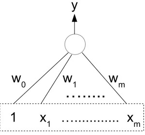
A classification problem on two categories may be performed by using a discriminant function, y(x) such that the value of the function determines which class the m dimensional vector x belongs to. A decision rule as-signs y(x) to class C1 if y(x) > 0 and to class C2 if y(x) < 0. A simple
discriminative function is given in Equation 5.1.
y(x) =wTx+w0 (5.1)
44 5.1. SINGLE LAYER NETWORKS
Figure 5.1: Neural network diagram of the linear discriminant function. The bias w0 is
represented as an additional weight with an input value of 1.
The m dimensional vector w is referred to as the weight vector and the scalar w0 is referred to as the bias. The decision boundary is given by y(x) = 0 and corresponds to a (m − 1) dimensional hyperplane in m
dimensional space. Since this decision boundary is linear, it is appropriate for the classification problems that are linearly separable. The classification that is performed with such a discriminative function is referred to as linear classification.
The linear discriminant function in Equation 5.1 can be represented by a network diagram as given in Figure 5.1. This figure represents the weight vector as the concatenation of the bias w0 with w and the input vector as
the concatenation of 1 with x.
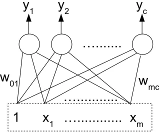
5.1.1 Multi-Class Classification
The classification can be extended tocclasses by using a linear discriminant function yk(x) for each class Ck. Then the decision is made by assigning
the input to Ck if yk(x) > yj(x) for all j 6= k. The linear discriminant
Figure 5.2: Neural network diagram for multi-class classification
yk(x) = m X
i=0
wkixi (5.2)
The weights of the network can be learned by minimizing an error func-tion over training data of size N, X = {x1, . . . ,xN}, where each element, xi is a vector of size m. The target value at node k for the input xi is given by tik. Also we represent the output of node k with the weights w for the input xi as y
k(xi;w). Then the sum-of-squares error function that is
defined over the parameters of the network, is written as in Equation 5.3.
E(w) = 1 2
N X
n=1 c X
k=1
{yk(xn;w)−tnk}2 (5.3)
Then the optimal values of weights can be determined bygradient descent, i.e., by iteratively going over the training data and updating the weights as given in Equation 5.4 for the time step τ + 1. w0kj denotes the initial weights.
w(τ+1)kj = wkj(τ)−η∂E(w) ∂wkj
w(kjτ)
(5.4)
empir-46 5.2. FEED FORWARD NEURAL NETWORK LMS
ically.
5.1.2 Activation Function
The discriminant function given in 5.2 is a linear function of the input, x. A monotonic non-linear function g(.) may also be used. In this case, the function g(.) is called the activation function. A discriminant function that uses an activation function can be given as in Equation 5.5. The decision boundary generated by such a discriminant function is still linear.
yk(x) = g(ak), where ak = m X
i=0
wkixi (5.5)
The sigmoid activation in Equation 5.6 is one of the most widely used non-linear functions because of its nice derivative, and it maps the interval (∞,−∞) onto interval (0,1).
If we want to model the conditional probability distribution P(Ck|x)
that estimates the probability of input xbelonging to class Ck, thesoftmax
function that is given in Equation 5.7 can be used.
g(ak) =
1
1 +e−ak (5.6)
g(ak) =
eak
Pc
k′=1eak′
(5.7)
5.2
Feed Forward Neural Network LMs
Figure 5.3: Feed forward neural network language model architecture. The input layer takes the history by 1-of-n encoding of words. The projection layer, project the word vectors onto a continuous space by using a shared projection matrix. The output layer estimates the probability of the next word. The projection layer is also fully connected to the output layer, however, it is not shown in the illustration.
structure of an n-gram FFLM is given in Figure 5.3. FFLMs usually are composed of four layers.
The input layer represents the words with 1-of-n encoding. In this rep-resentation each word is represented by a vector where only the index of the designated word is set to 1 and the others are set to 0.