DOES A “LIQUIDITY TRAP” EXIST TODAY (2009) AND DOES IT MATTER?
by
STEVEN P. ARTZER
B.S., United States Naval Academy, 1977 M.S., The Naval Post Graduate School, 1982
A THESIS
submitted in partial fulfillment of the requirements for the degree
MASTER OF ARTS
Department of Economics College of Arts and Sciences
KANSAS STATE UNIVERSITY Manhattan, Kansas
2009
Approved by:
Major Professor Dr. Lloyd B. Thomas, Jr.
Copyright
STEVEN P. ARTZER 2009
Abstract
Can stimulative monetary policy be effective when there is a “liquidity trap”? This question surfaced during the Great Depression and is raising its head again today due to the current financial crisis. A definitive answer never materialized for the 1930’s, as differences of opinion between non-monetarist and monetarist economists arose about this issue. This need not be the case today. In this thesis I will first enumerate several different meanings of the term “liquidity trap” and their implications for monetary policy. Then, with data from the Federal Reserve, I will attempt to validate the likelihood of a liquidity trap. I do this for the demand for money and bank liquidity traps. I use regression analysis over a fifteen year period with varying interest rates to determine if the elasticities of demand increase as interest rates fall, indicating a liquidity trap. My use of log linear regressions for both demand for money and bank liquidity traps, using data from the present financial crisis, adds to the evidence supporting the liquidity hypothesis, but does not empirically establish the existence of a liquidity trap.
Following my findings, I detail actions taken by the Federal Reserve and show the subsequent results through the summer and into the fall of 2009. From this, I make a conclusion that the United States is most likely in a liquidity trap and it does matter.
Table of Contents
List of Figures ... vii
List of Tables ... ix
CHAPTER 1 - “Liquidity Trap” ... 1
Liquidity ... 1
Liquidity Trap ... 3
Demand for Money Liquidity Trap ... 3
Money Demand Function ... 4
Money Supply Function ... 6
IS-LM Derivation Method 1 ... 11
The LM Curve ... 11
The IS Curve ... 12
General Equilibrium ... 14
IS-LM Derivation Method 2 ... 15
The IS Curve ... 15
The LM Curve ... 17
General Equilibrium ... 21
Expansionary Monetary Policy ... 22
“Liquidity Trap” ... 23
Bank “Liquidity Trap” ... 25
Reasons Why Banks Hold More Money ... 26
How the Meaning of “Liquidity Trap” Has Changed Over Time. ... 27
Theory Review ... 29
CHAPTER 2 - Is There Evidence of Liquidity Trap? ... 31
Demand for Money “Liquidity Trap” ... 31
Regression Analysis to Investigate Interest Elasticity of Money Demand ... 39
Regression Procedure... 39
Regression Results ... 40
Bank “Liquidity Trap” ... 42
Regression Analysis to Investigate Existence of a Bank Liquidity Trap ... 47
Regression Procedure... 47
Regression Results ... 48
Regression Analysis ... 49
CHAPTER 3 - Actions Taken by the Federal Reserve to Increase Liquidity ... 62
Discount Window Lending ... 62
Term Auction Facility (TAF) ... 63
Swap Lines ... 64
Dollar Liquidity Swap Lines ... 65
Foreign-Currency Liquidity Swap Lines ... 65
Twenty-eight Day Repurchase Agreements ... 65
Term Securities Lending Facility (TSLF) ... 66
Bear Stearns and JP Morgan Chase ... 66
Primary Dealer Credit Facility (PDCF) ... 67
Additional Actions ... 67
Asset-Backed Commercial Paper Money Market Mutual Fund Liquidity Facility (AMLF) ... 67
Commercial Paper Lending Facility (CPFF) ... 68
Money Market Investor Funding Facility ... 68
Term Asset-Backed Securities Loan Facility (TALF) ... 68
Interest Paid on Required Balances and Excess Balances ... 70
Special Liquidity Injections Summary ... 70
CHAPTER 4 - Have the Special Liquidity Injections Worked? ... 72
Indicators of Failure ... 72
Liquidity Program Extensions ... 72
Liquidity Program Scope ... 73
Liquidity Program Targets ... 73
Liquidity Program’s Size ... 73
Borrowing Time ... 73
Swap Lines ... 73
TAF Auctions ... 74
TSLF Auctions ... 74
MMIF ... 74
AMLF ... 75
CHAPTER 5 - Conducting Monetary Policy at Low Interest Rates ... 76
Influencing Expected Future Interest Rates ... 76
Balance Sheet Composition ... 77
Balance Sheet Size ... 77
Federal Reserve Monetary Policy ... 77
Results ... 79
CHAPTER 6 - The Role of Inflationary Expectations ... 80
Irresponsible Monetary Policy? ... 80
Fiscal Policy ... 81
Expectations and Japan’s Liquidity Trap ... 82
CHAPTER 7 - Have U.S. Policy Actions Been Effective? ... 90
CHAPTER 8 - Conclusion ... 96
List of Figures
Figure 1 The Money Demand Function ... 4
Figure 2 Liquidity Preference ... 6
Figure 3 The Money Supply Function ... 7
Figure 4 Money Supply Increases and Interest Rate Falls ... 8
Figure 5 Keynesian Model... 9
Figure 6 Spending and Output Increases ... 10
Figure 7 Method 1 Derivation of LM Curve ... 11
Figure 8 Method 1 Derivation of IS Curve ... 13
Figure 9 Method 1 General Equilibrium ... 14
Figure 10 Keynesian Cross ... 16
Figure 11 Method 2 Derivation of IS Curve ... 17
Figure 12 Liquidity Preference ... 18
Figure 13 Increase in the Money Supply Under Liquidity Preference ... 19
Figure 14 Increase in Income ... 20
Figure 15 Method 2 Derivation of LM Curve ... 21
Figure 16 IS-LM Curve ... 21
Figure 17 Expansionary Monetary Policy ... 22
Figure 18 Aggregate Demand ... 23
Figure 19 IS-LM Liquidity Trap ... 24
Figure 20 Bank Demand for Excess Reserves ... 25
Figure 21 Supply and Demand for Bank Excess Reserves ... 26
Figure 22 Federal Funds Rate ... 31
Figure 23 M2 Money Supply ... 32
Figure 24 Nominal GDP ... 33
Figure 25 Nominal GDP ... 35
Figure 26 Velocity (GDP/M2) ... 36
Figure 28 Money and Interest Rates 2006:1-2009:3 ... 38
Figure 29 Total Bank Reserves ... 43
Figure 30 Excess Reserves ... 43
Figure 31 Amounts of Bank Loans ... 44
Figure 32 Monetary Base ... 45
Figure 33 M2/Monetary Base ... 46
Figure 34 Keynesian View of Bank Demand for Excess Reserves ... 47
Figure 35 Predicted vs. Actual Excess Reserves ... 55
Figure 36 Excess Reserves and Interest Rates ... 56
Figure 37 Scatter Plot 3-Month T-Bill vs. Excess Reserves/DDO ... 57
Figure 38 Scatter Plot 3-Month T-Bill rate vs. Excess Reserves/DDO with Pertinent Points Removed ... 58
Figure 39 Japan’s Inflation Rate ... 82
Figure 40 Japan's Recent Inflation Rate ... 83
Figure 41 Japan’s Interest Rate... 83
Figure 42 Japan Government Budget ... 84
Figure 43 Japan Real GDP Growth Rate ... 84
Figure 44 Japan's Recent Real Growth Rate ... 85
Figure 45 Selected World Domestic Money Aggregates ... 86
Figure 46 Gross Debt to GDP, Japan and Other Nations ... 87
Figure 47 Expected Inflation Rate 1 Year Ahead ... 92
Figure 48 Expected Inflation Rate 5-10 Years Ahead ... 93
Figure 49 Nominal Treasury Yield Curves ... 94
List of Tables
Table 1 Equation of Exchange Variables... 34
Table 2 Estimation of Money Demand Model (January 1994- April 2009) ... 41
Table 3 Estimation of Banker's Liquidity Trap Model Jan 1994-April 2009 ... 49
Table 4 Estimation of Banker's Liquidity Trap Model from Jan 1994-Jul 2007... 51
Table 5 Estimation of Banker's Liquidity Trap Model (Jan 1994-Dec 2007, non log form) ... 52
Table 6 Regressions from Jan 1970-Aug 2008 ... 53
Table 7 Predicted vs. Actual Excess Reserves ... 54
Table 8 Regressions from Jan 1970-Aug 2008 ... 59
Table 9 Regressions from Jan 1970-Aug 2008 less Dec 90, Jan 91, Feb 91, Jan 00, Sept 01, & Aug 07 ... 59
Table 10 Regressions from Jan 1970 – Aug 2008 less Dec 90, Jan 91, Feb 91, Jan 2000, Sep 2001, Aug 2007 for 3% and 4% ... 60
Table 11 Log Regressions from Jan 1970 - aug 2008 less Dec90, Jan 91, Feb 91, Jan 2000, Sep 2001, Aug 2007 for 3% and 4% ... 61
Table 12 Special Liquidity Injections Summary ... 71
CHAPTER 1 - “Liquidity Trap”
Is monetary policy effective when there is a “liquidity trap”? This question surfaced during the Great Depression and is raising its head again today due to the current financial crisis. A definitive answer never materialized for the 1930’s as differences of opinion regarding the cause of the Great Depression between non-monetarist and monetarist economist arose. This need not be the case today. In this thesis I will first enumerate several different meanings of the term “liquidity trap” and their implications for monetary policy. Then, with data from the Federal Reserve, I will attempt to validate the likelihood of a liquidity trap. I will detail actions taken by the Federal Reserve and the subsequent results on the economy. From this, a conclusion can be made on whether the existence of a liquidity trap matters.
Liquidity
Before discussing a “liquidity trap”, the term “liquidity” needs to be understood. It is important to understand the word “liquidity”, because a financial crisis can occur when liquidity disappears. Liquidity has several different meanings. The most common and generalized meaning refers to the “relative ease with which an asset can be converted to money without significant commissions or other charges, inconvenience, and risk of loss of principal.”1
Funding liquidity is similar to asset liquidity and is generally used in the world of financiers. “Funding liquidity describes the ease with which expert investors and arbitrageurs can obtain funding from (possibly less informed) financiers.”
Cash is one hundred percent liquid, while other assets have varying degrees of liquidity. This type of liquidity is referred to as asset liquidity. There is however, liquidity known as funding liquidity and market liquidity.
2
1
Lloyd B. Thomas, Money, Banking and Financial Markets (Thomson, South-Western, 2006), p.26.
When it is easy to raise money, it is said that markets are “awash in liquidity” and therefore funding liquidity is high. The term “funding liquidity” is important to understand because some financial institutions rely largely on
2
Markus K. Brunnermeier, “Deciphering the Liquidity and Credit Crunch 2007-2008” Journal of Economic Perspectives, 23, No. 1 (Winter 2009) 91.
short term debt, such as commercial paper and repurchase agreements (known as “repos”) that need to be rolled over nearly continuously. When financial institutions are unable to roll over this debt, it puts the institution in a precarious situation because it is in effect analogous to a run on the bank.3
“The word “liquidity” is sometimes used in the context to describe the availability of credit in the financial market.”
For those that invest in stocks it would be similar to a 100 percent margin call.
4
Researchers Tobias Adrian and Hyun Song Shin have come up with a new definition for liquidity in their article, “Liquidity, Monetary Policy, and Financial Cycles”, published by the Federal Reserve Bank of New York in its periodical Current Issues in January/February 2008. In this article, they define liquidity as the “rate of growth of aggregate balance sheets” or, as they go on to say, “in more concrete terms, we can define liquidity as the rate of growth of repos, since repos and other forms of collateralized borrowing are the tools that financial institutions use to adjust their balance sheets.” They feel that their definition of liquidity is better for a modern, market based financial system.
For example, individuals might say there is a lack of liquidity in the market. This means that it is difficult to borrow money (i.e., get credit). This is known as market liquidity. Like liquidity of an asset, the concept of market liquidity is relative. Some individuals or companies may not be able to obtain loans in a very liquid market, or will have to pay a relatively high interest rate. Other individuals or companies can obtain loans even in markets considered illiquid. Market liquidity is considered low, when selling the asset significantly depresses the sale price. With respect to financial institutions, it then becomes costly to shrink the balance sheet.
Market liquidity and monetary policy are closely associated, as related by Ben Bernanke, chairman of the Board of Governors of the Federal Reserve system in a speech at the Federal Reserve Bank of Atlanta Financial Conference, in May of 2008. He states that “well-functioning financial markets are an essential link in the transmission of monetary policy to the economy and a critical foundation for economic growth and stability.” It was for this reason that the Federal
3
Ibid. p.96.
4
Daniel L. Thorton, “The Fed, Liquidity, and Credit Allocation” Federal Reserve Bank of St. Louis
Reserve recently implemented liquidity measures, as a sharp housing contraction resulted in a tightening of credit by the financial markets in the current financial crisis.5
Liquidity Trap
Now that the meaning of the word “liquidity” and its importance to monetary policy has been defined, I will proceed with defining what is meant by a “liquidity trap”. Just like the word “liquidity” the term “liquidity trap” has different meanings. A trap can occur in the demand for money or a trap can occur within the banking system. A trap occurs either because the banks desire to hold more reserves or because the public is unwilling to borrow.6 The term “liquidity trap” has also evolved over time. Its meaning today is different than when it was first coined by Dennis Robertson in 1936.7
Demand for Money Liquidity Trap
I will first discuss a “liquidity trap” with respect to the demand for money.
“A liquidity trap is defined as a situation in which the short-term nominal interest rate is zero. In this case, many argue, that increasing the quantity of money in circulation has no effect on either output or prices.”8
M = quantity of money
This idea originated with John Maynard Keynes during the Great Depression and is contrasted with the quantity theory of money. The quantity theory of money uses the equation of exchange, MV = PQ where
V = velocity of money P = price level
Q = the quantity of output
to relate changes in the money supply to changes in prices and output. If the money supply (M) increases and velocity (V) is constant, then nominal GDP (PQ) must increase.
5 Ben Bernanke, “Liquidity Provision by the Federal Reserve”, a speech given at the Federal Reserve Bank
of Atlanta Financial Conference, Sea Island Georgia, May 29, 2008.
6
Karl Brunner and Allan H. Meltzer, “Liquidity Traps for Money, Bank Credit, and Interest Rates,” Journal of Political Economy, January/February 1968, 76, (1) pp.1-37.
7 Mauro Boianovsky, The IS-LM Model and the Liquidity Trap Concept: From Hicks to Krugman: History
of Political Economy Conference on “The IS/LM Model: Its Rise, Fall, and Strange Persistence”, Duke University, 25-27 April 2003.
8
Gauti, B. Eggertsson, “Liquidity Trap”, The New Palgrave Dictionary of Economics. Second Edition. Eds. Steven Nidurlauf and Lawrence E. Blume. Palgrave Macmillion, 2008.
The Keynesian theory, on the other hand, implies that the money supply (M) affects prices (P) and output (Q) through nominal interest rates. Increasing the money supply reduces interest rates through the money demand equation.
Money Demand Function
In the money demand equation there is an inverse relationship between the interest rate and the quantity of money demanded, as shown in Figure 1 below.
Figure 1 The Money Demand Function
The interest rate is the opportunity cost of holding money. At a low interest rate, holding wealth in the form of money is rational, as the income foregone is minimal. However, at a higher interest rate, the amount of income foregone in holding money could be considerable. The higher the interest rate, the more income foregone, therefore less money is willingly held. The downward slope of the money demand curve (Dm), in the above figure, shows the inverse relationship between interest rates and the quantity of money demanded.9
The slope of the demand for money curve plays an important role in macroeconomics, because the slope will determine whether monetary policy or fiscal policy exerts more influence
on aggregate demand. Keynesians, supporters of Keynesian theory, believe that fiscal policy plays a greater role influencing aggregate demand. They believe that the quantity of money demanded is sensitive to the interest rate, and that the curve shifts as it reacts to various
economic events making it volatile. Those that believe monetary policy has a greater influence on aggregate demand, otherwise known as monetarists, believe that the demand for money curve is nearly vertical and quite stable. Therefore, the interest elasticity of demand also plays an important role. Keynesians believe, especially in a low interest rate environment, that elasticity of demand for money is quite high (-0.5 to -1.0), while monetarists believe that the elasticity is quite low (-0.1 to -0.3).10
Most economists believe that the demand for money (the reason people hold money), and by extension the slope of the demand curve, is influenced by the transaction, precautionary and speculative demand for money, along with institutional factors such as credit cards and the frequency of paydays. Of note, however, is the speculative demand for money. This demand is created by uncertainty about the value of other assets. If you want to buy stock, but you believe the price is going to fall, you hold the money pending a better opportunity. In the case of bonds, the decision is similar; one must decide when to buy bonds and when to hold onto money. Keynes analyzed this dilemma in the “context of an individual confronted with an alternative of investing wealth in government bonds or holding the wealth in the form of noninterest-earning money balances.”
The actual shape of today’s curve (quantity of money in relationship to interest rates) and the shifting of this curve, along with the elasticity of demand, will be shown in the next chapter.
11
i R
P=
In the case of a perpetual bond, like British consols, it is important to note the relationship between bond prices and bond yields (interest rates), as depicted in the following equation.
where:
P is the price of the bond R is the constant annual return
i is the current bond yield and current yield of other assets
10
Lloyd B. Thomas, Jr., Money, Banking, and Economic Activity, third edition. Prentice-Hall Inc.1986, p. 343.
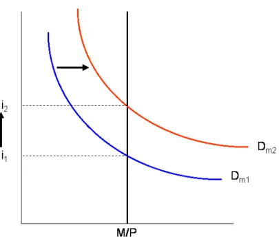
As such, bond prices are inversely proportional to yield or the interest rate. Consequently, when interest rates are low (near 2 percent in the case of Keynes’ analysis) or near zero in today’s environment, investors would believe that the rate can only go higher in the future. This would result in bond prices falling. Accordingly, investors would stay clear of bonds and hold their financial wealth in the form of money. Therefore, according to Keynes, the lower the current interest rate the lower the demand for bonds, and the greater the demand for money. Keynes referred to this as “liquidity preference” and a graphical depiction of it is provided in Figure 2 below.
Figure 2 Liquidity Preference
This graph shows that, at some low interest rate, the speculative demand for money, or as some analysts prefer the “interest-sensitive portion of demand for money”, becomes perfectly elastic with respect to the interest rate. At some low interest rate, all
Money Supply Function
investors would believe interest rates will only rise in the future (bond prices fall) and would therefore liquidate all bonds and hold all financial wealth in money.
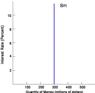
The Federal Reserve is responsible for determining the quantity of money supplied. Because the Fed can choose the quantity of money supplied, means that the money supply
function by itself is independent of the interest rate. Figure 3 illustrates the money supply function.12
Figure 3 The Money Supply Function
In the figure, the money supply is $300 million at all interest rate levels. If the Fed increases the money supply, the vertical money supply function shifts to the right. If the Fed decreases the money supply, the function shifts to the left.
Combining the money demand function with the money supply function shows how an increase in the money supply causes the interest rate to fall. See Figure 4 below.
12
Some economists depict the money supply function as upward sloping as opposed to vertical. Their rationale is that bank demand for excess reserves is negatively related to interest rates. Banks are more aggressive in lowering excess reserves (expanding loans and security holdings) as interest rate increases.
Figure 4 Money Supply Increases and Interest Rate Falls
As the money supply increases from Sm1 to Sm2, the equilibrium rate of interest falls
from i1 to i2. This is the cornerstone of Keynes model. “In Keynes view, if a change in the
money supply is to influence economic activity, it must do so via its impact on interest rates.”13 This is readily seen in Figure 5 below.
Figure 5 Keynesian Model
In the figure above, as the money supply increases from M1 to M2, the interest rate
declines from i1 to i2. However, note that when interest rates are low and the demand for money
is perfectly elastic, the increase in money supply has no effect on the interest rate. This is shown when M3 increases to M4; the interest rate remains constant at i3
↑
. In terms of MV = PQ, this means as M increases, V ↓ decreases proportionately. So, MV or aggregate demand, is unaffected by the expansion of the money supply when the money demand curve is perfectly elastic. The extra money supplied by the Federal Reserve is held in the form of speculative money; none of the money is spent. This is why Keynes’ believed that monetary policy is ineffective when interest rates are low, and the economy is caught in a “liquidity trap”.
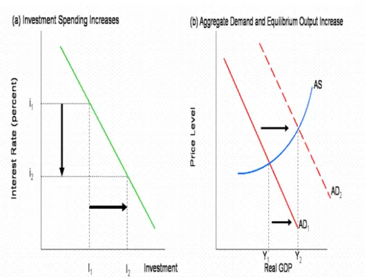
However, in normal times when the money demand curve is not perfectly elastic, lower interest rates stimulate spending and thus output. This is shown below in Figure 6.
Figure 6 Spending and Output Increases
In Figure 6(a) you can see the effect of lower interest rates on investment spending. As the interest rate falls from i1 to i2, investment increases from I1 to I2. When spending increases,
aggregate demand (AD) in figure 6(b) increases, shifting the AD curve rightward and increasing output from Y1 to Y2
Even though increasing the money supply normally reduces interest rates through the money demand equation, the interest rate can never go below zero percent. No one will lend money unless they get back, as a minimum, the amount they loaned. A negative interest rate would imply banks paying borrowers to take out loans. Therefore, once the Federal Reserve has increased the money supply to the point of lowering interest rates to zero, there would no longer be an impact on prices or output. In fact, in Keynes’ original work, The General Theory of Employment, Interest, and Money, it was suggested that a trap would occur at an interest rate of perhaps 2 percent, rather than at zero percent. Consequently, further increases in the money supply will be useless, and thus a “liquidity trap” will exist rendering monetary policy ineffective, as was previously shown in Figure 5.
.
A common approach for discussing a “liquidity trap” is through the use of the IS-LM model. The IS-LM model provides a framework for analyzing aggregate demand. It shows what
determines output for a given price level by analyzing the interaction between the goods and services market and the money market.14
IS-LM Derivation Method 1
As there are different meanings for “liquidity” and different meanings for “liquidity trap”, there are different approaches to developing the IS and LM curves in the IS-LM Model. The results are the same, which will become apparent as I show two derivations of the IS-LM curves for completeness and understanding. I will call the two different approaches to deriving the IS-LM curves simply, method 1 and method 2.
The following figure expresses that the quantity of money balances demanded, must equal the quantity of money balances supplied.
The LM Curve
Figure 7 Method 1 Derivation of LM Curve15
The speculative (or interest-sensitive portion of the) money demand function is shown in the 1st quadrant of Figure 7. The 3rd
14
N. Gregory Mankiw, Macroeconomics 5th ed., (Worth Publishers, New York, 2003) p. 531.
quadrant shows the transactions demand and precautionary
demand for money and is designated LT. It is a positive function of GDP. Quadrant 2 shows
different combinations of the existing money supply consisting of speculative holdings (LS) and
precautionary and transaction demand balances (LT
From Figure 7 it can be seen that the LM curve is made up from the demand for money (transaction, precautionary and speculative) and the money supply. It portrays the relationship between interest rates and GDP in equilibrium in the market for money.
). The LM curve is shown in quadrant 4 and is derived from the three other quadrants. The LM curve depicts all combinations of interest rates (i) and income levels (GDP) that are consistent with equilibrium in the market for money.
As an example, starting with the 1st quadrant, suppose the interest rate is 10 percent. The amount of money to satisfy the speculative demand for money is $50 billion. Quadrant 2 shows that, given the existing money supply of $150 billion, $100 billion is available to finance transactions and precautionary money demand. Quadrant 3 shows that, if LT
If the interest rate falls to 5 percent, quadrant 1 shows that speculative money demand increases. Given the existing money supply, fewer funds are available to satisfy transactions and precautionary motives. This, in turn, indicates that GDP must be lower in equilibrium (point B). Hence, the LM curve is an upward-sloping function of the interest rate.
is to be $100
billion, then GDP must be $500 billion. Therefore, a 10 percent interest rate in combination with $100 billion GDP will result in equilibrium. This is depicted as point A in quadrant 4 on the LM curve.
It can be seen that the LM curve depends upon the money supply and the demand for money. A change in the money supply or demand for money will result a change in the LM curve’s position. A change in the slopes of the speculative and/or precautionary demand for money will change the slope of the LM curve.
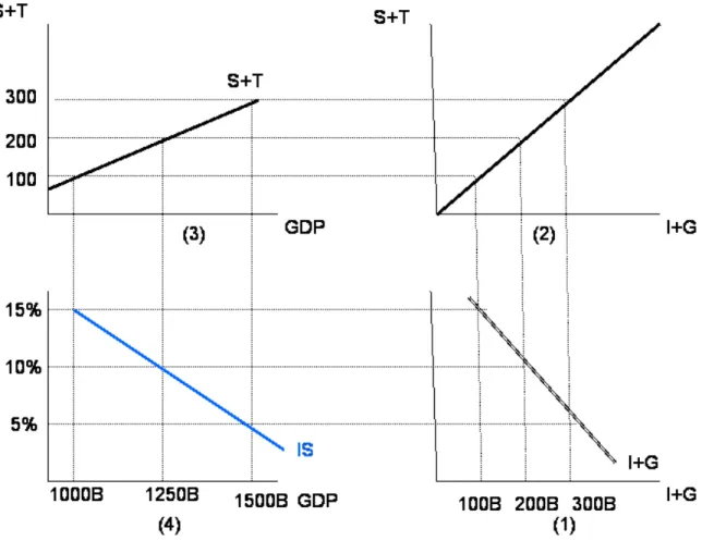
The IS Curve
The IS curve represents the various combinations of interest rates and levels of GDP that satisfies the state of equilibrium in the goods and services market. In a three-sector model, with no foreign trade, equilibrium occurs where S + T = I + G. That is, where leakages from income, in the form of Savings and Taxes (S+T), are offset by injections in spending by investments and government spending (I+G).
In quadrant (1) of Figure 8, I + G is a downward-sloping function of the interest rate. The lower the interest rate the greater the spending. To be in balance, the lower the interest rate, the higher S+T must be.
Figure 8 Method 1 Derivation of IS Curve16
The following example shows the derivation of the IS curve. Starting in quadrant (1), an interest rate of 10 percent implies spending (I+G) of $200B. If I+G is $200B, then to be in equilibrium, S+T must be $200B in quadrant (3). Subsequently quadrant (4) shows an equilibrium on the IS curve at an interest rate of 10 percent and a GDP of $1250B.
16 Ibid., p. 411.
The IS curve will shift rightward when any event shifts I+G rightward or S+T rightward. GDP in turn would expand. The IS curve will shift leftward when any event shifts I+G or S+T leftward. GDP would then contract.
General Equilibrium
It has been shown that there are an infinite number of possible combinations of interest rate and GDP levels that result in money market equilibrium. This is represented by a positive sloping LM curve. Likewise, it has been shown that there are an infinite number of possible combinations of interest rate and GDP levels that result in goods and services equilibrium. This is represented by a negative sloping IS curve. General equilibrium can be shown by the
intersection of the IS-LM curves. This is depicted in Figure 9.
Figure 9 Method 1 General Equilibrium
At the intersection of IS and LM the money market and the goods and services market are in equilibrium.
IS-LM Derivation Method 2
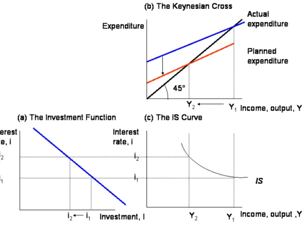
The IS Curve
As was previously mentioned in Method 1, in the IS-LM model, the IS (investment-saving) curve plots the relationship between interest rate and the level of output in the goods and services market. It is derived from the investment function, Figure 6(a), and the Keynesian Cross. The Keynesian Cross is a simple model of Keynes theory on national income. Keynes ideas, as outlined in his The General Theory of Employment, Interest, and Money (1936), proposed that an economy’s income was in the short run, determined largely by the desire to spend by households, firms, and the government. If there is idle capacity in the economy, the more people want to spend, and the more goods and services firms can sell. The more firms can sell, the more output they will choose to produce, and the more workers they will choose to hire. Thus, the problem during recessions and depressions, according to Keynes, was inadequate spending.17 The Keynesian Cross is a depiction of intended expenditure (the amount
households, firms, and government plan to spend on goods and services) versus the nation’s level of output and income. This is shown in Figure 10 below, with planned expenditures on the vertical axis and actual output and income on the horizontal axis.
Figure 10 Keynesian Cross
Combining the Investment Function, Figure 6(a), with the Keynesian Cross, Figure 10, one can derive the IS curve, as shown in Figure 11 below.
Figure 11 Method 2 Derivation of IS Curve
Figure 11(a) shows the investment function: an increase in the interest rate from i1 to i2
reduces planned investment from I1 to I2. Figure 11(b) shows the Keynesian Cross: a decrease
in planned investment from I1 to I2 shifts the planned expenditure function downward and
thereby reduces income from Y1 to Y2
The LM Curve
. Figure 11(c) shows the IS curve summarizing this relationship between interest rate and income: the higher the interest rate, the lower the level of output and income.
In the IS-LM model, the LM curve plots the relationship between the interest rate and the level of income or GDP (as in method 1), which arises in the market for money balances (money market). “In his classic work, “The General Theory”, Keynes offered his view of how the interest rate is determined in the short run. That explanation is called the theory of liquidity
preference, because it posits that the interest rate adjusts to balance the supply and demand for the economy’s most liquid asset-money. Just as the Keynesian cross is a building block for the IS curve, the theory of liquidity preference is the building block for the LM curve.”18 The theory of liquidity preference says that the supply and demand for money balances determines the interest rate. This is shown in Figure 12 below.
Figure 12 Liquidity Preference
The supply curve for money balances is vertical, because we assume the supply does not depend on the interest rate. The demand curve for money balances is downward sloping,
because higher interest rates raise the cost of holding money and thus lower the quantity demanded. The equilibrium interest rate is where the quantity of money balances demanded equals the quantity of money balances supplied.
Now that it has been shown how the interest rate is determined, the theory of liquidity preference can be used to show how the interest rate responds to changes in the money supply. This is shown below in Figure 13.
18 Ibid. p. 271.
Figure 13 Increase in the Money Supply Under Liquidity Preference
If the price level P is fixed, an increase in the money supply from M1 to M2 increases in
the supply of money balances (M/P). At i1, people are initially holding more money than they
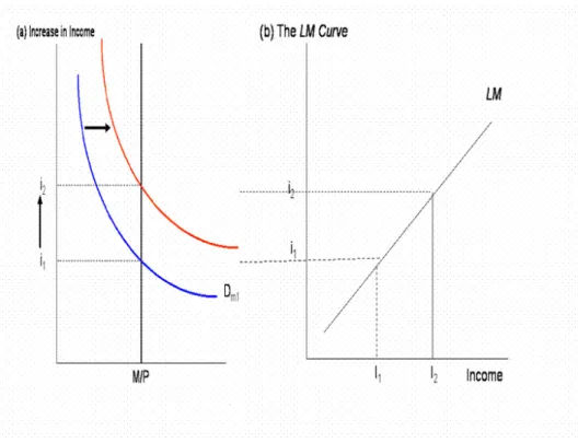
desire relative to bonds and other debt instruments. They use these excess money balances to buy bonds, driving up bond prices and reducing yields (the “interest rate”). The equilibrium rate therefore falls from i1 to i2,
Having shown how the theory of liquidity preference determines the interest rate, the LM curve can now be developed. The demand for money depends on income, as well as interest rates. Money demand varies directly with nominal income. As income increases, more
transactions are carried out and more money is required to finance those transactions. Therefore, the greater nominal income, the greater the demand for money. The increase in income shifts the demand for money curve upward, raising interest rates as shown below in Figure 14.
at which point the quantity of money demanded has caught up with the increased supply of money.
Figure 14 Increase in Income
With the supply of money balances unchanged, higher income leads to a higher interest rate.
The LM curve plots the relationship combinations of the levels of income and interest rate that would yield equilibrium in the market for money. The higher the level of income, the higher the demand for money, the higher the interest rate must be to produce equilibrium. This results in the LM curve sloping upward. This is shown below in Figure 15.
Figure 15 Method 2 Derivation of LM Curve
Figure 15(a) shows the effect an increase in income has on interest rates. Figure 15(b) shows the LM curve summarizing this relationship between interest rate (i) and income (I): the higher the level of income, the higher the interest rate must be, given the existing money supply. General Equilibrium
The IS-LM curves are shown together in Figure 16 below.
The IS-LM model joins the Keynesian Cross with the theory of liquidity preference. The IS curve shows all combinations of interest rate levels and income levels that satisfy equilibrium in the goods and services market. The LM curve shows all combinations of interest rate levels and income levels that satisfy equilibrium in the money market. The intersection of the IS-LM curves shows the interest rate and income that satisfy equilibrium in both markets. Note that the general equilibrium outcome is exactly the same for method 2 as it was for method 1.
Expansionary Monetary Policy
An expansionary monetary policy, depicted by an increase in the money supply is shown in Figure 17.
Figure 17 Expansionary Monetary Policy
An increase in the money supply raises money balances, shifts the LM curve rightward, lowers the interest rate, and raises income. Consequently, an increase in the money supply shifts the aggregate demand curve to the right, as shown in Figure 18 below.
Figure 18 Aggregate Demand
“Liquidity Trap”
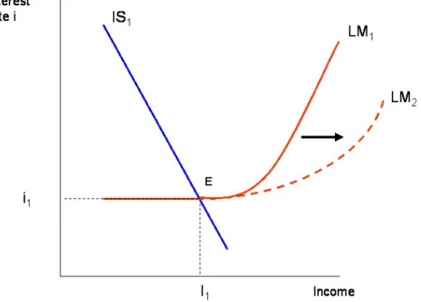
Based on the explanations thus far, it is now possible to show how a “liquidity trap” can be depicted in the IS-LM model. This is shown in Figure 19.
Figure 19 IS-LM Liquidity Trap
As the money supply M increases the LM curve shifts from LM1 to LM2. However, given
the position of the IS Curve and the shape of the LM Curve, the interest rate i1
“according to the IS-LM model, expansionary monetary policy works by reducing interest rates and stimulating investment spending. But if interest rates have already fallen almost to zero, then perhaps monetary policy is no longer effective. Nominal interest rates cannot fall below zero: rather than making a loan at a negative nominal interest rate, a person would simply hold cash. In this environment, expansionary policy raises the supply of money, making the public more liquid, but because interest rates can’t fall any further, the extra liquidity might not have any effect. Aggregate demand, production, and employment may be “trapped” at low levels.”
does not decrease and income does not increase, resulting in a “liquidity trap”. The IS-LM model is usually used to discuss a “liquidity trap” because
19
19 Ibid. p. 303.
Bank “Liquidity Trap”
Unlike a demand for money liquidity trap, a bank “liquidity trap” is a “potential situation in which bank demand for excess reserves is perfectly elastic with respect to the interest rate, rendering the central bank incapable of increasing the money supply”.20 In a bank liquidity trap, any additional excess reserves provided by the central bank are hoarded by banks, rather than being used to expand loans or security holdings. A graphical depiction of the relationship between interest rates and bank demand for excess reserves is displayed in Figure 20 below.
Figure 20 Bank Demand for Excess Reserves
If we combine the above graph depicting excess reserves with an increase in the bank reserves by the Federal Reserve, we can see that the increase in reserves has no effect on the money supply, again rendering monetary policy ineffective. This is shown in Figure 21 below.
Figure 21 Supply and Demand for Bank Excess Reserves
The reason why the bank demand curves for excess reserves become perfectly elastic as depicted above, is that at some low interest rate the risk associated with loaning the reserves and the transaction costs associated with using the reserves to buy government securities outweighs the meager expected rate of return (the interest rate).
Reasons Why Banks Hold More Money
The Federal Reserve controls the money supply through its ability to influence bank reserves and money creating power of banks. This can be expressed by a simple equation
B m
M = ⋅ , where M is the money supply, m is the money supply multiplier and B is the monetary base. The money supply multiplier is the ratio of the money supply to the monetary base. The monetary base consists of bank reserves and currency held by the public. The Federal Reserve normally manipulates the money supply through open market operations (the buying and selling of government bonds) that affect the monetary base. Banks are required to maintain a level of reserves (vault cash or deposit with the Federal Reserve). When the Federal Reserve increases the monetary base, the money supply increases by the multiplier, m times the increase in the base. Banks traditionally loan out almost all reserves in excess of the required amount,
because normally the opportunity cost of holding excess reserves is significant.21 However, when nominal interest rates are zero or close to zero, the opportunity cost of holding excess reserves becomes zero. Compounding this situation is the fact that bank precautionary hoarding may occur, along with tightened lending standards. Precautionary hoarding occurs when
financial intermediaries feel that they may need their own funds due to potential shocks to the economy, or if outside funding is expected to be difficult to obtain.22
How the Meaning of “Liquidity Trap” Has Changed Over Time.
Therefore, banks tend to hold excess reserves and the demand curve for excess reserves becomes highly elastic, at some low, positive interest rate, as is depicted above in Figure 21.
As quoted earlier, the phrase “liquidity trap” was coined by Sir Dennis Robertson, an English economist and colleague of John Maynard Keynes. Robertson used the phrase “liquidity trap” in critiquing Keynes’ idea of liquidity preference that Keynes used in his classical work The General Theory of Employment, Interest, and Money (1936). Robertson’s phrase “liquidity trap” was originally invented to illustrate the influence of a negatively sloped money demand on the saving-investment process, rather than a perfectly elastic demand for money, as the term is noted for today.23
Most of the “liquidity trap” literature associated with Keynes and another colleague of Keynes, Sir John R. Hicks, concerned the existence of a positive floor to the interest rate, not the zero or close to zero interest rate the liquidity trap is associated with today.24
21 The degree of significance has declined as the Federal Reserve has started paying some interest on
required bank reserves and excess bank reserves as of October, 2008. The interest rate paid on required reserve balances is determined by the Federal Reserve Board of Governors and is intended to remove part of the implicit tax that reserve requirements impose on depository institutions. The interest rate paid on excess reserve balances is also determined by the Board of Governors.Paying interest on excess balances is intended to establish a lower bound on the federal funds rate by lessening the incentive for institutions to trade balances in the fed funds market at rates much below the rate paid on excess balances. Paying interest on excess balances will permit the Federal Reserve to provide sufficient liquidity to support financial stability while conducting monetary policy in support of maximum employment and price stability goals.
It is Hicks and Alvin H. Hansen that are credited with developing the IS-LM model. It has been the model that has helped explain and espouse Keynesian economic policies.
22 Markus K. Bunnermeier, “Deciphering the Liquidity and Credit Crunch 2007-2008”, Journal of
Economic Perspectives, 23, No.1 (Winter 2009) 95.
23
Mauro Boianovsky, The IS-LM Model and the Liquidity Trap Concept: From Hicks to Krugman: History of Political Economy Conference on “The IS/LM Model: Its Rise, Fall and Strange Persistence”, Duke University, 25-27 April 2003, p. 15.
The ideas that underlie the “liquidity trap” were conceived in the Great Depression when short-term nominal interest rates were close to zero. As the memory of the Great Depression faded over time, and with inflation becoming the norm in the industrialized world following World War II, monetary policy, in a deflationary environment, largely remained the subject only of historical inquiries.25
Nevertheless, the liquidity trap received much more attention in the late 1990’s as the Japanese financial crisis unfolded along with the availability of new economic data. During the crisis, Japanese interest rates were essentially zero for most of the late 1990’s. The Bank of Japan more than doubled the monetary base, yet output remained stagnant.
With the Japanese crisis a modern view of a liquidity trap emerged. The modern view relies on economic models where aggregate demand depends on both current and expected future real interest rates, rather than simply the current rate, as with the traditional Keynesian economic models.
“The aggregate demand relationship that underlies the model is usually expressed by a consumption Euler equation, derived from the maximization problem of a
representative household. On the assumption that all output is consumed, that equation can be approximated as:
) ( 1 1 e t t t t t t t EY i E r Y = + −σ − π + −
where Yt is the deviation of output from the steady state, it is the short-term nominal
interest rate, πtis inflation, Et
e t
r
is an expectations operator and is an exogenous shock process (which can be due to host of factors). This equation says that the current demand depends on expectations of future output (because spending depends on expected future income) and the real interest rate which is the difference between the nominal interest rate and expected future inflation (because lower real interest rates make spending today relatively cheaper than future spending).”26
The importance of the equation is that it shows that monetary policy today might still be effective even if current interest rates are zero. Monetary policies would work through future expected inflation and thus future interest rates. The catch is that monetary policy must shape peoples expectations about future inflation.
25 Athanasios Orphanides, “Monetary Policy in Deflation: The Liquidity Trap in History and Practice”,
The North American Journal of Economics and Finance, vol. 15 (1) pp 101-124, March 2004.
26
Gauti, B. Eggertsson, “Liquidity Trap”, The New Palgrave Dictionary of Economics. Second Edition. Eds. Steven Nidurlauf and Lawrence E. Blume. Palgrave Macmillion, 2008.
Nobel economist Paul Krugman established in his May 1998 article, It’s baaack! Japan’s slump and the return of the liquidity trap that Japan’s monetary easing (near-zero interest rates and Bank of Japan’s balance sheet expansion by 50 percent per annum in 1998) failed because the Bank of Japan was unable to change the public’s expectations about future inflation. When nominal interest rates are near zero, expected inflation needs to be positive to keep ex ante real interest rates sufficiently low and thus impact private spending and aggregate demand. When, the public expects the central bank to maintain price stability, as the Japanese populace did with the Bank of Japan, then inflation expectations remain very low resulting in ex ante real interest rates being too high to spur spending by the public. This failure to initiate an increase in aggregate demand renders monetary policy ineffective.
Accordingly, the only way out of a liquidity trap is to raise inflationary expectations. This is possible by government increasing deficit spending with fiscal policy or with
“irresponsible monetary policy” – that is, convincing the public that monetary expansion is not merely temporary and that the central bank will not reverse its policy of monetary expansion when prices begin to rise.27
Theory Review
Normally, the Federal Reserve can stimulate the economy by increasing the monetary base and lowering interest rates. Typically these actions, increase borrowing, investment, and aggregate spending. However, when interest rates are near zero, the Federal Reserve can no longer lower interest rates to stimulate the economy. The Federal Reserve can increase the monetary base. This money must find its way into the economy, which is normally
accomplished through the banks. However, the banks are unwilling to lend, so the newly created liquidity is trapped behind unwilling bank lenders, thus forming the liquidity trap.28
27
Paul Krugman, “It’s baaack! Japan’s slump and the return of the liquidity trap. Brookings Papers on Economic Activity 1998 (2). 137-187.
Therefore, when nominal interest rates are close to zero, the opportunity cost of holding money becomes negligible and banks, firms and individuals hold more money than they need for transaction purposes. Traditional monetary policy becomes ineffective in stimulating the economy because the money creation process does not function. In turn, the liquidity trap brings about inability to combat deflation, i.e. a continuous decline in prices. When deflation is persistent, even if
combined with an extremely low interest rate, a floor on real interest rates creates a vicious cycle of output stagnation and further expectations of deflation that perpetuates high real interest rates and continuing economic stagnation.29
29
Hiro Ito, “Liquidity Trap”, The Princeton Encyclopedia of the World Economy, Eds. Kenneth Reinert and Ramkishen Rajas, Princeton University Press, December 2008.
CHAPTER 2 - Is There Evidence of Liquidity Trap?
I will now review recent data to shed light on the question whether the United States is in a “liquidity trap”.
Demand for Money “Liquidity Trap”
Based on the presented explanations, the first requirement for a “liquidity trap” is that short term nominal interest rates be near zero. The following data regarding the federal funds rate show that is in fact the case today.
Figure 22 Federal Funds Rate
In its effort to ward off a recession, the Federal Reserve started reducing its federal funds rate in August 2007. It continued reducing the interest rate until it reached it’s historic lows on December 16, 2008 of a target rate between zero and quarter percentage point. That target, of between zero and a quarter percentage point, has continued throughout 2009 to date (December
2009). The Federal Reserve also reiterated, at its Federal Open Market Committee (FOMC) meeting in November of 2009 that it expects to keep the target rate between zero and a quarter percentage point for the foreseeable future.
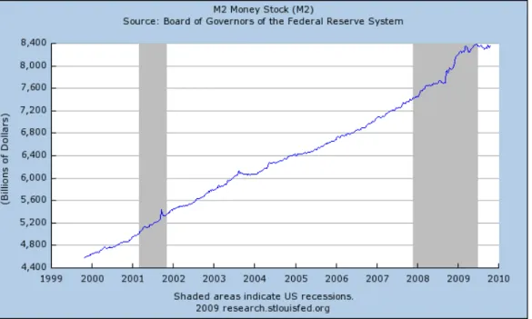
The second requirement for a money demand liquidity trap is that when the Federal Reserve increases the money supply, it has no effect on output or prices. The following graph shows that the money supply (M2) has increased, indeed, at an above-trend pace since the beginning of 2008. M1 has also increased at an above-trend rate.
Figure 23 M2 Money Supply
The M2 monetary aggregate increased at a 10 percent annual rate during the second half of 2008 and 8.5 percent for the year as a whole.30
30
Board of Governors of the Federal Reserve System, “part 2, Recent Financial and Economic
Developments” Monetary Policy Report to Congress, February 2009,. p. 25-26. M2 consists of (1) currency outside the U.S. Treasury, Federal Reserve Banks, and the vaults of depository institutions; (2) traveler's checks of nonbank issuers; (3) demand deposits at commercial banks (excluding those amounts held by depository institutions, the U.S. government, and foreign banks and official institutions) less cash items in the process of collection and Federal Reserve float; (4) other checkable deposits (negotiable order of withdrawal, or NOW, accounts and automatic transfer service accounts at depository institutions, credit union share draft accounts, and demand deposits at thrift institutions); (5) savings deposits (including money market deposit accounts); (6) small-denomination time deposits (time deposits in amounts of less than $100,000) less individual retirement account (IRA) and Keogh balances at depository institutions; and (7) balances in retail money market mutual funds less IRA and Keogh balances at money market mutual funds.
the Congress, the Federal Reserve states that “the M2 monetary aggregate expanded at an annual rate of 7 ¾ percent during the first half of 2009.”31
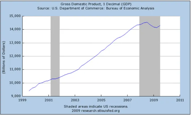
Figure 24 Nominal GDP
Figure 24 above shows that nominal GDP in the United States declined slightly in the third quarter of 2008 and then decreased at an annualized rate of 6.3 percent in the 4th quarter. The decline continued at a 6.4 percent annual rate in the 1st quarter of 2009 and at an annual rate of 1% in the second quarter of 2009. 32 This decrease occurred despite the sharp increase in the money supply and decrease in short term nominal interest rates. However, nominal GDP did increase at an annual rate of 2.8 percent in the third quarter of 2009. 33 This increase in nominal GDP reflects upturns in personal consumption expenditures, exports, private inventory
investment, federal government spending and residential fixed investment.
31 Board of Governors of the Federal Reserve System, “part 2, Recent Financial and Economic
Developments” Monetary Policy Report to Congress, July 21, 2009, p. 25.
32 Bureau of Economic Analysis, “News Release” regarding National Income and Product Account Gross
Domestic Product: Second Quarter 2009 (Advance Estimate), July 31, 2009.
33
Bureau of Economic Analysis, “News Release” regarding National Income and Product Account Gross Domestic Product: Third Quarter 2009 (Advance Estimate), October 29, 2009.
Table 1 Equation of Exchange Variables FISCALYEAR GDP (IN BILLIONS) M2 (IN BILLIONS) VELOCITY (GDP/M2) %Δ M2 %ΔV 2006:1 13183.5 6647.9 1.983 --- --- 2006:2 13347.8 6743.5 1.979 1.43 -0.20 2006:3 13452.9 6803.6 1.977 0.89 -0.10 2006:4 13611.5 6879.1 1.979 1.11 0.10 2007:1 13795.6 6994.0 1.972 1.67 -0.35 2007:2 13997.2 7096.3 1.972 1.46 0.00 2007:3 14179.9 7198.8 1.970 1.44 -0.01 2007:4 14337.9 7298.4 1.965 1.38 -0.25 2008:1 14373.9 7405.3 1.941 1.46 -1.22 2008:2 14497.8 7560.2 1.918 2.09 -1.18 2008:3 14546.7 7666.5 1.897 1.40 -1.09 2008:4 14347.3 7744.1 1.853 1.01 -1.75 2009:1 14178.0 8020.0 1.768 3.56 -4.59 2009:2 14151.2 8278.2 1.709 3.21 -3.34 2009:3 14301.5 8360.2 1.711 0.99 0.12
Although the equation of exchange is simply an identity, it is instructive to review the behavior of the variables in this equation. The above table created from FRED (Federal Reserve Economic Data) displays the equation of exchange variables from the first quarter of 2006 (approximately a year before the start of the current recession) until the third quarter of 2009 (the latest data available). M2 is the quarterly average of the monthly data reported in FRED.34
34
M2 includes a broader set of financial assets held principally by households. M2 consists of M1 plus: (1) savings deposits (which include money market deposit accounts, or MMDAs); (2) small-denomination time deposits (time deposits in amounts of less than $100,000); and (3) balances in retail money market mutual funds (MMMFs). Seasonally adjusted M2 is computed by summing savings deposits, small-denomination time deposits, and retail MMMFs, each seasonally adjusted separately, and adding this result to seasonally adjusted M1.
The table shows that, as the Federal Reserve increased the money supply, the country’s nominal output (GDP) increased from 2006:1 until the 2008:3. Subsequently, nominal GDP started to fall and continued to decline up until the third quarter of 2009, when it rose. In the context of the equation of exchange, the proximate cause of this decline in GDP is the decline in velocity. Velocity has decreased persistently throughout the range of data (until the third quarter 2009), slowly at first, and then considerably faster starting in 2008:1. There are two particular items of note. First, from 2008:3 through 2009:2, the percent decline of velocity was greater than the
percent increase in the money supply (M2). This explains the decline in nominal GDP. Additionally, the drops in velocity are rates per quarter. This means that the annual rate of decline in velocity in 2009:1 was 18.4 percent per year! Velocity decreased as households and firms increased money holdings relative to expenditures.
A graphical depiction of the GDP and Velocity columns in the above table are provided in Figures 25 and 26 respectively. In the three years ending in 2009:2, M2 velocity declined about 14 percent Figure 25 Nominal GDP 12500 13000 13500 14000 14500 15000 2006:Q1 2006:Q2 2006:Q3 2006:Q4 2007:Q1 2007:Q2 2007:Q3 2007:Q4 2008:Q1 2008:Q2 2008:Q3 2008:Q4 2009:Q1 2009:Q2 2009:Q3
Figure 26 Velocity (GDP/M2) 1.55 1.6 1.65 1.7 1.75 1.8 1.85 1.9 1.95 2 2.05 2006:Q1 2006:Q2 2006:Q3 2006:Q4 2007:Q1 2007:Q2 2007:Q3 2007:Q4 2008:Q1 2008:Q2 2008:Q3 2008:Q4 2009:Q1 2009:Q2 2009:Q3
The following graph also shows that despite an increase in the money supply and a decrease in interest rates, prices at the producer level have generally fallen. The index declined from a high of 205.5 in July 2008 to 168.1 in March 2009, showing a fall in prices of
approximately 18 percent in this 8-month period. Prices have risen and fallen slightly since March 2009 with a measure of 174.6 as of September 2009, resulting in an overall decline of nearly 15 percent since the high of July 2008.
Figure 27 Producer Price Index
These graphs suggest that monetary policy has been ineffective and is consistent with the hypothesis that a “liquidity trap” exists based on the typical understanding of the meaning “liquidity trap”. Increases in the money stock engineered by the Federal Reserve have not resulted in an increase in aggregate expenditures.
In chapter 1, it was stated that the slope of the demand for money curve plays an important role in macroeconomics because the slope determines whether monetary policy or fiscal policy exerts more influence on aggregate demand. A graph depicting the recent
relationship between the 3-Month Treasury bill rate and money balances using the same M2 data as in Table 1 is shown below.
Figure 28 Money and Interest Rates 2006:1-2009:3
Supporters of Keynesian theory believe that fiscal policy plays a greater role than monetary policy in influencing aggregate demand in a low interest rate environment. They believe that the quantity of money demanded is sensitive to the interest rate and that the money demand curve shifts as it reacts to various economic events, thus making velocity volatile. Those that believe monetary policy has a greater influence in shaping the aggregate demand curve, otherwise known as monetarists, believe that the demand for money curve is nearly vertical and quite stable. The above graph may lead one to believe that, in this financial crisis, the monetarists are correct. One may believe that monetary policy has had a greater influence in shaping the aggregate demand curve since the relationship curve shown above is nearly vertical. However, the demand for money depends also on other factors such as income and economic uncertainty. Consequently, it would be useful to analyze the interest elasticity of money demand to help determine if a “liquidity trap” truly exists. As referred to in Chapter 1, the interest
elasticity of money demand plays an important role in macroeconomics. Keynesians believe that the interest elasticity of demand for money is relatively high (-0.5 to -1.0), while monetarists
believe that the elasticity is quite low (-0.1 to -0.3)35. According to David E. W. Laidler “If the liquidity trap hypothesis is true, it must be the case that the interest elasticity of demand for money becomes greater as the rate of interest falls…” 36
∞ → ∆ ∆ i DM 0 0 0 0
In a liquidity trap the interest elasticity of demand goes to infinity at some very low interest rate, as the percent change in demand for money is divided by the percent change in interest rate, as shown by the following formula.
Of note however, is Laidler’s follow on statement regarding this relationship. He states that “there appears to be little evidence that this is in fact the case.”37
Regression Analysis to Investigate Interest Elasticity of Money Demand
This statement not withstanding, regression analysis can be used to estimate the interest elasticity of demand for money, which in turn, will help determine the existence of a liquidity trap.
Regression Procedure
To determine the existence of a traditional demand for money liquidity trap, different regression iterations of the following equation were run.
(
GDP)
delta(
Risk)
gamma(
InterestRate)
beta alpha P M ln ln ln ln = + + + P M
was determined by using monthly data for both M1 and M2. Then, each was divided by the Consumer Price Index (CPI). CPI is a representative variable for Price (P). M2 was used to be consistent with Table 1 and Figure 28. However, M2 includes several highly liquid financial assets, such as savings deposits and money market mutual fund shares that pay interest. It is also a broader measure of money that is used when one wants to emphasize the store-of-value function of money. Consequently, regressions were also run using M1, a measure
35 Lloyd B. Thomas, Jr., Money, Banking, and Economic Activity, third edition. Prentice-Hall Inc.1986, p.
343.
36
David E. W. Laidler, Demand for Money Theories, Evidence& Problems, fourth edition. HarperCollins College Publishers. 1993, p. 150.
that includes currency, demand deposits and other checkable deposits that pay little to no interest and emphasizes the medium exchange function of money.
Since GDP data are reported in FRED on a quarterly basis, monthly GDP data were estimated by using interpolation. The interest rate used was the 90-day Treasury bill yield. Risk, a gauge of economic uncertainty, was measured by using the difference between Moody’s Aaa corporate bond yield and Moody’s Baa corporate bond yield, as reported in FRED. A priori, one expects the signs on beta, delta, and gamma to be positive, positive, and negative, respectively.
Periods of different interest rates were used to observe how gamma changed when interest rates were relatively low, as compared to times when interest rates were higher. Data were chosen that went back fifteen years to 1994. Regressions were run using data through April 2009. April of 2009 was the latest date that data were available for all variables, since GDP data, at the time, only existed for the first two quarters of 2009.
The log-linear model with equation lnY =β1+β2lnX was used as the functional form. This is also known as the double-log form and is the most common functional form. In this form, the natural log of Y is the dependent variable and natural log of X is the independent variable. Generally, this functional form is used when slopes are not constant. This is the case for interest elasticity of demand for money and thus the reason for using this functional form. Natural logs also make it easier to determine impacts in percentage terms. “If you run a double-log regression, the meaning of a slope coefficient is the percentage change in the dependent variable caused by a one percentage point increase in the independent variable, holding the other independent
variables in the equation constant. It’s because of this percentage change property that the slope coefficients in a double-log equation are elasticities.”38
Regression Results
Regression results are reported in the following table.
38
A. H. Studenmund, Using Econometrics, A Practical Guide, fifth edition, Pearson Education Inc. 1996, p. 211.
Table 2 Estimation of Money Demand Model (January 1994- April 2009)
Note: The numbers in parentheses are t-statistics calculated by using the Newey-West method. Regression Analysis
The most pertinent finding in the above table pertains to gamma. Gamma is an estimate of the interest elasticity of demand for real money balances (M/P). In a pure liquidity trap this would be negative infinity. Otherwise, as previously detailed by David Laidler, the interest elasticity of demand or gamma should increase (in absolute terms) as interest rates fall. This occurs for some of the regression iterations. For example, when comparing gamma for M1/P when interest rates were greater than 1 percent, with interest rates when they fell to less than or equal to 1 percent, the regression iteration
te InterestRa gamma alpha P M ln 1 ln = +
ln M1/P = alpha + beta ln GDP + delta ln Risk + gamma ln Interest Rate
alpha ln GDP ln Baa-Aaa ln Interest
Rate # obs R Interest Rates < 1% 2 1.945 (390.87) -.028 (-9.48) 18 0.725 3.007 (3.62) -.113 (-1.27) -.038 (-4.28) 18 0.769 1.796 (2.49) .016 (0.21) -.033 (-3.03) -.043 (-4.16) 18 0.804 Interest Rates > 1% 1.908 (221.84) -.009 (1.36) 166 0.007 3.225 (18.14) -.138 (-7.40) -.017 (-2.59) 166 0.257 2.817 (15.27) -.093 (-4.76) -.089 (-5.80) -.041 (-5.53) 166 0.322
ln M2/P = alpha + beta ln GDP + delta ln Risk + gamma ln Interest Rate Interest Rates < 1% 3.502 (369.38) -.070 (-4.34) 18 0.764 -1.785 (-1.72) .564 (5.07) -.020 (-1.69) 18 0.952 -.400 (-0.45) .416 (4.33) .038 (3.33) -.014 (-1.15) 18 0.960 Interest Rates > 1% 3.570 (227.37) -.168 (-12.30) 166 0.311 -2.150 (-30.61) .603 (79.87) -0.48 (-15.56) 166 0.986 -2.158 (-30.90) .604 (81.62) -.001 (-0.20) -.048 (-16.84) 166 0.986
ln M1/P = alpha + beta ln GDP + delta ln Risk + gamma ln Interest Rate Interest Rates < 2% 1.926 (443.85) -.045 (-7.07) 50 0.600 2.956 (10.46) -.109 (-3.64) -.053 (-6.69) 50 0.658 2.374 (9.47) -.046 (-1.72) -0.64 (-6.23) -.071 (-7.48) 50 0.796 Interest Rates > 2% 1.952 (58.49) -.018 (-0.83) 134 0.005 3.479 (17.54) -.156 (-7.87) -.078 (-3.77) 134 0.311 3.273 (13.21) -.134 (-5.45) -.038(-1.46) -0.081 (-.416) 134 0.318
ln M2/P = alpha + beta ln GDP + delta ln Risk + gamma ln Interest Rate Interest Rates < 2% 3.506 (516.98) -0.67 (-6.01) 50 0.572 -.540 (-3.51) .431 (26.22) -.036 (-5.53) 50 0.966 -.521 (-3.77) .428 (29.11) .002 (0.34) -0.035 (-5.11) 50 0.966 Interest Rates > 2% 3.774 (67.94) -.299 (-8.18) 134 0.229 -2.210 (-29.54) .612 (81.99) -.063 (-9.62) 134 0.989 -2.118 (-22.41) .603 (65.02) .017 (1.64) -.062 (-9.40) 134 0.990
shows that gamma increased (in absolute terms) for all three iterations from -.009 to -.028, from -.017 to -.038 and from -.041 to -.043 respectively. These low interest elasticities (fairly close to zero) do not confirm the existence of a liquidity trap. However, when comparing gamma for M1/P when interest rates were greater than 2 percent, with interest rates when they fell to less than or equal to 2 percent, there is only one iteration that increased and that was from -.018 to -.045. This is not to be unexpected, as there is less likelihood of a liquidity trap at higher interest rates.
Note that the coefficients on the ln GDP variable exhibit the expected sign in the M2/P regressions and exhibit very high t-statistics. These coefficients range in magnitude from roughly 0.40 to 0.60, indicating that M2 is a normal good, confirming economies of scale in money balances. As GDP rises over time, demand for M2 rises more slowly. However, in the M1/P regressions, the signs on the estimated ln GDP coefficients are uniformly negative and often highly significant statistically.
This result is likely picking up the action taken by the Federal Reserve to pump liquidity into financial markets since the beginning of the financial crisis. From January 2008 to
September 2009, M1 increased more than 19 percent. This is most likely the reason M1/P regressions are exhibiting the wrong sign on the GDP and risk variables. M2/P regression results are better. M2 has only grown by 11 percent over the same time period. This is probably because M2 has not been impacted as much by the Federal Reserve actions.
The regressions indicate that the measure for risk, ln(Baa –Aaa) is statistically
insignificant in the M2/P regressions, and exhibits the wrong sign in the M1/P regressions (and is sometimes statistically significant). This may be because the risk variable (Baa-Aaa) and the loss of confidence that was occurring in the economy were not picking up the shifts that were occurring in the money demand function. It is extremely difficult to disentangle the effect of very low interest rates from other forces causing increases in money demand here such as safe haven forces, as the stock market crashed (Dow Jones Industrial Averages fell from a high of nearly 14,000 in October of 2007 to a low of nearly 6600 the second week of March 2009) .
Bank “Liquidity Trap”
What about a bank “liquidity trap”? Previously, it was stated that a bank “liquidity trap” is a potential situation in which bank demand for excess reserves is perfectly elastic with respect
to the interest rate, rendering the central bank incapable of increasing the money supply. In this situation, all additional reserves injected into the banks by the Federal Reserve are simply held by the banks, rather than being used to extend credit. The following graphs show this. Figure 29 shows total bank reserves and figure 30 shows the excess reserves held by banks.
Figure 29 Total Bank Reserves
Clearly, banks started to rigorously hold excess reserves midway through 2008. They continue to do so as the nominal short-term interest rates have remained near zero and as the opportunity cost of holding excess reserves is extremely low.
Banks also build up excess reserves if they cut back on their lending through a tightening of standards or for precautionary reasons. The following graph shows that the amount of loans that banks have made has declined, even as excess reserves increased. In fact, the decline started in earnest about the time the Federal Reserve lowered its interest rate target to between a quarter and zero percent. In its February 2009 monetary report to Congress, the Board of Governors reported a decreased demand for credit in response to slowing business activity along with a tightening of lending standards.39 Additionally, the Senior Loan Officer Opinion Survey conducted in April 2009 “indicated that large fractions of banks continued to tighten lending standards and terms on loans to businesses and households over the preceding three months”.40
Figure 31 Amounts of Bank Loans
39 Board of Governors of the Fede