http://wrap.warwick.ac.uk/
Original citation:
Ortner, Christoph, Shapeev, Alexander V. and Zhang, Lei. (2014) (In-)stability and stabilisation of QNL-Type atomistic-to-continuum coupling methods. Multiscale Modeling & Simulation: a SIAM Interdisciplinary Journal . ISSN 1540-3459 (Accepted)
Permanent WRAP url:
http://wrap.warwick.ac.uk/60737
Copyright and reuse:
The Warwick Research Archive Portal (WRAP) makes this work of researchers of the University of Warwick available open access under the following conditions. Copyright © and all moral rights to the version of the paper presented here belong to the individual author(s) and/or other copyright owners. To the extent reasonable and practicable the material made available in WRAP has been checked for eligibility before being made available.
Copies of full items can be used for personal research or study, educational, or not-for-profit purposes without prior permission or charge. Provided that the authors, title and full bibliographic details are credited, a hyperlink and/or URL is given for the original metadata page and the content is not changed in any way.
Publisher’s statement: © SIAM
http://www.siam.org/journals/mms.php
A note on versions:
The version presented here may differ from the published version or, version of record, if you wish to cite this item you are advised to consult the publisher’s version. Please see the ‘permanent WRAP url’ above for details on accessing the published version and note that access may require a subscription.
ATOMISTIC-TO-CONTINUUM COUPLING METHODS
C. ORTNER, A. V. SHAPEEV, AND L. ZHANG
Abstract. We study the stability of ghost force-free energy-based atomistic-to-continuum coupling
methods. In 1D we essentially complete the theory by introducing a universally stable a/c coupling as well as a stabilisation mechanism for unstable coupling schemes.
We then present a comprehensive study of a two-dimensional scalar planar interface setting, as a step towards a general 2D/3D vectorial analysis. Our results point out various new challenges. For example, we find that none of the ghost force-free methods known to us are universally stable (i.e., stable under general interaction and general loads). We then explore to what extent our 1D stabilisation mechanism can be extended.
1. Introduction
Atomistic-to-continuum (a/c) coupling schemes are a class of computational multiscale methods for the efficient simulation of crystalline solids in the presence of defects. Different variants have been among the tools of computional materials science for many decades [18, 9, 19]. More recently, a numerical analysis theory of a/c coupling has emerged; we refer to [17] for an introduction, a summary of the state of the art, and extensive references.
While theconsistencytheory of a/c coupling methods has a solid foundation [21, 23], understanding their stability properties essentially remains an outstanding open problem. The main difficulty is that the a/c model interface, even if treated consistently, can generate new eigenmodes present in neither the atomistic nor continuum model, which can render a/c coupling methods unstable. Indeed, we emphasize that we are not only concerned with questions of analysis, but also with the construction of stable schemes.
In one dimension, an essentially complete survey of stability is presented in the review article [17], which is partially based on the results of the present article. In dimension greater than one very little is known. A universal stability result has been proven in [15], but for a coupling scheme that requires a macroscopically thick interface region. Some recent progress on getting sharp bounds on the required blending width for force-based a/c coupling [11, 12] remains incomplete and partially based on numerical evidence. For a sharp interface force-based coupling scheme more comprehensive analytical results are presented in [16], but even these are restricted to flat a/c interfaces and are dependent upon conditions that cannot be readily checked analytically.
In the present work we focus on the stability of a particular class of conservative a/c schemes, generally called quasinonlocal (QNL) type coupling schemes. In one dimension we present examples of stability and instability (§3), construct a new “universally stable” scheme (§4), and further show how unstable QNL schemes can be stabilised (§5).
We then consider a two-dimensional model problem, for which our results are more limited, in that we need to make much more stringent assumptions on the deformation and interaction potential than in 1D. Within these assumptions, we show that there is a source of instability in 2D interfaces, which was not present in the 1D setting (§7.1). Moreover, we show that this instability is universal. It is not only present in specific instances of QNL type a/c couplings, but in a fairly wide class of generalized geometric reconstruction methods [25] (§7.2) which cover most of the existing methods. This new source of instability is more severe than the instabilities observed in 1D and cannot be “easily” stabilised. To be precise, we show that stabilising QNL type schemes in 2D severely affects their consistency when the system approaches a bifurcation point (§7.4).
Date: January 25, 2014.
2000Mathematics Subject Classification. 65Q99, 74S30, 65N12, 70C20.
Key words and phrases. atomistic-to-continuum coupling, quasicontinuum, stability.
CO and LZ were supported by the EPSRC grant EP/H003096 “Analysis of atomistic-to-continuum coupling methods”. AS was supported by AFOSR Award FA9550-12-1-0187.
2. A General 1D QNL Formulation
2.1. Notation for lattice functions. For a lattice function v :Z → R and ρ ∈ Z\ {0}, we define the finite difference operators
Dρv(ξ) :=v(ξ+ρ)−v(ξ).
For some finite interaction stencil R = {±1, . . . ,±rcut}, where rcut ∈N is a fixed cut-off radius, we define
Dv(ξ) := Dρv(ξ)
ρ∈R. The space of compact displacements is defined by
W0 :=
u:Z→Rsupp(u) is bounded .
Each lattice function v :Z → R is identified with its canonical continuous piecewise affine inter-polant. In particular, we define the gradients ∇v(x) :=v(ξ)−v(ξ−1) forx∈(ξ−1, ξ).
IfH :W0 →W0∗ is a linear operator (or,hH·,·ia bilinear form onW0), then we define the associated
stability constant
γ(H) := inf u∈W0 k∇ukL2=1
hHu, ui.
We say that H is stable if γ(H)>0.
2.2. Many-body interactions for an infinite chain. We consider finite-range many-body inter-actions of deformed configurations of the infinite chain Z. Let V ∈ C2(RR) be the many-body site energy potential with partial derivatives
Vρ(g) :=
∂V(g)
∂gρ
and Vρς(g) :=
∂2V(g)
∂gρ∂gς
forg= (gρ)ρ∈R∈RR.
We assume thatV is invariant under reflections of the local configuration, that is,
V (gρ)ρ∈R =V (−g−ρ)ρ∈R. (2.1)
Immediate consequences of (2.1) are the symmetries
V−ρ(FR) =−Vρ(FR) and V−ρ,−ς(FR) =Vρς(FR) ∀ρ, ς∈ R,F>0. (2.2)
A macroscopic strainFand a displacementu∈W0induce a deformed configurationy(ξ) =Fξ+u(ξ),
ξ∈Z. To such a configuration we assign the energy difference
Ea(y) :=X ξ∈Z
V(Dy(ξ))−V(FR). (2.3)
Since the lattice sum is finite, this expression is well-defined. The first and second variations with respect tou (in the sense of Gateaux derivatives) are also well-defined and are given by
hδEa(y), vi:=X ξ∈Z
X
ρ∈R
Vρ(Dy(ξ))·Dρv(ξ), and
hδ2Ea(y)v, vi:=X ξ∈Z
X
ρ,ς∈R
Vρς(Dy(ξ))·Dρv(ξ)Dςv(ξ), forv∈W0.
We are particularly interested in the second variation evaluated at the homogeneous deformation
y=Fx (where (Fx)(ξ) :=Fξ),
hHFav, vi:=hδ2Ea(Fx)v, vi=X ξ∈Z
X
ρ,ς∈R
Vρς ·Dρv(ξ)Dςv(ξ), (2.4)
where, here and throughout most of this work, we are suppressing the dependence ofVρς onFRwhen it is clear from the context that we meanVρς(FR).
2.3. A general QNL formulation. The QNL approximation of Ea [28] transitions between the
atomistic model and a continuum model by introducing modified site potential at the a/c interface. To simplify our analysis we focus on a single a/c interface. Let Z− :={−∞, . . . ,0} be the atomistic region and R+ := (0,∞) the continuum region. In the atomistic region, we employ modified site
energies ˜Vξ ∈ C2(RR), ξ ≤ 0, while, in the continuum region we employ the Cauchy–Born strain energy density [1, 10, 8, 24],
W(G) :=V(GR).
The QNL a/c coupling energy functional is then given by
Eac(y) :=
0
X
ξ=−∞ ˜
Vξ(Dy(ξ))−V(FR)
+
Z ∞
1/2
W(∇y)−W(F)dx, (2.5)
for all deformations y=Fx+u, u∈W0.
We shall assume throughout that the modified site energies satisfy the following conditions: there existsξ0 ∈Z− such that
˜
Vξ,ρ(Dy(ξ)) = 0 whenever ξ+ρ >1, (2.6) ˜
Vξ(Dy) =V(Dy) forξ≤ξ0, (2.7)
δEac(Fx) = 0 ∀F>0. (2.8)
Condition (2.6) states that atoms do not interact with the continuum region, except for the interface atom at ξ = 0. Condition (2.7) states that the transition region is bounded. Condition (2.8) is the force-consistency condition (absence of “ghost forces”), which ensures first-order consistency of the QNL approximation [21].
As in the case of the atomistic model, Eac is well-defined and has variations in the sense of
Gateaux derivatives. The second variation, evaluated at the homogeneous deformation y = Fx,
HFac=δ2Eac(Fx), is given by
hHac
F u, ui=
0
X
ξ=−∞ X
ρ,ς∈R ˜
Vξ,ρς·Dρu(ξ)Dςu(ξ) +W00(F)
Z ∞
1/2
|∇u|2dx. (2.9)
2.3.1. Error in critical strains. We shall be interested in understanding the regimes of strains F for which HFa and HFac are stable. To explain why this is relevant in practical simulations, consider the following description of a quasi-static loading scenario (adapted from [5]):
(i) F(t)∈C([t0, t∗]) is a given path in deformation space, wheret∗is a critical load, and constants c0, c1 >0, such that
c0(t∗−t)≤γ(HFa(t))≤c1(t∗−t) fort0≤t≤t∗.
At the critical load t∗ (e.g., a bifurcation) an instability occurs, which typically indicates the onset of defect nucleation of defect motion (“critical event”).
(ii) Suppose now that QNL is initially stable but has a reduced stability region: γ(HFqnl(t
0))>0 but γ(HFqnl(t∗))<0. Then, there exists a reduced critical load tqnl∗ < t∗ such that γ(Hqnl
F(tqnl∗ )) = 0.
In such a situation we first of all predict an incorrect critical load, i.e., incorrect magnitude applied forces under which the critical event occurs. Moreover, since the event may occur in a different region of deformation space, it is even possible that a qualitatively different event is observed (e.g., a different type of defect is nucleated).
2.3.2. Preliminary estimates. We can immediately make the following generic observation.
Proposition 2.1. γ(HFac)≤γ(HFa) for all F>0.
Remark 2.2. If the atomistic region is finite, then we would obtain thatγac(G)≤γa(F) + err, where err decreases with increasing atomistic region size. See [10] for results along these lines.
Proof. Letε >0 and let u∈W0 such thatk∇ukL2 = 1 andhHau, ui ≤γa(F) +ε. Upon shiftingu by v(ξ) =u(ξ+η) for η sufficiently large, we can assume without loss of generality that u(ξ) = 0 for all
ξ≥ξ0−rcut−1. Therefore, we obtain
Since εwas arbitary, the result follows.
Proposition 2.1 ensures that, if a latticeFZis unstable in the atomistic model, then it must also be unstable in the a/c coupling model. The converse question, whether stability of HFa implies stability of HFac is more difficult to answer in general. This question was first raised in [5] for 1D second-neighbour Lennard-Jones type pair interactions, where this implication holds. Further investigations in this direction can be found in [6, 14, 13]. In the present work we aim to present a more complete picture for the case of general range many-body interactions.
To conclude this section, we present another elementary auxiliary result that we will reference later on. Let the Cauchy–Born energy functional be given by Ec(y) := R
R[W(∇y)−W(F)] dx, and the
corresponding hessian operator by
hHFcu, ui:=W00(F)k∇uk2L2.
Then, we have the following result.
Lemma 2.3. γ(HFc) =W00(F)≥γ(HFa) for all F>0.
Proof. The idea of this result is classical; see for example [29]. A proof, which can be translated
verbatim to our present setting, is given in [10].
3. (In-)stability of a Second-Neighbour QNL Method
3.1. The second-neighbour QNL method. The original QNL energy, in the case of second-neighbours (R={±1,±2}), is given by [28, 4]
Eqnl(y) = −2
X
ξ=−∞
V(Dy(ξ))−V(FR)+
0
X
ξ=−1
V( ˜Dy(ξ))−V(FR)
+ Z ∞
1/2
W(∇y)−W(F)dx,
(3.1)
where
˜
D:= (D−2, D−1, D1,2D1).
(That is, interaction of interface atoms with the atomistic region use the atomistic finite difference,
D−j, while interaction of interface atoms with the continuum region use only nearest-neighbour finite difference, jD1.)
It is well-known that this energy functional is force-consistent [28, 7],
hδEqnl(Fx), vi= 0 ∀v∈W0,
which implies a general first-order consistency result [17, 21].
Moreover, for the case of Lennard-Jones type interactions under expansion, and periodic boundary conditions, it has been shown in [5] that γ(HFqnl) > 0 if and only if γ(HFa) > 0, up to a small error. This can be generalised and translated to our setting as follows.
Proposition 3.1. Suppose that R= {±1,±2} and V(Dy) = P
j∈Rφ(|Djy|), where φ ∈ C2(R+).
Then, for F>0, γ(HFqnl)>0 if and only if γ(HFa)>0.
Proof. We only give a brief outline of the proof, as the essential ideas are already contained in [5]. We already know thatγ(HFqnl)≤γ(HFa), hence we only prove the opposite inequality.
A short calculation (see [5, 17] for more details), employing the identity
φ00(2F)|D2u(ξ)|2= 2φ00(2F)
|D1u(ξ)|2+|D1u(ξ+ 1)|2 −φ00(2F)|D21u(ξ)|2,
yields
hHqnlu, ui=hHcu, ui −φ00(2F) −2
X
ξ=−∞
|D12u(ξ)|2. (3.2)
Hence, ifφ00(2F)≤0 (Lennard-Jones case), thenγ(HFqnl)≥γ(Hc
If φ00(2F) > 0, then employing the identity hHau, ui = hHcu, ui −φ00(2F)kD2
1uk2`2 (which follows
from the same calculation as (3.2)), we obtain
hHqnlu, ui=hHau, ui+φ00(2F) ∞ X
ξ=−1
|D2 1u(ξ)|2.
Hence,γ(HFqnl)≥γ(HFa).
3.2. Instability Example. Proposition 3.1 leads us to investigate, whether the result holds also for general many-body interactions. An analysis of Li and Luskin [13] in a similar context, but ignoring the transition from the atomistic to continuum model, indicates that this may be false. Indeed, we can construct a counterexample. Here, we present only a brief summary, but give more detail in§A.1. Our example is somewhat academic in that we do not show that any concrete interaction potential exhibits this instability, but only that it may occurin principle.
For ease of notation, we write Vρ,ς = Vρ,ς(FR). Exploiting the point symmetry of V, possibly rescaling by a scalar, we assume that
V1,1 =V−1,−1 = 1, V1,−1=:α,
V2,2 =V−2,−2 =:β, V2,−2=:γ,
V1,2=V−1,−2=−V−1,2=−V1,−2=:δ,
for parameters α, β, γ, δ∈R. The additional symmetry V1,2 =−V−1,2 that we employed is consistent
with EAM type potentials.
With these parameters, and a lengthy computation following [5, 13], we obtain
hHFqnlu, ui=AX
ξ∈Z
|D1u(ξ)|2+
−0
X
ξ=−∞
Bξ|D12u(ξ)|2 (3.3)
+ −1
X
ξ=−∞
Cξ|D13u(ξ)|2+D
−2
X
ξ=−∞
|D14u(ξ)|2,
whereA, Bξ, Cξ, D∈Rare coefficients that depend linearly on the parameters α, β, γ, δ. Choosing the parameter values α=−0.99, β= 0.1, γ= 0.15, δ=−0.2 yields
A= 0.38;
B0 = 0.91, B−1 = 3.26, B−2 = 3.56, Bξ = 3.91 forξ≤ −3;
C−1 =−0.5, C−2 =−1.3, Cξ=−1.6 forξ ≤ −3;
D= 0.15.
By a numerical calculation, we obtain that
γ(HFqnl)<−0.005.
Conversely, using straightforward Fourier analysis, we can show that
γ(HFa) = 0.02.
That is, HFa is stable, while HFqnl is unstable with this choice of parameters. The details of the calculation are given in § A.1.
3.3. A numerical example. The counterexample from§ 3.2 is somewhat dissatisfying in that it is based purely on experimenting with coefficients, but there is no clear connection to a physical problem of interest where the predicted discrepancy in stability occurs. We therefore present a numerical example of a 1D chain with EAM type interaction and applied external forces, for which we can still observe this stability gap. We give a brief outline of the experiment setup; the details of the model and of the setup are given in §A.2.
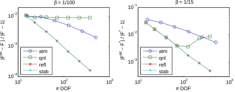
101 102 103 10−4
10−3 10−2
# DOF
|F
ac − F * | / |F * − 1|
β = 1/100
atm qnl
101 102 103
10−3 10−2 10−1
# DOF
|F
ac − F * | / |F * − 1|
β = 1/15
[image:7.595.104.492.62.215.2]atm qnl
Figure 1. Relative errors of critical strains for QNL and the restricted atomistic simulation. The external forces are parameterised by α = 1.5, β ∈ {0.01,0.066}. See
§ A.2 for details of the model and the computation.
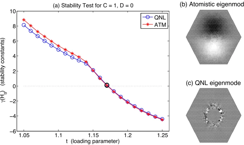
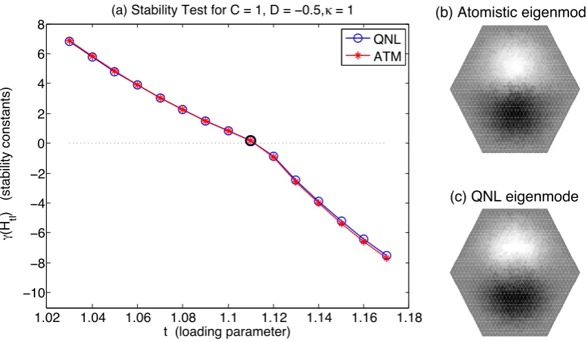
We define the critical strain, Fqnl, to be the smallest strain greater than one, for which the corre-sponding equilibrium yF of the energy is unstable, i.e., γ(δ2Eqnl(yF))≤0.
The exact critical strainF∗, against which the error is measured, is defined to be the critical strain for the unrestricted atomistic model.
In Figure 1 we plot the relative errors in the critical strains, for increasing domain sizes and hence increasing computational cost (measured in terms of the number of degrees of freedom required for the computation) for the QNL method and for the restricted atomistic model. We observe that the critical strains in the restricted atomistic model display clear systematic convergence, whereas the critical strains of the QNL method appear to diverge or converge to a wrong limit.
4. A Universally Stable A/C Coupling in 1D
Motivated by the results of §3 we seek a/c couplings with universally reliable stability properties.
Definition 1. An a/c coupling energy Eac is universally stable if, for all interaction potentials
V ∈C2(RR) and strains F>0,γ(HFac)>0 if and only if γ(HFa)>0.
The analysis in [17] indicates that the behaviour we observed in § 3.3 is not possible if the QNL method were universally stable, and indeed we saw in§3.2 that counterexamples can be constructed. We will now present the construction of a universally stable a/c coupling. For simplicity, we consider again the case where the atomistic region is given by Z− ={0,−1,−2, . . .}. The reflection method, which we formulate in the following paragraphs can be understood as a special case of the QNL and geometric reconstruction ideas [7, 25, 28], but with a particularly simple reconstruction operator.
For any lattice function z : Z → R (both deformations and displacements) we denote its anti-symmetric reflection about the origin by
z∗:=
z(ξ), ξ≤0,
2z(0)−z(−ξ), ξ >0.
With this notation we define, for y=Fx+u, u∈W0,
Erfl(y) :=E∗(y) + Z ∞
0
W(∇y) dx, where
E∗(y) := −1
X
ξ=−∞
V(Dy∗(ξ))−V(FR)+12V(Dy∗(0))−V(FR).
One may readily check that Erfl is of the general form (2.5).
The key property, the reason for the name “reflection method”, and in fact the motivation for the definition ofErfl, is the following.
Proof. By definition, y∗ is anti-symmetric about the origin, and consequently,
Dρy∗(ξ) =y∗(ξ+ρ)−y∗(ξ)
=2y∗(0)−y∗(−ξ−ρ)−
2y∗(0)−y∗(−ξ) =−D−ρy∗(−ξ).
Due to the reflection symmetry (2.1) of V, we obtain V(Dy∗(ξ)) = V(Dy∗(−ξ)), which implies the
stated result.
Theorem 4.2. The a/c couplingErfl is force-consistent,
δErfl(Fx), v= 0, (4.1)
and universally stable,
γ(HFrfl) =γ(HFa). (4.2)
Proof. Proof of (4.1): From Lemma 4.1 we obtain
hδE∗(Fx), vi= 21hδEa(Fx), v∗i,
where we note thatv∗ does not necessarily belong toW0, but∇v∗ has compact support and hence the
right-hand side is well-defined. Lemma 12 in [21] implies that
hδEa(Fx), v∗i=W0(F) Z
R
∇v∗(x) dx. (4.3)
(Note that [21, Lemma 12] is in fact a 2D result, however, the 1D variant is proven verbatim using the 1D bond density formula [26, Proposition 3.3]. Alternatively, (4.3) can be proven directly from [26, Proposition 3.1].)
Since ∇v∗ is symmetric about the origin, (4.3) implies that
hδE∗(F), vi= 12W0(F) Z
R
∇v∗(x) dx=W0(F) Z 0
−∞
∇v(x) dx=W0(F)v(0).
Inserting this into the definition ofδErfl, we obtain
hδErfl(F), vi=W0(F)v(0) + Z ∞
0
W0(F)∇v(x) dx= 0.
Proof of (4.2): Applying again Lemma 4.1, as well as the symmetry of ∇v∗, we obtain
hHFrflv, vi=hδ2E∗(F)v, vi+W00(F) Z ∞
0
|∇v|2dx
= 12hδ2Ea(Fx)v∗, v∗i+W00(F)k∇vk2L2(0,∞) ≥ 12γ(HFa)k∇v∗k2L2(
R)+γ(H
c
F)k∇vkL2(0,∞)
=γ(HFa)k∇vk2L2(−∞,0)+γ(HFc)k∇vk2L2(0,∞)≥γ(HFa)k∇vk2L2( R);
that is,γ(HFrfl)≥γ(HFa). Proposition 2.1 shows that this inequality is in fact an equality.
5. Stabilising the 1D QNL Method
5.1. The general strain gradient representation. A key component in previous sharp stability analyses of a/c methods was a decomposition of a/c hessians into the Cauchy–Born hessian and a strain gradient correction [5, 20, 14]. Here, we generalise these representations to general many-body finite range interactions.
Lemma 5.1. Forξ ∈Z, ρ∈ R, define the sets
A(ξ, ρ) :=
{ξ, . . . , ξ+ρ−1}, ρ >0, {ξ+ρ, . . . , ξ−1}, ρ <0.
Then, for ξ∈Z, ρ, ς∈ R,
Dρu(ξ)Dςu(ξ) =
ρς
2|ρ||ς| X
η∈A(ξ,ρ)
X
η0∈A(ξ,ς)
Proof. It is clear from the definitions that
Dρu(ξ) =
ρ |ρ|
X
η∈A(ξ,ρ)
D1u(η),
and therefore,
Dρu(ξ)Dςu(ξ) =
ρς |ρ||ς|
X
η∈A(ξ,ρ)
X
η0∈A(ξ,ς)
D1u(η)D1u(η0).
Applying the identity
D1u(η)D1u(η0) = 12|D1u(η)|2+12|D1u(η0)|2−12|D1u(η)−D1u(η0)|2,
yields the stated result.
Lemma 5.2. Let HFac be of the general form (2.9), then
hHFacu, ui=hHFcu, ui+h∆acF u, ui, (5.1)
where
h∆acFu, ui=
2rcut−1 X
j=1 0
X
ξ=−∞
cj(ξ)|D1u(ξ)−D1u(ξ−j)|2 with (5.2)
cj(ξ) =
X
ρ,ς∈R ρς
2|ρ||ς|
X
η∈Z−
ξ∈A(η,ρ),ξ−j∈A(η,ς)
˜
Vη,ρς(FR).
Proof. Applying Lemma 5.1 to the representation (2.9) of the QNL hessian, we immediately obtain that
hHFacu, ui=X ξ∈Z
c0(ξ)|D1u(ξ)|2+h∆acFu, ui, (5.3)
where ∆acF is of the form (5.2), and c0(ξ) ∈R are some coefficients that still need to be determined. The stated identity for cj(ξ), j ≥1 in the definition of the strain gradient operator ∆acF , follows from a straightforward exchange of summation.
To determinec0(ξ), we first note that (2.6) implies c0(ξ) =W00(F) for ξ ≥1.
To determine the remaining coefficients we apply the force-consistency condition (2.8). We know from (2.8) that
hδEac((F+tG)x), vi= 0 ∀v∈W0,
for all F > 0, G ∈ R and t sufficiently small. Taking the derivative with respect to t, evaluated at
t= 0, yields
hδ2Eac(Fx)Gx, vi= 0 ∀v∈W0,
or, written in terms of the representation (5.3),
X
ξ∈Z
c0(ξ)(G·a1)D1v(ξ) +h∆acFGx, vi= 0,
where we extended the definition of c0(ξ) by c0(ξ) =W00(F) for ξ >0.
Since Gxis an affine function, h∆acF Gx, vi= 0, and hence we obtain that
X
ξ∈Z
c0(ξ)D1v(ξ) = 0 ∀v∈W0.
5.2. The stabilised QNL method. We observed in Lemma 5.2 that the QNL hessian can be written as the Cauchy–Born hessian with a strain gradient correction in the atomistic and interface region. Moreover, due to the “bounded interface condition” (2.7), we know that the strain gradient correction is the same for the QNL and for the reflection hessians, except in a bounded neighbourhood of the interface. More precisely, we can write
hHFqnlu, ui=hHFrflu, ui+
(∆qnlF −∆rflF )u, ui, (5.4) where
(∆qnlF −∆rflF)u, ui=
2rcut−1 X
j=1
−1
X
ξ=ξ1
c0j(ξ)|D1u(ξ)−D1u(ξ−j)|2,
for someξ1 ≤0 that depends onξ0 and on rcut, and for coefficientsc0j(ξ) :=cj(ξ)−crflj (ξ). Ifc
0
j(ξ)≥0 for allξ, then we would obtain that hHFqnlu, ui ≥ hHrfl
F u, ui and hence the QNL method is universally stable.
Ifc0j(ξ)<0 for some j, ξ, then we can redefine astabilised QNL energy
Estab(y) :=Eqnl(y) +κhSu, ui, fory=Fx+u, u∈W0,
whereκ >0 is a stabilisation constant andS is the stabilisation operator defined through
hSu, ui:=
−1
X
ξ=ξ1−2rcut+2
|D−1D1u(ξ)|2. (5.5)
Because the stabilisation involves only second derivatives, this modification does not affect the first-order consistency of the QNL method; see Remark 5.4.
Theorem 5.3. Fix a bounded set F ⊂R (a range of macroscopic strains F of interest). Then there exists a constant κ0 ≥0 such that, for all κ≥κ0 and for all F∈ F, δ2Estab(Fx) is stable if and only
if HFa is stable.
An upper bound onκ0 is given by
κ0 ≤sup
F∈F
X
ρ,ς∈R
(|ρ|+|ς|)2|ρ||ς|sup ξ∈Z−
Vξ,ρς(FR)−Vξ,ρςrfl (F) ,
where Vξrfl is the effective site potential of the reflection scheme.
Proof. We know from Proposition 2.1 that, ifHFa is unstable, then HFstab is unstable, so we only need to prove the converse statement.
Since the reflection method is universally stable, it follows from (5.4) that it is sufficient to prove that
(∆qnlF −∆rflF)u, ui+κhSu, ui ≥0,
forκ sufficiently large. To prove that this is indeed the case, we simply compute an upper bound on
|
(∆qnlF −∆rflF )u, ui|:
h(∆qnlF −∆rflF )u, ui ≤
2rcut−1 X
j=1
−1
X
ξ=ξ1
|c0j(ξ)||D1u(ξ)−D1u(ξ−j)|2
≤
2rcut−1 X
j=1
−1
X
ξ=ξ1
|c0j(ξ)|j
ξ
X
η=ξ−j+1
D−1D1u(η)
2
,
where we used the Cauchy–Schwarz (or, Jensen’s) inequality. Upon reordering the summation, we obtain
h(∆
qnl
F −∆
rfl
F)u, ui ≤
−1
X
η=ξ1−2rcut+2
D−1D1u(η)
2
( 2rcut−1 X
j=max(1,ξ1−η+1)
min(η+j−1,−1)
X
ξ=max(η,ξ1)
|c0j(ξ)|j )
=:
−1
X
η=ξ1−2rcut+2
D−1D1u(η)
2
d0(F, η).
To get an upper bound on this quantity, we next estimate|c0j(ξ)|. Let
m0(ρ, ς) := sup ξ∈Z−
sup
F∈F
|Vξ,ρς−Vξ,ρςrfl |,
then
|c0j(ξ)| ≤ 1
2 X
ρ,ς∈R
X
η∈Z−
ξ∈A(η,ρ),ξ−j∈A(η,ς)
m0(ρ, ς),
and noting that the sum over η is taken over at most min(|ρ|,|ς|) sites and moreover that only the sum over ρ, ς satisfying |ρ|+|ς| ≥j needs to be taken into account, we obtain
|c0j(ξ)| ≤ 1
2 X
ρ,ς∈R |ρ|+|ς|≥j
min(|ρ|,|ς|)m0(ρ, ς).
Inserting this estimate into the definition ofd0(F, η) gives
d0(F, η)≤
2rcut−1 X
j=max(1,ξ1−η+1)
min(η+j−1,−1)
X
ξ=max(η,ξ1) X
ρ,ς∈R |ρ|+|ς|≥j
1
2min(|ρ|,|ς|)(|ρ|+|ς|)m
0(ρ, ς),
where we estimated j ≤ (|ρ|+|ς|). Next, using 12min(|ρ|,|ς|)(|ρ|+|ς|) ≤ |ρ||ς|, and noting that the sum over ξ ranges over at mostj values, we further estimate
d0(F, η)≤
2rcut−1 X
j=max(1,ξ1−η+1)
j X |ρ|+|ς|≥j
|ρ||ς|m0(ρ, ς)
≤ X
ρ,ς∈R
|ρ||ς|m0(ρ, ς)
min(2rcut−1,|ρ|+|ς|) X
j=1
j≤ X
ρ,ς∈R
|ρ||ς|(|ρ|+|ς|)2m0(ρ, ς).
This establishes the estimate forκ0.
Remark 5.4 (Consistency of the stabilised QNL method). If the cost of stabilising the QNL method is a loss in consistency, then little can be gained by the procedure proposed in the foregoing section. However, (ignoring finite element coarsening of the continuum region) it is easy to show that
kδEstab(u)−δEa(u)k
W∗ ≤ kδEqnl(u)−δEa(u)kW∗+ 2κ0kD−1D1uk`2(I),
where I := {ξ1 −2rcut+ 1, . . . ,−1}. That is, the additional consistency error committed by the
stabilisation is of first-order, which is the same as the consistency error of the QNL method [20, 21, 25, 2].
Moreover, the prefactorκ0 is bounded in terms of the partial derivativesVξ,ρς. Having some uniform bound on these partial derivates Vξ,ρς is a prerequisite to obtain a first-order error estimate [21, 25]. For example, for geometric reconstruction type method [28, 7, 25] one can show that these are bounded in terms of a norm on the reconstruction coefficients.
In summary, we can conclude that the stabilisation (5.4) will normally not affect the consistency of
the QNL method.
5.3. Numerical example. We may now revisit the numerical example from § 3.3, and add the universally stable reflection method and the stabilised QNL method to the graph. We choose the QNL stabilisation parameter κ = 0.1 by trial and error. The extension of the two methods to the finite domain used in this experiment is straightforward.
101 102 103 10−4
10−3 10−2
# DOF
|F
ac − F * | / |F * − 1|
β = 1/100
101 102 103
10−3 10−2 10−1
# DOF
|F
ac − F * | / |F * − 1|
β = 1/15
atm qnl refl stab
[image:12.595.104.493.62.215.2]atm qnl refl stab
Figure 2. Relative errors of critical strains for the QNL, REFL and stabilized QNL methods, and external forces parameterised byα= 1.5, β∈ {0.01,0.066}. The stabili-sation parameter for the stabilised QNL method isκ= 0.1.
6. QNL Formulation of a 2D Nearest-Neighbour Scalar Model
In the remainder of the paper we explore possible generalisations of our foregoing results to higher dimensions. We are unable, at present, to provide results of the same generality as in 1D, and we therefore restrict our presentation to the setting of nearest-neighbour many body interactions for scalar displacement fields (e.g., anti-plane displacements) in two dimensions, with a “flat” a/c interface. Already in this simple setting, we will encounter several difficult new issues that must be overcome before focusing on the even more challenging vectorial case, and general interface geometries. (Admitting a wider interaction range does not seem to cause major additional difficulties.)
6.1. Notation for the 2D triangular lattice. Our 2D analysis is most convenient to perform in the setting of the 2D triangular lattice, which we denote by
Λ :=AZ2, where A=
1 cos(π/3) 0 sin(π/3)
.
For future reference, we define the six nearest-neighbour lattice directions by a1 := (1,0), andaj := Qj6−1a1,j∈Z, where Q6 denotes the rotation through angle 2π/6 and we note that aj+3 =−aj.
For a lattice functionw: Λ→R, we define the nearest-neighbour differences
Djw(ξ) :=w(ξ+aj)−w(ξ).
The interaction range is defined asR={a1, . . . , a6}and the corresponding finite difference stencil by
Dw(ξ) ={Djw(ξ)}6
j=1.LetkDwk`2 := (Pξ∈ΛPj3=1|Djw(ξ)|2)1/2.
Let T denote the canonical triangulation of R2 with nodes Λ, using closed triangles, then each lattice function v is identified with its continuous piecewise affine interpolant with respect to T. In particular, we define ∇vT to be the gradient of v in T ∈ T and we note that ∇vT ·aj = Djv(ξ) if
ξ, ξ+aj ∈T.
The space of admissible test functions is again the space of compactly supported lattice functions, defined by
W0:=
u: Λ→R
supp(u) is bounded .
For an operatorH :W0→W0∗ we define againγ(H) := infu∈W0,k∇ukL2=1hHu, ui.
6.2. 2D many-body nearest neighbour interactions. We fix a nearest-neighbour many-body (i.e., 7-body) potential V ∈C2(R6), with partial derivatives
Vi(g) =
∂V(g)
∂gi
and Vij(g) =
∂2V(g)
∂gi∂gj
forg= (gi)6i=1∈R6.
For a deformed configuration y = F·x+u (where x(ξ) = ξ and F ∈ R2) we define the energy
difference by
Ea(y) =X ξ∈Λ
V(Dy(ξ))−V(FR)
Since the sum is effectively finiteEa is well-defined and admits two variations in the sense of Gateaux
derivatives, with the second variation given by
hδ2Ea(y)v, vi=X
ξ∈Λ 6
X
i,j=1
Vij(Dy(ξ))·Div(ξ)Djv(ξ).
We are again particularly interested in homogeneous states y(x) =Fxand define
hHFau, ui=X ξ∈Λ
6
X
i,j=1
Vij ·Diu(ξ)Dju(ξ), (6.2)
where, here and throughout we omit the argument FR inVij when it is clear from the context that we mean Vij(FR).
6.2.1. Symmetries. Inversion symmetry about each lattice point leads us to assume thatV((gi)6i=1) =
V((−gi0)6
i=1), wherei0 ∈ {1, . . . ,6}such thatai0 =−ai. This yields the point symmetry for the second
derivatives Vi,j(FR) = Vi0,j0(FR) fori, j ∈ {1, . . . ,6}; see, e.g., [24]. Since the reference lattice Λ has
full hexagonal symmetry, it is reasonable to make the stronger assumption thatV has full hexagonal symmetry as well, i.e.,
V(g) =V(g6, g1, . . . , g5). (6.3)
In this case, but only for the deformationF=0, one can readily deduce the identities
V1,1 =· · ·=V6,6=:α0,
V1,2 =· · ·=V5,6 =V6,1=:α1,
V1,3=· · ·=V4,6 =V5,1 =V6,2=:α2, and
V1,4 =V2,5 =V3,6=:α3,
(6.4)
whereVi,j =Vi,j(0) and αi ∈R.
Both symmetries can be derived, e.g., by reducing a 3D model to a scalar 2D anti-plane model.
6.3. QNL-type methods. We define the Cauchy–Born approximation in a discrete sense,
Ec(y) := 1
2 X
T∈T
W(∇yT)−W(F) ,
whereW(F) :=V(FR). Unusually, we have not normalisedW with respect to volume, which somewhat simplifies notation. (Since each site has associated volume 1, each element has associated volume 3/6 = 1/2.)
We define the atomistic and continuum lattice sites
Λa :={ξ∈Λ|ξ2 <0}, Λc:={ξ∈Λ|ξ2 >0},
and in addition the kth “row” of atoms Λ(k) :=
ξ ∈Λξ2 =k √
3/2 ,
so that Λ(0) is the set of interface lattice sites.
QNL methods are a/c coupling schemes with energy functional of the form
Eqnl(y) := X ξ∈Λa
V(Dy(ξ))−V(FR)
+ X
ξ∈Λ(0) ˜
V(Dy(ξ))−V(FR)
+ X
ξ∈Λc
1 3
X
T∈T
ξ∈T
W(∇yT)−W(F)
,
(6.5)
where ˜V is a modified interaction potential that is chosen to transition between the atomistic and Cauchy–Born description. For more detail we refer to [28, 7, 21] and in particular [25] which is closest in terms of analytical setting and notation to our present work.
We assume throughout that ˜V ∈C2(R6), then the QNL energy is well-defined fory=F·x+u, u∈
W0, and has two variations in the sense of Gateaux derivatives.
We assume thatEqnl does not exhibit ghost forces,
and isenergy-consistent,
˜
V(FR) =V(FR) ∀F∈R2. (6.7)
Sometimes, to achieve a more compact notation, we write
Eqnl(y) = X ξ∈Λa∪Λ(0)
˜
Vξ(Dy(ξ))−V(FR)
+ X
T∈T wT
W(∇yT)−W(F)
,
where ˜Vξ = ˜V forξ∈Λ(0), ˜Vξ=V forξ ∈Λa, andwT = #(Λc∩T)/6. The second variation (hessian) aty=Fx,HFac=δ2Eqnl(Fx), is then given by
hHFacu, ui= X ξ∈Λa∪Λ(0)
6
X
i,j=1
˜
Vξ,ij·Diu(ξ)Dju(ξ) +
X
T∈T
wT(∇uT)>W00(F)∇uT, (6.8)
whereW00(F)∈R2×2 is the hessian of W.
As in the foregoing 1D results we shall focus exclusively on stability at homogeneous states. We show in [22, Appendix A.6] how one may extend such results to stability of non-homogeneous states including defects.
We remark that the 2D variant of Lemma 2.3,γ(HFa)≤γ(HFc), remains true [10].
To illustrate that we are not talking about abstract methods, but concrete practical formulations we now introduce three specific variants.
6.3.1. The QCE method. The simplest QNL variant is the QCE method [19, 3], which is defined by simply taking ˜V =V. It is shown in [25] that in our present setting (nearest neighbour interaction, flat interface) it satisfies the force-consistency condition (6.6).
We denote the resulting energy functional byEqce.
6.3.2. The GRAC-2/3 method. The QCE method doesnotsatisfy the force consistency condition (6.6) in domains with corners, nor for second neighbour interactions [27, 28, 7, 3, 25] and it is still an open problem to formulate a general scheme that does. A class of methods has been introduced in [25], extending ideas in [28, 7], which in our context can be defined through
˜
V(Dy) :=V( ˜Dy), where D˜iy:=λiDi−1y+ (1−λi)Diy+λiDi+1y,
for λi ∈R. It is shown in [25] that, for flat interfaces, all of these schemes satisfy (6.6), and for the choice
λi=
1/3, i= 2,3 0, i= 1,4,5,6 ,
(and only for this choice) the resulting method (GRAC-2/3) can be extended to domains with corners while still satisfying (6.6). We denote the resulting energy functional by Eg23.
6.3.3. The local reflection method. Finally, we introduce a new a/c coupling scheme, inspired by our 1D reflection method.
The idea is to apply the reflection method on each site ξ∈Λ(0), which amounts to defining
˜
Di :=
Di, i= 1,4,5,6
−Di+3, i= 2,3, and
˜
V(Dy) := 1
2V( ˜Dy) + 1 6
X
T∈Tc
ξ∈T
W(∇yT),
whereTc:={T ∈ T |x
2≥0 for allx∈T}.
The idea can be seen more clearly, if we write the resulting energy functional in the form
Elrf(y) := X ξ∈Λa
V(Dy(ξ))−V(FR)+1 2
X
ξ∈Λ(0)
V( ˜Dy(ξ))−V(FR)+ 1 2
X
T∈Tc
W(∇yT)−W(F)
.
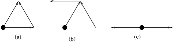
(a) (b) (c)
Figure 3. Visualisation of the identities (6.9)–(6.11). The bullets denote the sites ξ, while the arrows denote the terms|Dju(η)|2 occuring in these identities. (a) visualises
(6.9); (b) visualises (6.10); (c) visualises (6.11).
6.4. Atomistic and Cauchy–Born hessian representations. Our aim is to develop a generalisa-tion of our 1D hessian representageneralisa-tion, Lemma 5.2. Towards this end, we first establish representageneralisa-tions for the atomistic and Cauchy–Born hessians. The result for the QNL hessian will be presented in§7. We first state two auxiliary lemmas. The first provides a mechanism for establishing whether two symmetric bilinear forms are equal.
Lemma 6.1. Let H1, H2 be self-adjoint operators defined through
hHiu, ui=
X
ξ∈Λ 3
X
j=1
hi,j(ξ)|Dju(ξ)|2,
thenH1 =H2 if and only if h1,j(ξ) =h2,j(ξ) for all ξ∈Λ, j= 1, . . . ,3.
Proof. For some η ∈ Λ and j ∈ {1,2,3}, we define u(ξ) = δξ,η and v(ξ) = δξ,η+aj, where δ is the Kronecker delta. Then the productDku(ξ)Dkv(ξ) is non-zero if and only ifξ =η and k=j. Hence,
0 =h(H1−H2)u, vi=−(h1,j(η)−h2,j(η)).
Hence we conclude that h1,j(η) = h2,j(η) for all η ∈ Λ and j = 1,2,3. The converse implication is
trivial.
In the “canonical” hessian representations ofEa,Ec,Eqnlproducts of finite differencesD
iu(ξ)Dju(ξ) occur; see (6.2) and (6.8). In 1D, we converted these products into squares of strains and strain gradients. The next lemma provides an analogous representation for general mixed differences. In [22, Appendix A.4] we provide the generalisation for general finite range interaction.
Lemma 6.2. Let u∈W0,ξ ∈Λ andi∈ {1, . . . ,6}, then
Diu(ξ)Di+1u(ξ) = 12|Diu(ξ)|2+12|Di+1u(ξ)|2−12|Di+2u(ξ+ai)|2, (6.9)
Diu(ξ)Di+2u(ξ) = 12|Di+1u(ξ)|2−12|Di+2u(ξ+ai)|2 (6.10)
−1
2|Di+3u(ξ+ai+1)| 2+1
2|DiDi+2u(ξ)| 2,
Diu(ξ)Di+3u(ξ) =−12|Diu(ξ)|2−21|Di+3u(ξ)|2+12|Di+3Diu(ξ)|2. (6.11)
Proof. All three identities are straightforward to verify by direct calculations.
Proposition 6.3 (Cauchy–Born Hessian). There exist cj =cj(F), j= 1,2,3, such that
hHFcu, ui=
3
X
j=1
cj
X
ξ∈Λ
|Dju(ξ)|2,
where W00(F) = 12P3
j=1cjaj⊗aj.
In the hexagonally symmetric case (6.4), we have c1 =c2 =c3 =:c.
Proof. The result can be checked by a straightforward calculation. The complete proof is given in [22,
Next, we establish the “strain-gradient” representation of the atomistic hessian. We define a sum of squares p :RK → R to be a diagonal homogeneous quadratic, i.e., a function of the form p(z) = PK
k=1ckzk2.
Proposition 6.4. There exists a sum of squaresX =XF :R36→R, such that
hHFau, ui=hHFcu, ui+X ξ∈Λ
X(D2u),
where D2u(ξ) = (DiDju(ξ))6i,j=1.
Proof. Applying the identities (6.9)–(6.11) to the original form (6.2) ofHFa, and noting the translation invariance of these operations, we obtain
hHFau, ui=
3
X
j=1
cajX
ξ∈Λ
|Dju(ξ)|2+X ξ∈Λ
X(D2u(ξ)),
whereX(D2u) =P
i,jbij|DiDju|2 for some coefficients bi,j ∈R. It only remains to show thatcaj =cj forj= 1,2,3.
To prove this, we use a scaling argument. Let u ∈ C0∞(R2), and let u(ε)(ξ) := εu(εξ), then it is elementary to show that
2
√
3
HFcu(ε), u(ε)→ Z
R2
3
X
j=1
cj|∇u·aj|2dx=
Z
R2
∇uTC∇udx, and
2
√
3
HFau(ε), u(ε) →
Z
R2
3
X
j=1
caj|∇u·aj|2dx=
Z
R2
∇uTCa∇udx,
whereC=P3
j=1cjaj⊗aj andCa =
P3
j=1cajaj⊗aj. (The factor 2/
√
3 accounts for the density of lattice sites.) Moreover, since HFc is the hessian of the Cauchy–Born continuum model, restricted to a P1 finite element space, we know that the two limits must be identical,R
∇uTC∇udx=R
∇uTCa∇udx,
which is only possible if C = Ca. Since the three rank-1 matrices aj ⊗aj, j = 1,2,3, are linearly
independent, we can conclude thatcj =caj forj = 1,2,3.
6.5. Simple cases. 1. Suppose that the potentialV is such thatVi,i+2=Vi,i+3 ≡0 for alli= 1, . . . ,6;
that is, only the “neighbouring bonds” interact. (In the hexagonally symmetry case, this amounts to assuming that α2 =α3 = 0.) This could, for example, be understood as a simple case of bond-angle
interaction. Then, in the proof of Proposition 6.4, only the identity (6.9) is employed but neither (6.10) nor (6.11). Therefore, X≡0, and we obtain that Ha
F =HFc.
2. In the hexagonally symmetric case (6.4), without assuming α2 = α3 = 0, a straightforward
explicit computation yields
c= 2(α0+α1−α2−α3), and (6.12)
X(D2u) =
6
X
i=1
α2|Di+2Diu|2+α3|Di+3Diu|2
.
7. Instability and Stabilization in 2D
In this section we will derive the “strain gradient” representation of the QNL hessian. We shall find that, in contrast to our one-dimensional result (Lemma 5.2), in 2D there is a source of instability that is different from an error in the strain gradient coefficients, and therefore more severe.
7.1. QNL hessian representation. Applying the rules (6.9)–(6.11) to the “canonical” QNL hessian representation (6.8) we obtain the following result.
Proposition 7.1. There exist coefficients ˜cj(ξ) = ˜cj(F, ξ), and sums of squares X˜ξ :R36→ R such that
hHFacu, ui=
3
X
j=1
X
ξ∈Λ
˜
cj(ξ)|Dju(ξ)|2+
X
ξ∈Λ
˜
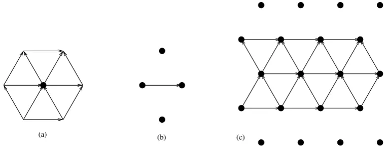
(c)
[image:17.595.107.490.57.204.2](a) (b)
Figure 4. (a) Bonds (arrows) that are affected by the operations (6.9)–(6.11), from a single size ξ (black disk); (b) Sites (black disks) that affect a given bond (arrow) through the operations (6.9)–(6.11). (c) Bonds for which the coefficients ˜cj(ξ) of the a/c hessian differ from the coefficientscj of the Cauchy–Born hessian; cf. Proposition 7.1.
Moreover, the following identities hold:
˜
cj(ξ) =cj except if bothξ, ξ+aj ∈Λ(−1)∪Λ(0)∪Λ(1), (7.2) ˜
Xξ = 0 for ξ2 >0, and (7.3)
˜
Xξ=X for ξ2 <0. (7.4)
Proof. Applying the identities (6.9)–(6.11) to the hessian representation (6.8) we obtain (7.1), and it only remains to prove (7.2)–(7.4).
The identities (7.3) and (7.4) simply follow from the fact that the operations (6.9)–(6.11) only create strain gradient terms associated with the centre atomξ.
The remaining property (7.2) can be obtained by understanding which bond coefficients ci(η) are “influenced” by the operations (6.9)–(6.11) applied with a given centre atomξ. These are depicted in Figure 3 and after combining the graphs for the three identities and rotating them, we see that a lattice siteξ only influences the coefficientsci(η) corresponding to the twelve bondsDju(ξ), j= 1, . . . ,6 and
Dj+2u(ξ +aj), j = 1, . . . ,6; cf. Figure 4 (a). From this, it follows that a given coefficient ci(η) is influenced only by the four nodes of the two neighbouring triangles; cf. Figure 4 (b). Thus, only the bonds depicted in Figure 4 (c) are affected by the modified site potentials, which are precisely those bonds contained in the strip {x∈R2| −
√
3/2≤x2 ≤
√
3/2}.
Although we have always restricted our presentation to the flat interface situation, all results up to this point are generic. That is, they can be generalised to interfaces with corners and even to long range interactions.
In the next result, where we provide some characterisation of the coefficients ˜cj(ξ) in the interface region, we exploit tangential translation invariance.
Lemma 7.2. Suppose that the modified site-energies are tangentially translation invariant, i.e., ˜
Vξ= ˜Vξ+a1 for all ξ∈Λ
(0). Then the coefficients in the strain gradient representation (7.1)satisfy
˜
cj(ξ) =cj for allξ ∈Λ, j= 2,3. (7.5)
Moreover, for j = 1 and ξ ∈ Λ(m), m = −1,0,1, we have ˜c1(ξ) = ˜c(1m) (tangential translation
invariance) and
1
X
m=−1
˜
c(1m) = 3c1. (7.6)
Proof. 1. Properties ofc˜2,˜c3: By the same argument as in the 1D case (cf. Lemma 5.2) we can prove
that
We fixξ ∈Λ and test (7.7) with u(η) :=δξ,η (i.e., a “hat-function”) to obtain
3
X
j=1
˜
cj(ξ)(−G·aj) +
3
X
j=1
˜
cj(ξ−aj)(G·aj) = 0.
If we define cj+3(ξ) :=cj(ξ−aj) for j= 1,2,3, then this can equivalently be stated as
−G·
6
X
j=1
˜
cj(ξ)aj = 0.
Since this must hold for allG∈R2, we deduce that 6
X
j=1
˜
cj(ξ)aj = 0 ∀ξ∈Λ. (7.8)
Using that fact thataj+3=−aj and a1+a3+a5 = 0, we deduce that (7.8) is equivalent to
˜
c1(ξ)−c˜4(ξ) = ˜c3(ξ)−˜c6(ξ) = ˜c5(ξ)−c˜2(ξ) ∀ξ∈Λ. (7.9)
We now test (7.9) with ξ ∈Λ(1). Due to the translation invariance of the modified site-energies it follows that ˜c1(ξ) = ˜c4(ξ). Moreover, ˜c3(ξ) =c3 and ˜c2(ξ) =c2, which implies that
0 =c3−c˜6(ξ) = ˜c5(ξ)−c2.
This implies (7.5) forξ ∈Λ(0). Analogously, testing (7.9) withξ ∈Λ(−1) gives (7.5) forξ ∈Λ(−1). Properties of c˜1: We are left to establish the statements concerning the coefficients ˜c1. Due to
translation invariance of the site potential it immediately follows that ˜cj(ξ) = ˜cj(ξ+a1), hence we can
write ˜cj(ξ) = ˜c(jm) forξ ∈Λ(m),m=−1,0,1.
Finally, (7.6) is a consequence of the energy consistency (6.7). If we allowed noncompact test functions (as, e.g., in a periodic setting), then we could take the second variation ofEa(Fx) =Eqnl(Fx)
along the displacement u = Gx and obtain hHa
FGx,Gxi = hH
qnl
F Gx,Gxi which would imply (7.6). However, in our caseGx /∈W0, which makes the proof of (7.6) more involved.
We start with noticing that the energy consistency implies
6
X
i,j=1
( ˜Vi,j−Vi,j)Diu(ξ)Dju(ξ) = 0
foru=Gx and some ξ∈Λ(0). We then rewrite this using the rules (6.9)–(6.11) as
3
X
i=1
X
ρ∈Λ
ρ,ρ+ai∈R∪{0}
(˜ci,ρ−ci,ρ)|Diu(ξ+ρ)|2+ ˜X(D2u(ξ))−X(D2u(ξ)) = 0
with some ˜ci,ρ and ci,ρ. Next, we substituteu=Gx and useD2(Gx) = 0:
3
X
i=1
X
ρ∈Λ
ρ,ρ+ai∈R∪{0}
(˜ci,ρ−ci,ρ)|Gai|2 = 0. (7.10)
It remains to notice that, since ˜c(im) and ci were constructed using the same rules as ˜ci,ρ and ci,ρ, we have
X
ρ∈Λ
ρ,ρ+ai∈R∪{0}
(˜ci,ρ−ci,ρ) =
1
X
m=−1
(˜c(im)−ci) (i= 1,2,3).
Substituting this into (7.10) and using that ˜c(im) =ci(m) fori= 2,3, we get
1
X
m=−1
(˜c(1m)−c1)|Ga1|2 = 0
We see that the key difference, between 1D and 2D, for the stability of homogeneous deformations is that the |Dju|2 coefficients in the 1D case are identical to those in the Cauchy–Born model for
force-consistent a/c couplings, while this need not be the case in 2D. As a first step to showing that this can lead to an instability in 2D, we establish another representation of HFqnl.
Lemma 7.3. Under the conditions of Lemma 7.2, we have
hHFqnlu, ui=hHFcu, ui+ 2 ˜c(1)1 −˜c(1−1)hK0u, ui+X ξ∈Λ
ˆ
Xξ(D2u(ξ)), (7.11)
where Xˆξ are quadratic forms of D2u (not necessarily sums of squares), with Xˆξ= 0 for ξ ∈Λc, and
hK0u, ui:= X ξ∈Λ(0)
D2D1u(ξ)D1u(ξ).
Proof. From Lemma 7.2 we have
hHFqnlu, ui − hHFcu, ui −X
ξ∈Λ
˜
Xξ(D2u(ξ))
= ˜c(1)1 −c1
X
ξ∈Λ(0)
|D1u(ξ+a2)|2− |D1u(ξ)|2
+ ˜c(1−1)−c1
X
ξ∈Λ(0)
|D1u(ξ+a5)|2− |D1u(ξ)|2
= ˜c(1)1 −c1
X
ξ∈Λ(0)
D1u(ξ+a2)−D1u(ξ)
D1u(ξ+a2) +D1u(ξ)
+ ˜c(1−1)−c1
X
ξ∈Λ(0)
D1u(ξ+a5)−D1u(ξ)
D1u(ξ+a5) +D1u(ξ)
= ˜c(1)1 −c1
X
ξ∈Λ(0)
D2D1u(ξ) (2D1u(ξ) +D2D1u(ξ))
+ ˜c(1−1)−c1
X
ξ∈Λ(0)
D5D1u(ξ) (2D1u(ξ) +D5D1u(ξ))
= (˜c(1)1 −˜c(1−1)) X ξ∈Λ(0)
D2D1u(ξ)D1u(ξ)
−(˜c(1−1)−c1)
X
ξ∈Λ(0)
D5D2D1u(ξ)D1u(ξ) +. . . ,
where “. . .” stands for some sum of squares of D2u(ξ). Summation by parts,
X
ξ∈Λ(0)
D5D2D1u(ξ)D1u(ξ) =−
X
ξ∈Λ(0)
D5D2u(ξ)D4D1u(ξ)
completes the proof.
7.2. Non-existence of a universally stable method in 2D. Lemma 7.3 suggests that, unless ˜
c(1)1 −c˜(1−1) = 0, there is a discrepancy between HFqnl and HFc that is not a quadratic in D2u (and, as will be shown in§7.3, unavoidably leads to an instability). We next establish that in fact ˜c(1)1 −˜c(1−1)6≡0 for a large family of a/c schemes, which not only includes examples from §6.3 but also all geometric reconstruction type variants [7, 25]. Below, we also present in explicit calculations for the three methods from §6.3.
Proposition 7.4. Consider the following generalization of the geometric reconstruction a/c (GRAC) method[25]:
˜
V(g) = L
X
`=1
where w` ∈ R, w` 6= 0, and C` ∈R6×6 (` = 1, . . . , L). Assume that it satisfies the force and energy consistency conditions (6.6),(6.7). Further, assume hexagonal symmetry (6.4)ofV, withα2 =α3= 0.
Then, there exist p0, p1 ∈R (depending on w`,C`) such that p0−p1 = 1 and
˜
c(1)1 −c˜(1−1) =p0α0+p1α1.
In particular, there exists no choice of method parameters w`,C`, such that c˜
(1) 1 −˜c
(−1)
1 = 0 for all
parameters (α0, α1).
Proof. Step 1 (reduction to a GRAC).Consider a method with interface site potential
˜ ˜
V(g) :=V(Bg), (7.13)
whereB:=PL
`=1w`C`. We show that it is energy and force consistent and moreoverhδ2V˜(FR)u, ui −
hδ2V˜˜(FR)u, ui is a sum of squares ofD2u (and hence ˜c(1) 1 −˜c
(−1)
1 is the same for both methods).
Indeed, substituting V(g) =v0+f ·g into the energy consistency condition (6.7) yields
v0
L
X
`=1
w`−1
+f ·(BFR −FR) = 0 ∀v0 ∈R, ∀f ∈R6 ∀F∈R2.
Hence we getPL
`=1w`= 1 andBFR=FRfor allF. These identities make it straightforward to verify the energy and force consistency of (7.13), given the energy and force consistency of (7.12).
Finally, to show that δ2V˜(FR)−δ2V˜˜(FR)u, uis a sum of squares ofD2u, compute
δ2V˜(FR) = L
X
`=1
w`C>`HC`, (7.14)
whereH:=δ2V(FR)∈R6×6 is the hessian of V. We apply the identity
w`C>`HC`+wjC>jHCj = (w`+wj) w`wC``++wwjjCj
>
H w`C`+wjCj
w`+wj
+ wjw`
w`+wj(C`−Cj) >H(C
`−Cj)
to (7.14) L−1 times, noticing that the finite difference operator (C` −Cj)Du is zero on all affine functions and hence can be represented as a sum of second differences. As a result, we express
δ2V˜(FR) as δ2V˜˜(FR) plus squares of second differences.
Step 2 (proof for a GRAC). It is now sufficient to establish this proposition for a simpler method (7.13). Using the rules (6.9)–(6.11), we can express
˜
c(1)1 −c˜(1−1) =−1
3(α0+ 4α1) + ˜V˜1,3+ ˜V˜2,3+ ˜V˜2,4−
˜ ˜
V4,6−V˜˜5,6−V˜˜5,1,
which implies linearity of ˜c(1)1 −˜c(1−1) with respect toα0 and α1, that is, ˜c(1)1 −c˜ (−1)
1 =p0α0+p1α1.
To see thatp0−p1= 1, choose coefficientsα0 = 1 andα1 =−1, i.e., so thatp0−p1= ˜c(1)1 −˜c (−1)
1 ).
In this case the hessian ofV is given by
H=δ2V(FR) =
−1 1 0 0 0 1
1 −1 1 0 0 0
0 1 −1 1 0 0
0 0 1 −1 1 0
0 0 0 1 −1 1
1 0 0 0 1 −1
(7.15)
and δ2V˜˜ =B>HB. Next, denote the column-vectors of Basbi ∈R6 and hence express
˜
c(1)1 −˜c(1−1)= 1 +b>1Hb3+b>2Hb3+b>2Hb4−b>4Hb6−b>5Hb6−b>5Hb1
(here we used 13(α0+ 4α1) =−1).
Energy consistency (6.7) implies P6
i=1(Fai)bi = (Faj)6j=1 (we refer to [25] for details). Using this
identity with F= 23(a6+a1)> and withF= 23(a2+a3)> allows to express
b1 =b3+b4−b6+ (1,0,−1,−1,0,1)> and b2=b5+b6−b3+ (0,1,1,0,−1,−1)>.
Substituting these expressions into ˜c(1)1 −c˜(1−1) yields, after all cancellations,
˜
c(1)1 −c˜(1−1) = 1 + (1,0,−1,−1,0,1)H(b3−b5) + (0,1,1,0,−1,−1)H(b3+b4),
Remark 7.5. Suppose that (in some practical problem)F=F0 is fixed and given a priori.
1. One can then consider energy consistent methods with ghost-force correction, such as [19] (i.e., methods that satisfy (6.6) only for F =F0). Since we do not use explicitly force consistency (6.6) in
the proof, Proposition 7.4 would also be valid for such methods.
2. Nevertheless, it is possible to precompute ˜c(1)1 −˜c(1−1) and subtract the term 12(˜c(1)1 −c˜(1−1))((g2−
g3)2−(g5−g6)2) from ˜V(g), thus correcting the error in ˜ci(ξ). We will, however, not pursue in this work the questions of applicability of such correction beyond the nearest-neighbour plane-interface scalar setting.
3. For the three concrete schemes we introduced in § 6.3, in the fully symmetric case with α2 =
α3= 0, we obtain the following formulas (see [22, Appendix A.3] for proofs):
hHqceu, ui=hHau, ui+α0+ 4α1
3
X
ξ∈Λ(0)
|D1u(ξ)|2− |D
1u(ξ+a2)|2
,
hHlrfu, ui=hHau, ui−α1
X
ξ∈Λ(0)
|D1u(ξ)|2− |D1u(ξ+a5)|2
+ X
ξ∈Λ(0)
Xlrf(D2u(ξ)), and
hHg23u, ui=hHau, ui+ (α0+ 2α1)
X
ξ∈Λ(0)
|D1u(ξ)|2− |D1u(ξ+a2)|2
+ X
ξ∈Λ(0)
Xg23(D2u(ξ)).
7.3. Instability. It is fairly staightforward to see that γ(K0) = γ(−K0) < 0 (cf. (7.11)). In this
section we will show that the strain gradient correction (third group) in (7.11)) cannot improve this indefiniteness of K0, which will immediately imply the instability result (Corollary 7.7).
The strain gradient correction is clearly bounded by an operator of the form
hSu, ui:= X
ξ∈Λ(0)
|D2u(ξ)|2, (7.16)
that is,|Xˆξ(D2u)| ≤C|D2u(ξ)|2. We therefore consider generic operators of the form
hKκu, ui:=hK0u, ui+κhSu, ui. (7.17)
We will show thatKκ is indefinite, independent of the choice ofκ, and hence independent of the form the strain gradient correction ˆXξ takes. Note that this result is also a preparation for our analysis of the 2D analogue of the stabilisation (5.2).
Lemma 7.6. There exists a constant c >0 such that
inf u∈W0 kDuk`2=1
hKκu, ui=:λκ ≤ −
c
(κ+ 1)2. (7.18)
Proof. To obtain this bound, we make a separation of variables ansatz,
u(ξ) =u(ma1+na2) =αmβn,
and we defineα0m:=αm+1−αm, α00m:=αm+1−2αm+αm−1, and analogous notation for β.
Next, letA, B∈C∞(R) be compactly supported withB(0) = 1, andB0(0) = 1, B00(0) = 0.
Let N ∈ N and define αm := A(m/N) and βn := B(n/N), then simple scaling arguments show that, forN ≥N0 (sufficiently large),
β00 ≈N−1, |β000|.N−4,
kαk2`2 ≈NkAk2L2, kα0k2`2 ≈N−1kA0k2L2, kα00k2`2 ≈N−3kA00k2L2,
and analogous bounds for β in terms of B. Here and for the remainder of the proof, “≈” indicates upper and lower bounds up to constants that are independent of κ, N.
With these definitions and derived properties we obtain (after some work) that
hK0u, ui=−β00kα
0k2
`2 ≈ −N−2,
hSu, ui ≈ |β0|2kα00k2`2+|β00|2kα0k2`2 ≈N−3, and kDuk2
that is,
λκ ≤
hKκu, ui
kDuk2
`2
≤ −C1N−2+C2κN−3,
whereC1, C2 >0 depend onA, B but are independent of κ and ofN (provided N ≥N0).
Ifκ= 2C1
3C2N0 =:κ0, choosingN =N0, we obtainλ(κ)≤ −
C1
3 N
−2 0 .
Forκ > κ0, letN = 32CC21κ, thenN ≥N0 and this implies thatλκ ≤ −274C13C
−2
2 κ−2. This completes
the proof.
We can deduce the following instability result. Ignoring the (non-trivial) technical conditions, the result can be read as follows: if the error in the coefficients ˜c(1m) does not cancel at a critical strainG (whereHGa becomes unstable) then the QNL method will necessarily predict a reduced critical strain with an O(1) error. That is, the critical deformation G cannot be predicted with arbitrarily high accuracy by the QNL method. See§ 2.3.1 for further discussion of this issue.
Corollary 7.7. Consider the hexagonally symmetric case (6.4) with α2 = α3 = 0. Suppose,
moreover, that
(i) γa(0) = 0, and that (ii) ˜c(1)1 (0)−˜c(1−1)(0)6= 0. Then, γqnl(0)<0.
In particular, γqnl(G)<0 for sufficiently small |G|.
Proof. The symmetry assumptions and (i) imply that H0a =H0c = 0. Therefore, applying (7.11) we obtain that
hH0qnlu, ui ≤2(˜c(1)1 −c˜(1−1))hK0u, ui+κhSu, ui
for someκ >0. Lemma 7.6 implies that γqnl(0)<0.
Remark 7.8. 1. In the above corollary, (i) is an assumptions onV, whereas (ii) is the assumption on an a/c scheme. We showed in §7.4 that (ii) is generically satisfied.
2. Our numerical investigations (§§8.1 and 8.2) indicate that similar results hold for more general
V and G, i.e., not necessarily satisfying G=0and the simplifying conditionα2=α3 = 0. It does not,
however, appear straightforward to extend our analysis.
7.4. Stabilising the 2D QNL Method. To conclude our analysis of the 2D case, we explore the issue of stabilisation. Let S be given by (7.16) then we define the stabilised QNL energy functional
Estab(y) :=Eqnl(u) +κhSu, ui, (7.19) for someκ≥0.
A consequence of Corollary 7.7 is that (under its technical conditions), for any fixedκ, ifγ(Ha
G) = 0 then γ(HGstab) < 0, that is, the critical deformation G can still not predicted with arbitrarily high accuracy. However, there is some hope that the error can be controlled in terms of κ. To that end, we first show that Lemma 7.6 is in fact sharp.
Theorem 7.9. Let Kκ and λκ be defined by (7.17), then there exist constants c1, c2>0 such that
− c1
(κ+ 1)2 ≤λκ≤ −
c2
(κ+ 1)2 ∀κ≥0. (7.20)
Proof. The upper bound has already been established in Lemma 7.6, hence we only have to show that it is sharp. Forκ≤1, the lower bound is obvious, hence we assume thatκ >1.
We first (crudely) estimate
hKκu, ui ≥ X
ξ∈Λ(0)
D2D1u(ξ)D1u(ξ) +κ 6
X
i=1
|DiD1u(ξ)|2
≥ X
ξ∈Λ(0)
−41κ|D1u(ξ)|2+κ|D21u(ξ)|2
If we can prove the trace inequality
kD1uk2`2(Λ(0))≤C1
κ2kDD1uk2`2(Λ(0))+κ
−1kDuk2
`2(Λ)
, (7.21)
for some constantC1, which can equivalently be rewritten as
− 1 4κ
D1u
2
`2(Λ(0))+κ DD1u
2
`2(Λ(0))≥ −
c1
κ2kDuk
2
`2(Λ),
then the stated result follows.
Proof of (7.21): It turns out that (7.21) is a consequence of the embedding ˙H1(
R2)→ H˙1/2(R). To make this precise we resort to Fourier analysis. Let
ˆ
u(k) := X ξ1∈Z
u(ξ1,0)eikξ1,
then ˆu is a periodic smooth function on (−π, π) and the following bounds hold:
kD1uk2`2(Λ(0))≈ Z π
−π
|k|2|u|ˆ2dk,
kD12uk2`2(Λ(0))≈ Z π
−π
|k|4|u|ˆ2dk, and
kDuk2`2(Λ)& Z π
−π
|k||u|ˆ2dk. (7.22)
The first two bounds are completely standard. The bound (7.22) is a discrete variant of a standard trace inequality (see [22] for a proof).
We thus deduce that, to prove (7.21) it is sufficient to show that there exists C10 such that
k2 ≤C10 κ2k4+κ−1|k|
∀k∈[−π, π].
But, in fact, it is easy to see that k2≤max(κ2k4, κ−1|k|), and hence (7.21) follows.
We can now refine the discussion at the beginning of the section to obtain the following result.
Corollary 7.10. Let V have hexagonal symmetry (6.4), Vi,i+2 =Vi,i+3 ≡0, and ˜c(1)1 −˜c (−1)
1 6= 0;
then there exists constants c1, c2 >0 such that
γ(H0a)− c1
κ2 ≤γ(H qnl
0 +κS)≤γ(H
a
0)−
c2
κ2.
Proof. The result is an immediate consequence of Theorem 7.9.
To explain the relevance of Corollary 7.10 consider the setting of § 2.3.1 and suppose, for the sake of argument, that the result holds at the critical strain,
γ(HGa(t∗))− c1
κ2 ≤γ(H qnl
G(t∗)+κS)≤γ(H
a
G(t∗))−
c2
κ2.
It is then easy to see that the error in the critical strain will be of the order
|tκ∗−t∗| ≈ 1
κ2. (7.23)

![Figure 10.(a) unstable mode of u supported in [-500, 500]; (b) log(|u|).](https://thumb-us.123doks.com/thumbv2/123dok_us/9544738.459368/28.595.137.461.67.205/figure-a-unstable-mode-of-supported-in-log.webp)
