Bistatic Synthetic Aperture Radar
Processing
DISSERTATION
zur Erlangung des Grades eines Doktors der Ingenieurwissenschaften (Dr.-Ing.) Vom Fachbereich Elektrotechnik und Informatik
vorgelegt von M.Sc. Qurat-Ul-Ann
eingereicht bei der Naturwissenschaftlich-Technischen Fakultät der Universität Siegen
Siegen 2013
1. Gutachter: Prof. Dr.-Ing. Otmar Loffeld 2. Gutachter: Prof. Dr.-Ing. Joachim Ender
Vorsitzender der Prüfungskommission: Prof. Dr.-Ing. Hubert Roth Tag der mündlichen Prüfung: 17.04.2014
Acknowledgement
I owe my deepest gratitude for my advisor, Prof. O. Loffeld, for his devoted guidance and encouragement throughout my research work. I greatly appreciate his motivating attitude and knowledgeable discussions, which were of great help to me for getting a real insight of the topic. I am also grateful to my second advisor, Prof. J. Ender for his generosity, informative lectures and worthy suggestions. I would also like to thank other members of the thesis committee for their feedback. I am much obliged to our team leader, Dr. Holger Nies for his helpful suggestions, many fruitful and interesting discus-sions, which greatly facilitated the progress of my work. I am thankful to all my col-leagues of SAR group: Amaya Medrano Ortiz, Wei Yao, Ashraf Samarah, Jinshan Ding, Florian Behner, Simon Reuter, Thomas Espeter, Simon Meckel, Dr. Wang and Dr. Knedlik for their friendly attitude. I would like to thank Mrs. Niet-Wunram, Mrs. Haut, Mrs. Szabo, Mr. Stadermann, Mr. Twelsiek, the faculty and other colleagues at the Center for Sensor Systems (ZESS) for their kindness. I am grateful to the Higher Education Commission of Pakistan (HEC), the Deutsche Akademischer Austausch Dienst (DAAD) and the University of Siegen, for their financial support. I am thankful to my grandfather, who has always encouraged and motivated me for higher studies. I am also thankful to my parents, brother and sister for their never ending support, love and lots of prayers. Finally, I am grateful to my husband and children for their love, support and wonderful company during my stay in Siegen.
Abstract
The interest in bistatic SAR processing has increased tremendously over the years. It is not only a useful advancement of monostatic SAR but offers considerable flexibility in designing SAR mission, improves classification and detection of objects in SAR im-ages, provides additional information about the observed scene, reduces vulnerability in military applications, etc. Besides all these advantages, a bistatic SAR configuration offers a complex geometry with increased processing complexities.
In order to achieve a computationally efficient processing approach, a frequency domain processor has been considered in this thesis for different bistatic SAR configurations. As a first step, the corresponding bistatic point target reference spectrum has been de-rived. Based on this spectrum an appropriate focusing algorithm is implemented. It is then used to focus both simulated and real bistatic SAR data for various bistatic SAR configurations. The results obtained using frequency domain algorithm, are compared with those obtained using a time domain (back projection) algorithm. A detailed analy-sis of the data shows that the frequency domain processor provides very good quality images.
Kurzfassung
Das Interesse an bistatischer SAR-Verarbeitung ist in den letzten Jahren enorm gestie-gen. Es ist nicht nur eine sinnvolle Weiterentwicklung des monostatischen SAR sondern bietet ein hohes Maß an Flexibilität in der Entwicklung neuer SAR-Missionen, verbes-serte Klassifizierung und Entdeckung von Objekten in SAR-Bildern, liefert weitere In-formationen über die zu beobachtende Szene, reduziert die Entdeckungswahrschein-lichkeit der Trägerplatform in militärischen Anwendungen usw. Neben all diesen Vor-teilen führt eine bistatischen SAR-Konfiguration eine komplexere Geometrie mit erhöh-ter Verarbeitungskomplexität herbei, als es beim monostatischen SAR der Fall ist. Um eine rechentechnisch effiziente Verarbeitung zu erreichen, wurde ein Frequenzbe-reichsprozessor für verschiedene bistatischen SAR-Konfigurationen in dieser Arbeit entwickelt. Als erster Schritt wurde das bistatischen Punktziel Referenzspektrum herge-leitet. Basierend auf diesem Spektrum wurde ein entsprechender Fokussierungsalgo-rithmus implementiert. Die Verifizierung erfolg mit realen und simulierten bistatischen SAR-Daten für verschiedene bistatische SAR Konstellationen. Die Ergebnisse des
(Rückprojektionalgorithmus) verglichen. Eine detailierte Analyse zeigt, dass der herge-leitete Frequenzbereichsprozessor sehr gute Fokussierungsergebnisse liefert.
Index of Contents
Acknowledgement ... 2 Abstract ... 3 Kurzfassung ... 3 Index of Contents ... 5 List of Figures ... 8 List of Tables ... 11 List of Acronyms ... 12 List of Symbols ... 141 Introduction and Historical Background ... 17
1.1 Synthetic Aperture Radar ... 17
1.1.1 SAR Advantages and Applications ... 18
1.2 SAR Principle ... 19
1.2.1 SAR Resolution ... 20
1.3 Bistatic SAR ... 21
1.4 SAR Modes ... 21
1.5 Spaceborne SAR Missions ... 24
1.6 SAR Processing ... 26
1.7 Structure of the Thesis ... 28
2 Bistatic Point Target Reference Spectrum ... 29
2.1 Introduction ... 29
2.2 Bistatic SAR Geometry ... 29
2.3 Bistatic SAR Signal Model ... 30
2.4 Bistatic Point Target Response ... 32
2.5 Bistatic Point Target Reference Spectrum ... 32
2.6 Optimum Weighting Factor ... 36
2.6.1 Simulation Results ... 37
2.6.2 Difference between Common and Individual Point of Stationary Phase of the Transmitter ... 39 2.6.3 Difference between Common and Individual Point of Stationary Phase of the
2.7 Conclusions ... 45
3 Validity Constraints ... 46
3.1 Introduction ... 46
3.2 Derivation of Validity Constraints for Bistatic Point Target Reference Spectrum ... 46
3.2.1 First Validity Constraint ... 49
3.2.2 Second Validity Constraint ... 51
3.3 Performance Analysis of Validity Constraints for Bistatic SAR Configurations ... 53
3.3.1 Tandem Configurations ... 53
3.3.2 Translational Invariant Configurations ... 56
3.3.3 Hybrid Configurations ... 58
3.4 Some Considerations on Validity Constraints ... 61
3.4.1 First Validity Constraint for Transmitter ... 61
3.4.2 First Validity Constraint for Receiver ... 64
3.4.3 Second Validity Constraint for Transmitter ... 66
3.4.4 Second Validity Constraint for Receiver ... 68
3.4.5 Comparison of Results ... 69
3.5 Determining Unequal Azimuth Contribution of Transmitter and Receiver Phase Terms Based on Validity Constraints ... 70
3.5.1 Transmitter constraint ... 70
3.5.2 Receiver Constraint ... 71
3.5.3 Simulation Results ... 71
3.6 Conclusions ... 72
4 General Focusing Algorithm for Different Bistatic SAR Configurations .... 73
4.1 Introduction ... 73
4.2 Frequency Domain Focusing of a Complete Scene ... 74
4.3 Focusing Algorithm for Bistatic SAR Configurations ... 78
4.4 Focusing Results of Azimuth Invariant Configurations ... 81
4.4.1 Bistatic Airborne Experiment ... 82
4.4.2 Results and Comparison ... 83
4.5 Focusing Results of Azimuth Variant Configurations ... 83
4.5.1 Hybrid Experiment 1 ... 84
4.5.2 Hybrid Experiment 2 ... 88
4.6 Conclusions ... 90
5 Stationary Receiver Configurations ... 91
5.3 Hardware Implementation and Data Acquisition ... 92
5.4 Bistatic Point Target Reference Spectrum ... 93
5.5 Focusing Algorithm ... 95 5.6 Experimental Results ... 98 5.6.1 Experiment 1 ... 98 5.6.2 Experiment 2 ... 101 5.6.3 Interferometric Experiment ... 104 5.7 Conclusions ... 107
6 Summary and Conclusions ... 108
Appendix A: Detailed Derivation for Bistatic Point Target Reference Spectrum ... 110
A.1 Receiver Phase Terms ... 110
A.2 Transmitter Phase Terms ... 113
Appendix B: Quality Measuring Parameters ... 118
B.1 Impulse Response Width... 118
B.2 Integrated Side Lobe Ratio ... 118
B.3 Peak Side Lobe Ratio ... 119
Appendix C: Scaled Inverse Fourier Transformation ... 120
List of Figures
Figure 1: Synthetic Aperture Length ... 19
Figure 2: SAR Principle ... 20
Figure 3: Stripmap SAR Mode ... 22
Figure 4: Scan SAR Mode ... 22
Figure 5: Spotlight SAR Mode ... 23
Figure 6: Sliding SAR Mode ... 23
Figure 7: ERS-1 (SAR) Image © ESA ... 24
Figure 8: SIR-C/X (SAR) Image [Courtesy NASA/JPL-Caltech] ... 25
Figure 9: Sentinel-1 Satellite © ESA ... 26
Figure 10: Tandem-L Satellite © DLR & ESA ... 26
Figure 11: Bistatic SAR Geometry ... 29
Figure 12: Bistatic SAR Imaging Model ... 30
Figure 13: Slant Range Relationship ... 31
Figure 14: Difference between the Individual PSPs of the Transmitter and the Receiver ... 39
Figure 15: Difference between Common and Individual PSP of the Transmitter ... 41
Figure 16: Difference between Common and Individual PSP of the Receiver ... 42
Figure 17: Squint Angle Geometry ... 44
Figure 18: Tandem Configuration Geometry ... 53
Figure 19: Validity Constraints for Tandem Configuration ... 55
Figure 20: Focusing Results of Tandem Configuration... 55
Figure 21: Translational Invariant Configuration Geometry ... 56
Figure 22: Validity Constraints for Translational Invariant Configuration ... 57
Figure 23: Focusing Result for Translational Invariant Configuration ... 58
Figure 24: Hybrid Configuration Geometry ... 58
Figure 25: Transmitter Validity Constraints for Hybrid Configuration ... 59
Figure 26: Receiver Validity Constraints for Hybrid Configuration ... 59
Figure 27: Focusing Results of Hybrid Configurations (Equal Azimuth Contribution of Transmitter and Receiver Phases) ... 60
Figure 28: Focusing Results of Hybrid Configurations (Different Azimuth Contribution of Transmitter and Receiver Phases) ... 61
Figure 29: Focused Point Target using L1T ... 63
Figure 30: Focused Point Target using L1R ... 65
Figure 31: Focused Point Target using L2T ... 67
Figure 32: Focused Point Target using L2R ... 69
Figure 35: Focusing Results of Bistatic Azimuth Invariant Configurations: [Left]
Optical Image (Google Maps), [Right] Bistatic SAR Image using a SIFT ... 83 Figure 36: Focusing Result of Hybrid Experiment (Pommersfelden) using
Frequency Domain Focusing Algorithm ... 86 Figure 37: Focusing Result of Hybrid Experiment (Pommersfelden) using Back
Projection Algorithm... 86 Figure 38: Comparison of Castle (Weißenstein) Image (Left) Back Projection
Algorithm (Middle) Google Maps (Right) Frequency Domain Focusing
Algorithm. ... 87 Figure 39: Histogram of the Normalized Amplitude of the Time and Frequency
domain Processed Images ... 87 Figure 40: Interferometric Phase of the Time and Frequency Domain Images and its
Overlap on the Intensity Image ... 88 Figure 41: Focusing Result of Hybrid Experiment (Niederweidbach) using
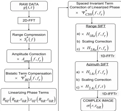
Frequency Domain Focusing Algorithm ... 89 Figure 42: Optical Image (Google Map) of Niederweidbach ... 90 Figure 43: Stationary Receiver Configuration ... 92 Figure 44: Block Diagram of Focusing Algorithm (Stationary Receiver
Configurations) ... 95 Figure 45: Focusing Result of Stationary Receiver Experiment (Dreis-Tiefenbach)
using Frequency Domain Algorithm... 99 Figure 46: Focusing Result of Stationary Receiver Experiment (Dreis-Tiefenbach)
using Back Projection Algorithm ... 99 Figure 47: Comparison of some parts of the scene (Dreis-Tiefenbach) ... 100 Figure 48: Histogram of the Normalized Amplitude of the Time and Frequency
Domain Processed Images ... 101 Figure 49: Interferometric Phase of the Time and Frequency Domain Images and its
Overlap on the Intensity Image ... 101 Figure 50: Focusing Result of Stationary Receiver Experiment (Koblenz) using the
Frequency Domain Algorithm ... 102 Figure 51: Focusing Result of Stationary Receiver Experiment (Koblenz) using
Back Projection Algorithm ... 102 Figure 52: Comparison of a part of the scene (Koblenz) ... 103 Figure 53: Histogram of the Normalized Amplitude of the Time and Frequency
Domain Processed Images ... 103 Figure 54: Interferometric Phase of the Time and Frequency Domain Images and its
Overlap on the Intensity Image ... 104 Figure 55: Interferogram of the Scene (Dreis-Tiefenbach) – Using Frequency
Domain Algorithm ... 105 Figure 56: Interferogram of the Scene (Dreis-Tiefenbach) – Using Time Domain
Processing Approach... 105 Figure 57: Interferometric Phase Overlaid on the Radar Intensity Image
(Dreis-Tiefenbach) ... 106 Figure 58: Differential Interferogram ... 106
List of Tables
Table 1: Parameters for Hybrid Configuration ... 38
Table 2: Parameters for Tandem Configuration ... 54
Table 3: Parameters for Translational Invariant Configuration ... 57
Table 4: Quality Parameters for Focused Point Target using L1T ... 63
Table 5: Quality Parameters for Focused Point Target using L1R ... 66
Table 6: Quality Parameters for Focused Point Target using L2T ... 67
Table 7: Quality Parameters for Focused Point Target using L2R ... 69
Table 8: Bistatic Airborne Experiment (Azimuth Invariant TI Configuration) ... 82
Table 9: Hybrid Bistatic SAR Experiment (Pommersfelden, Germany) ... 85
List of Acronyms
AER-II Airborne Experimental Radar AIC Azimuth Invariant Configurations AVC Azimuth Variant Configurations
BPTRS Bistatic Point Target Reference Spectrum
COSMO Constellation of small Satellites for Mediterranean basin Observation CSA Canadian Space Agency
CNES Centre National d’Etudes Spatiales (French Space Agency) DEM Digital Elevation Model
DPLL Digital Phase Locked Loop
DLR Deutsches Zentrum für Luft und Raumfahrt (German Space Agency) EM Electromagnetic Radiations
ERS European Remote Sensing ESA European Space Agency
FGAN Forschungsgesellschaft für Angewandte Naturwissenschaften (Research Establishment for Applied Natural Sciences)
FFT Fast Fourier Transformation
GMES Global Monitoring for Environment and Security GPS Global Positioning System
IDL Interactive Data Language
IFFT Inverse Fast Fourier Transformation INS Inertial Navigation System
InSAR Interferometric Synthetic Aperture Radar IRW Impulse Response Width
ISLR Integrated Side Lobe Ratio
JERS Japan Earth Remote Sensing Satellite LBF Loffeld’s Bistatic Formula
NASA National Aeronautics and Space Administration NASDA National Space Development Agency
NRL Naval Research Laboratory
ONERA Office National d'Études et de Recherches AÉrospatiales (French Aero-space Research Center)
PAMIR Phased Array Multifunctional Imaging Radar
PCA Point of Closest Approach
PRF Pulse Repetition Frequency PRI Pulse Repetition Interval PSLR Peak Side Lobe Ratio PSP Point of Stationary Phase PT Point Target
QinetiQ British Defense Technology Company RADAR Radio Detection and Ranging
RAR Real Aperture Radar
RCMC Range Cell Migration Correction SAR Synthetic Aperture Radar
SABRINA SAR Bistatic fixed Receiver for Interferometric Applications SIFT Scaled Inverse Fourier Transformation
SIR SAR Imaging Radar
SLAR Side-Looking Aperture Radar SNR Signal to Noise Ratio
TBP Time Bandwidth Product
TI Translational Invariant
TIRA Tracking and Imaging Radar
List of Symbols
range
Slant range resolution
azimuth
Azimuth resolution
0
c Velocity of light (i.e. 3 10 8m s/ )
r
B Transmitted signal bandwidth
Azimuth time (Slow time)
t Range time (Fast time)
0
t Two ways signal traveling time
( )
R
R Receiver’s slant range
( )
T
R Transmitter’s slant range
0R
Azimuth time when receiver is at closest distance from the point target 0T
Azimuth time when transmitter is at closest distance from the point target 0R
R Slant range when receiver is at closest distance from the point target 0T
R Slant range when transmitter is at closest distance from the point target
R
v Receiver’s velocity
T
v Transmitter’s velocity
0R, 0R
P R Point target in receiver’s coordinates
0Rd Distance between transmitter and receiver at receiver’s PCA 0
a Difference between transmitter and receiver azimuth times at PCA 2
a Ratio of transmitter and receiver slant ranges at PCA 0
f Carrier frequency
f Range frequency f Azimuth frequency
T
f Weighted azimuth transmitter frequency
R
f Weighted azimuth receiver frequency ( )
l
s t Transmitted signal ( )
l
g t Received signal in time domain
R0R, 0R
Backscattering coefficient
c
Azimuth time window with center time c ( )
l
G f Received signal in frequency domain
B
Bistatic phase term
R
Receiver’s phase term
T
Transmitter’s phase term
S
Intermediate phase term Weighting factor
T
Individual PSP of transmitter
R
Individual PSP of receiver
Common point of stationary phase
QM
Quasi monostatic phase term
BD
Bistatic deformation phase term
DCt
f Doppler centroid transmitter
DCr
f Doppler centroid receiver
SQt
Squint angle transmitter
SQr
Squint angle receiver
T
E Transmitter range rate error
R
E Receiver range rate error 1T
2T
L Second validity constraint of transmitter 2R
L Second validity constraint of receiver Upper limit of weighting factor Lower limit of weighting factor
CS
Complete scene phase term
LCS
Linearized complete scene phase term 0
CS
Space invariant complete scene phase term
_ CS Ra
Range variant complete scene phase term
_ CS Az
Azimuth variant complete scene phase term
Ra
A Range shift term
Ra
B Range scaling term
Az
A Azimuth shift term
Az
1 Introduction and Historical Background
A significant contribution to the evolution of radar technology was made by a German physicist, Heinrich Hertz (1857-1894). As a result of his experiments, he witnessed the reflection of electromagnetic waves by metallic objects and successfully proved the generation and detection of radio waves. A Scottish physicist, James Clerk Maxwell (1831-1879) had also predicted the existence of electromagnetic waves and his theoreti-cal investigations led to the formation of the renowned Maxwell’s equations. Guglielmo Marconi, the pioneer of wireless communication, was a keen promoter of practical radio systems. In 1904, a German engineer, Christian Hülsmeyer gave a public demonstration regarding the detection of ships in fog and poor visibility scenarios using radio waves. He was the first one to build a simple ship detection device called the ‘Telemobiloscope’ but the naval authorities of that time failed to recognize its worth (registered as patent Nr. 165546).
Before the Second World War, parallel efforts for the development of radar systems were initiated by the British, the Germans, the French, the Soviets, the Japanese and the Americans. In USA, most of the earlier developments were made by the Naval Research Laboratory (NRL). In 1930s, both United Kingdom and Germany were successful in demonstrating the tracking of aircrafts using short pulse ranging measurements. In 1937, first operational radar system was developed in United Kingdom by Robert Wat-son-Watt and his companions. Their work proved useful during the Second World War to track the aircrafts across Europe.
The word RADAR is an acronym suggested by the U.S. Navy in 1940. It stands for RAdio Detection And Ranging. Since the Second World War, it has been used for ob-servation purposes. It is a magnificent tool to detect objects and measure their range (distance) and speed. Later the technological developments over decades made it possi-ble to construct images of the Earth’s surface, using Synthetic Aperture Radar (SAR) principles.
1.1 Synthetic Aperture Radar
Imaging active sensors operating in the microwave region of the electromagnetic (EM) spectrum are usually referred to as the Real Aperture Radar (RAR). They offer day and night including all weather imaging along with continuous and global monitoring of the Earth’s surface. The main limitation of these sensors is the poor cross range resolution, which is directly proportional to the radiated wavelength and slant range from the
sen-that if a satellite is operating at a point, say, hundreds of kilometers of altitude from the surface, it would require an antenna of length from several hundred meters to kilometers depending on the wavelength of transmitted signal in order to achieve a resolution in meters. Such a long antenna is practically not feasible. This limitation was overcome using the concept of SAR, where azimuth resolution is independent of the sensor’s alti-tude (see section 1.2.1).
SAR usually referred as the imaging radar, utilizes the concept of creating a very long antenna aperture with the help of signal processing techniques. SAR principle was first registered as a patent in 1954 by Carl A. Wiley of the Goodyear Aerospace Corporation, titled “Pulsed Doppler Radar Method and Means” (US Patent Nr. 3.196.436). He used the Doppler information to increase the azimuth resolution of the Side Looking Aper-ture Radar (SLAR). The first satellite carrying a SAR sensor was launched in 1978 by NASA for remote sensing applications. The data collected in a 100 days mission of Seasat-A showed that SAR is a wonderful tool for measuring the Earth’s surface charac-teristics. It is a coherent system which retains both amplitude and phase of the backscat-tered echo signals. It combines the echo signals from each pulse to produce a high reso-lution image of the terrain as compared to that obtained by a much larger antenna. SAR technology can be used with aircrafts (Airborne SAR), satellites (Satel-lite/Spaceborne SAR) or a combination of both aircrafts and satellites (Hybrid SAR). The data collected by SAR sensors is called raw data. Important information lies in the phase of this raw data and with appropriate processing algorithm it can be transformed into a focused SAR image. More details of SAR processing will be provided in the next chapters.
1.1.1 SAR Advantages and Applications
SAR, as an active microwave sensor is capable of monitoring continuously the proper-ties of the geophysical parameters of the Earth’s surface. It opens new horizons for the remote sensing and global monitoring of the Earth’s natural resources. Being an active sensor, it transmits EM radiations in the microwave region of the EM spectrum. There-fore, it is independent of sunlight. Thus, allowing continuous day and night operations. Spaceborne SAR sensors operate generally between 1-10 GHz (3-30 cm) of microwave region. It is possible to choose appropriate wavelength of the transmitted signal which offers less attenuation due to clouds, fog and precipitation. Thus, it is suitable for all weather conditions. It offers good resolution at remote distances, large area coverage and rapid data acquisition throughout the year. It has made possible to continuously monitor and gain information about the ocean currents, iceberg movements, oil films on ocean waters, surface mapping, geological structures, soil moisture, soil erosion, floods,
the SAR sensors reflect differently from different materials and thus can provide a bet-ter discrimination of the surface features. It is possible to acquire images of areas with backscattering characteristics of EM radiations and it also offers better resolution as compared to the conventional radar systems. SAR is widely used in the applications for remote sensing and mapping of the surface of the Earth and of the other planets.
1.2 SAR Principle
The basic principle of SAR is to synthesize a longer antenna aperture with the help of spaceborne or airborne platform to achieve better azimuth resolution. As the platform moves along the trajectory, it transmits pulses at regular azimuth time intervals. The reflected echoes are linear superposition of the received signals of each point target within the antenna’s foot print and are coherently recorded and processed. This post processing technique creates a larger synthetic aperture as compared to the physical antenna length and hence generates high resolution SAR images. The length of the flight path during which point target remains illuminated corresponds to the synthetic aperture length as shown in Figure 1. In monostatic SAR, same sensor is used for the transmission and reception of radar pulses. The range of the point target varies with the motion of platform. It decreases and reaches its minimum value at point of closest ap-proach (shortest distance between point target and platform trajectory) and then increas-es as the platform movincreas-es. Hence, the range history in this case, takincreas-es the shape of a hy-perbola.
Flight Direction
Synthetic Aperture Length
Figure 1: Synthetic Aperture Length
Pulses are emitted by the antenna which illuminates the Earth’s surface. The ground area illuminated by the pulses is called the antenna’s footprint as shown in Figure 2. The illuminated ground area may consist of large number of small point targets. Each point target reflects the signal back to the antenna according to its own backscattering strength. The along track motion of the sensor is called azimuth direction. The slant
range represents the distance from the antenna to the point target and is a measure of the roundtrip propagation delay of the radar pulses.
Flight Direction Azimu th Slan t Range Height Illuminated Swath Antenna Footprint
Figure 2: SAR Principle
The reflected signal is basically the superposition of the back scattered signals from all point targets in the antenna footprint. The received signal is demodulated from its car-rier signal and is converted into a baseband signal. It is then recorded as two dimen-sional raw data. This raw data is processed using a focusing algorithm. The focused image is superposition of impulse responses from all point targets.
1.2.1 SAR Resolution
The pulse length used in the practical systems is long enough to obtain a good tion. Pulse compression technique is used to obtain narrow pulses and hence fine resolu-tion in the range direcresolu-tion. Slant range resoluresolu-tion is defined as:
0 2 range r c B (1.1)
It depends on the transmitted pulse bandwidth Br and the velocity of light c0. It does not depend on the physical antenna length.
In azimuth direction better resolution is obtained by using the fact that different scatter-ers in a radar beam reflect energy with a different Doppler shift. Using this Doppler shift an aperture of several kilometers can be synthesized with an improved azimuth resolution. In stripmap SAR mode (explained in section 1.4), the azimuth resolution is given as:
2
azimuth L
The azimuth resolution is equal to half of the physical antenna length L and it is inde-pendent of the slant range. The azimuth resolution is also called along track or cross range resolution.
1.3 Bistatic SAR
Bistatic SAR is a promising and useful advancement of monostatic SAR systems. In general bistatic SAR configurations, transmitter and receiver are located on different platforms, thus offering considerable flexibility in designing bistatic SAR missions us-ing a combination of spaceborne, airborne or stationary ground-based platforms. Classi-fication of objects in bistatic SAR images is improved and additional information of scene is obtained using bistatic SAR systems. Another advantage of bistatic SAR is to use one transmitter with several passive receivers. In a hostile environment, it is more appropriate to use an active transmitter far from the scene with passive receivers located closer to the scene. As the receiver is passive, therefore it can not be easily detected. In bistatic SAR images, dihedral and polyhedral effects are reduced especially in the urban areas, due to decrease in multipath scattering. They can image in flight direction and backwards.
Despite all these advantages, bistatic SAR configurations offer many technical chal-lenges. Major challenges are time synchronization of transmitter and receiver platforms and motion compensation. Bistatic SAR processing itself is a non trivial task. Ad-vancements in navigation and communication technologies made it possible to address some of these issues. European radar research institutes like German space agency (DLR), Fraunhofer institute for high frequency physics and radar techniques-FHR (for-mer FGAN), ONERA and QinetiQ have made remarkable progress in the spaceborne/airborne bistatic SAR experiments [19]-[22].
1.4 SAR Modes
SAR can be operated in different modes. The basic operating modes are stripmap, scan and spotlight. In stripmap SAR mode, antenna points to a fixed direction with respect to the flight path and the antenna’s footprint sweeps a strip on the ground during sensor’s flight as shown in Figure 3. It enables continuous imaging. The azimuth resolution de-pends on the length of antenna. The image dimension is limited in range but not in azi-muth.
Flight Direction
Figure 3: Stripmap SAR Mode
In scan SAR mode, a wider range swath is imaged as compared to the stripmap SAR. During data intake, antenna is scanned in range several times which is achieved by peri-odically shifting the antenna beam to neighboring sub swaths, as shown in Figure 4. SAR operates continuously but only a portion of synthetic aperture is available for each target in sub swath. The azimuth resolution is therefore decreased as compared to the stripmap mode due to wide swath. This mode provides a trade off between wider range swath dimensions and poor azimuth resolution.
Flight Direction
Figure 4: Scan SAR Mode
The spotlight mode is used to image some area of interest or spot on the ground as shown in Figure 5. The radar antenna is steered to illuminate the spot during the overall data acquisition time. It does not offer continuous imaging but an improved azimuth resolution due to increase in angular extent of illumination of the spot. In this mode, beam is steered backward as the sensor moves forward thus creating an effect of a wider antenna beam. The number of received backscattered echoes by each target in the scene increases significantly as compared to the stripmap mode, thus improving azimuth reso-lution. This mode provides a trade off between better azimuth resolution and limited
Flight Direction
Figure 5: Spotlight SAR Mode
The sliding SAR mode is a combination of stripmap and spotlight as shown in Figure 6. In this mode, antenna’s footprint slides over the Earth’s surface with accelerated or re-duced footprint velocity with respect to the platform’s velocity (aircraft or satellite). The looking direction of the antenna beam can be forward or backward. This mode offers a balance between azimuth scene extent and resolution.
Figure 6: Sliding SAR Mode
In the inverse SAR mode, SAR sensor is stationary and target is moving which can be used to track aircrafts and satellites from a ground base radar system. In this mode movement of targets generates the synthetic antenna.
The Interferometric SAR (InSAR) provides an opportunity for obtaining 3D SAR imag-es. They are obtained by combining two or more coherent images of the same scene taken by two antennas with slightly different observation angles and exploring the phase difference among them. It is also referred to as the phase interferogram. If the two an-tennas are separated along range and are perpendicular to the flight track, they are called across track InSAR. Across track InSAR configurations may consist of a system with
interferometer) or a system with a single antenna having two time separated passes over the same scene (two pass interferometer).
1.5 Spaceborne SAR Missions
The launch of Seasat in 1978 by NASA has opened a new era in the remote sensing. It was the first civilian spaceborne SAR. It operated at L-band. Later during 1990s, the European Space Agency (ESA), the National Space Development Agency (NASDA) of Japan and the Canadian Space Agency (CSA) decided to join NASA for developing SAR systems for global monitoring of the Earth’s natural resources. In March 1991, the Soviet Union launched S-band satellite named ALMAZ. Followed by the launch of ERS-1 (European Remote Sensing Satellite) which was a C-band SAR system. The im-age showed in Figure 7 is captured by ERS-1 (SAR) of Malaspina glacier in Alaska in July 1992. In 1995, ERS-2 was launched which was identical to the ERS-1. Both satel-lites shared the same orbit with the time delay of one day at an altitude of almost 800 km. Such constellations helped to carry out the interferometric TanDEM-X mission.
Figure 7: ERS-1 (SAR) Image © ESA
Another successful mission was C/X band spaceborne SAR Imaging Radar (SIR) launched in 1994 on a space shuttle. It has recorded the SAR data in L, C and X band. An image of Petra region (Jordan) acquired by SIR-C/X (SAR) in April 1994 is shown in Figure 8. It was a joint mission of the German, Italian and American space agencies.
Figure 8: SIR-C/X (SAR) Image [Courtesy NASA/JPL-Caltech]
The Japanese Earth Remote Sensing (JERS-1) satellite was launched in 1992. It was an L-band SAR system for the observation of geological changes and environmental moni-toring. The CSA launched RadarSat-1 in 1995. It was a C-band SAR system with the main purpose for daily monitoring of the Arctic glaciers and icebergs. It was capable of providing SAR images with a spatial resolution of 10m. RadarSat-2 was launched in 2007 which was able to provide a spatial resolution of 3m. COSMO-SkyMed (Constel-lation Of small Satellites for Mediterranean basin Observation) is an Earth observation Italian satellite system with X-band SAR sensors used for the global monitoring and coverage of the Earth’s surface. The first COSMO-SkyMed satellite was launched in June 2007, followed by the launch of a second satellite in December 2007 and still an-other in October 2008. SAR-Lupe is a German satellite system of five identical satellites controlled by a ground station. It uses X-band and operates in spotlight and stripmap modes. Its first satellite was launched in December 2006 and the last one was launched in July 2008. Another, TerraSAR-X, a German Earth observation satellite was launched in 2007. Its data is available both for the scientific purposes and for the commercial use. It has ability to get high resolution Earth images and has been designed to carry out its tasks for five years. It can acquire radar data in stripmap, spotlight and scan SAR modes. It was followed by the launch of another satellite, TanDEM-X in June 2010. Both satellites work in pair to generate a global high resolution Digital Elevation Model (DEM) of the Earth.
The interferometric cartwheel was proposed by D. Massonnet [65] at a research pro-gram of the French Space Agency (CNES). It consists of multistatic SAR configuration of three passive micro satellites working with an active SAR satellite. Its purpose is to build a cost effective system which can produce an accurate DEM. The advantage of this concept is stable, horizontal and vertical baselines due to orbital configuration. Sta-ble baselines are very important in the SAR interferometry as a small error in baseline
improve the final image resolution and can produce along and across track interferomet-ric data.
Sentinel-1 is a future European radar observation satellite system (Figure 9). It is a C-band SAR mission expected to launch in 2013. Its data would be used by the Global Monitoring for Environment and Security (GMES) and ESA for land and ocean obser-vations.
Figure 9: Sentinel-1 Satellite © ESA
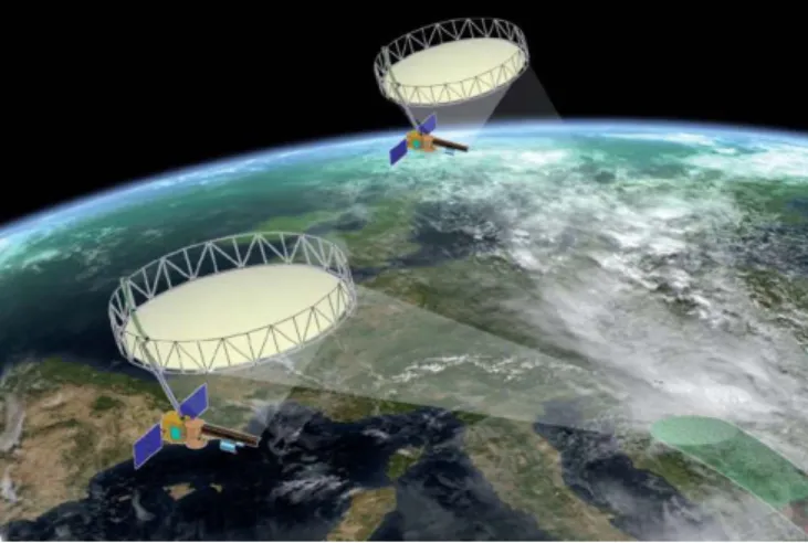
Tandem-L is a proposed future satellite (Figure 10) for L-band interferometric and polarimetric SAR missions, used for global monitoring of forestation, forest biomass changes, earthquakes, volcanic activities, ice cover and mass changes, flooding etc.
Figure 10: Tandem-L Satellite © DLR & ESA
1.6 SAR Processing
Different processing algorithms have been proposed to focus SAR data. Algorithms developed in the time domain to focus SAR data are more precise but computationally
efficient and easy to implement. Therefore, frequency domain algorithms are mostly preferred [1]-[55].
Bistatic SAR processing is more complicated than the monostatic SAR. Bistatic SAR data can be azimuth invariant as both transmitter and receiver can have different motion trajectories. In monostatic SAR, range history has a hyperbolic shape. Where as, in bistatic SAR range history is more complicated, as it is the sum of transmitter and re-ceiver ranges. The sum of two hyperbolic range histories of the transmitter and rere-ceiver, results in a double square root term in the bistatic range history. It has the shape of flat-top hyperbola. It is not possible to focus the bistatic SAR data using monostatic SAR algorithms. They must be modified to handle bistatic SAR configurations.
Back projection algorithm is implemented in the time domain for SAR data processing. Its computational complexities can be reduced using fast back projection processing techniques. A frequency domain bistatic SAR processing approach was proposed by Prof. Rocca and his team at Milan Polytechnic University. They used a technique which was already available for monostatic SAR processing. In this preprocessing technique [14], Dip Move Out operator (also called as ‘smile’ operator) is used to convert bistatic SAR data into monostatic for constant offset configuration. Later, it has been extended to general bistatic SAR configurations. Prof. Ender and his team at Fraunhofer-FHR have proposed Omega–k algorithm for bistatic SAR processing for Translational Invari-ant (TI) configurations (transmitter and receiver moving parallel to each other with con-stant velocities and offset) and tandem configurations (transmitter and receiver follow-ing each other on a sfollow-ingle path with constant offset) [20], [26]. They have also used back projection and range Doppler processors for real bistatic SAR data processing [19].
Prof. Bamler and his team at DLR (German Aerospace Center) proposed a numerical transfer function for TI configurations [34]. There focusing algorithm replaces the ana-lytical SAR transfer function with numerical equivalent and are able to handle azimuth invariant and squinted configurations. I. Cumming, F. Wong and Y. Neo derived 2D point target reference spectrum based on extended nonlinear chirp scaling algorithm [41]-[42], and a method of series reversion for the processing of general bistatic SAR configurations [43].
Prof. Loffeld at the University of Siegen derived a Bistatic Point Target Reference Spectrum (BPTRS) known as Loffeld Bistatic Formula (LBF) for general bistatic SAR configurations [1]-[2], [6]-[8]. It consists of the quasi monostatic phase term and bistatic deformation term. A Scaled Inverse Fourier Transformation (SIFT) is used to process bistatic SAR data for general configurations [3], [5], [8]. It works well for those
config-focus in azimuth. Dr. Wang came up with the idea of extended Loffeld’s bistatic formu-la [46]-[50] with unequal azimuth contribution of transmitter and receiver phases, by using the Time Bandwidth Product (TBP). My work is also based on the unequal azi-muth contribution of transmitter and receiver phase terms for bistatic SAR configura-tions by using a weighting factor derived by minimizing the square difference between common and individual points of stationary phases of transmitter and receiver [53]-[57]. More details are given in the next chapters.
1.7 Structure of the Thesis
This thesis is structured as follows:
First chapter is based on the overview of synthetic aperture radar. Evolution of SAR over years, its working principle, its modes, spaceborne missions and processing tech-niques are discussed in Chapter 1.
Bistatic point target reference spectrum based on the Loffeld’s bistatic formula is de-rived in Chapter 2. It presents the bistatic signal model and point target impulse re-sponse function. It is based on different azimuth contributions of transmitter and receiv-er phase treceiv-erms.
Four validity constraints based on different azimuth contributions of transmitter and receiver phase terms are derived in Chapter 3. They were used to find different weighting to azimuth contribution of transmitter and receiver phases.
Focusing of the complete scene for different bistatic SAR configurations are discussed in Chapter 4. A frequency domain processing algorithm is implemented using a SIFT and is applied to focus real bistatic SAR data.
Stationary receiver configurations are considered in Chapter 5. A BPTRS is derived and based on it an appropriate frequency domain processing algorithm is implemented. This algorithm is used to focus the real bistatic SAR data obtained during the stationary receiver experiments conducted at the University of Siegen.
2 Bistatic Point Target Reference Spectrum
2.1 Introduction
An approximated BPTRS is derived in [1]. This frequency domain processing approach called LBF provides an analytical solution for focusing different bistatic SAR configu-rations. The method of stationary phase has been used in its derivations. The phase terms are expanded using Taylor’s series around the individual stationary points of the transmitter and receiver.
This chapter contributes towards the theoretical understanding of the bistatic SAR sig-nal model. It begins with the description of general bistatic SAR geometry. Using this geometry, a bistatic signal model is derived. Later, an analytical BPTRS based on LBF is derived, assuming different azimuth contributions of the transmitter and receiver phases. The transmitter and receiver phases are weighted differently based on their con-tributions towards the bistatic phase history.
2.2 Bistatic SAR Geometry
In bistatic SAR, transmitter and receiver are located on different carrier platforms. A general bistatic SAR configuration offers a complex geometry, with the transmitter and receiver moving in different directions with different velocities. The bistatic SAR con-figurations can be used in a variety of constellations between the transmitter and receiv-er e.g. using two airborne/spaceborne platforms as transmittreceiv-er and receivreceiv-er, spaceborne platform as transmitter with an airborne platform as receiver, or a moving transmitter platform with a stationary receiver, etc. The transmitter and receiver are separated in space but they must be synchronized by using some communication channel or by direct reception of the transmitted signal by the receiving unit.
Transmitter’s Path Receiver’s Path T v R v R R R0T , PT R T R 0R R Z Y
The bistatic SAR geometry of a general configuration is shown in Figure 11. We sup-pose a flat Earth model and a Cartesian coordinate system. The platforms are flying along y-axis and their heights are along z-axis. The imaged scene is in the xy-plane. Here we assume that the transmitter and the receiver are moving with different veloci-ties along non parallel tracks. The velocity vectors of the transmitter and receiver are denoted by vT and vR. The time along the flight axis is called the azimuth time . The
distances of the transmitter and the receiver from the point target are referred as the slant ranges and are denoted by RT
and RR
respectively. For simplicity, we have considered only one point target and is represented in receiver’s coordinates
0R, 0R
P R . The azimuth time when transmitter (or receiver) is at the closest distance from the point target, is also referred as the time at Point of Closest Approach (PCA) of the transmitter (or receiver) and is denoted as 0T ( or 0R). The slant ranges at PCA of the transmitter and receiver are denoted by R0T and R0R respectively.
2.3 Bistatic SAR Signal Model
In bistatic SAR geometry, the slant range histories of transmitter and receiver can either be expressed in transmitter related or receiver related coordinates. In our approach, we specify the position of a PT at time instant 0R, when it is at PCA of the receiver at a
slant range R0R. Similarly, transmitter related coordinates can also be used for general bistatic SAR configurations. The choice of coordinates also depends on the bistatic SAR configuration or its application. For example, in case of a stationary transmitter (or re-ceiver) and moving receiver (or transmitter) configurations, it is more appropriate to express the bistatic slant range histories in terms of the moving platform.
In bistatic SAR we have two carrier platforms. The angle between the lines joining the transmitter and receiver with the point target, keeping the point target in the center, is called the bistatic angle [shown in Figure 12]. The line joining transmitter and receiver is called the baseline and is denoted by d
.Transmi tter Path Rece iver Path Y
R R
d T
R Basel ine Bistatic Angle Point TargetWe assume that both the platforms are moving with constant velocities along straight flight path. The slant range vectors of the receiver and transmitter at any azimuth time instant can be written as:
2
2
20 0 0 0 0 0
, , , ,
R R R R R R R R R
R R R R v (2.1)
From Figure 13, it can be seen that the slant range R0R at PCA of the receiver is per-pendicular to the velocity vector vR.
Point Target
R R 0R 0 ()RR v 0R R R vFigure 13: Slant Range Relationship
Similarly, the slant range equation for the transmitter will take the form as:
2
2
20 0 0 0 0 0
, , , ,
T R R T T R R T T
R R R R v (2.2)
It depends on the azimuth time and velocity of the platform. The received signal is rec-orded coherently in range and azimuth directions. The bistatic slant range is sum of the transmitter and receiver slant ranges, which is in fact sum of two hyperbolic ranges. It is given as:
, 0 , 0
, 0 , 0
, 0 , 0
B R R T R R R R R
R R R R R R (2.3)
The signal propagation time is denoted by t0 and can be written as:
0 0
0 0
0 0 0 0 , , , , , , T R R R R R R R R R R R t R c (2.4)The transmitter and the receiver should be synchronized. The phase stability of the local oscillator is important to have well focused images. For bistatic SAR configurations with large and rapidly changing baselines, synchronization of transmitter and receiver is not a trivial task and it may result in poorly focused images.
2.4 Bistatic Point Target Response
The transmitter emits pulses at regular Pulse Repetition Interval (PRI) during its flight. These pulses are up converted to a certain carrier frequency f0 before transmission. The transmitted signal is usually a linear frequency modulated signal (e.g. chirp signal) with instantaneous frequency as a linear function of time. The received echo is down con-verted and sampled with a sampling rate greater than signal bandwidth Br to avoid
ali-asing [83]. The received signal is considered as a time delayed replica of the transmitted signal. The received signal after demodulation to a base band signal for a point target response is given as:
2 0 00 0 0 0 0
, , , , j f t
l R R R R c l
g t R R w s t t e (2.5)
Where,
R0R,0R
is the backscattering coefficient. It provides information about the brightness of a point target. w
c
is a rectangular window with center time c.
0
l
s t t is the delayed transmitted signal.
2.5 Bistatic Point Target Reference Spectrum
The received signal in equation (2.5) is represented in the time domain. After perform-ing the Fourier transformation over the range time t and azimuth time , we get the point target spectrum in range frequency f and azimuth frequency f domain.
After performing the Fourier transformation over range time t, on the received signal given in equation (2.5), we get:
2 0 00 0 0 0
, , , , j f f t
l R R R R c l
G f R R w S f e (2.6)
We substitute t0 from equation (2.4) and perform the Fourier transformation over azi-muth time . We obtain:
0 0 0 0 0 0 0 0 0 0 2 , , , , , , , , T R R R R R l R R R R l f f j R R R R f c c G f f R R S f w e d
(2.7)Where, G f fl
,
is the received signal spectrum in frequency domain. The phase term in equation (2.7) is called as the bistatic phase term and is denoted by:
0
0 0 0 0 0 2 , , , , B f fc RT R R R RR R R R f (2.8) The bistatic phase depends on the range and azimuth frequencies and the slant range histories of the transmitter and receiver. As both transmitter and receiver contribute to the bistatic phase, we can express it as the sum of transmitter and receiver phase terms.
0 0 0 0 0 0 0 0 2 , , 2 , , T T R R T R R R R R f f R R f c f f R R f c (2.9)The weighted azimuth frequencies of the transmitter and receiver are defined as:
(2 )
;
2 2
T R
f f f f (2.10)
Here, is the weighting factor which represents the unequal azimuth contribution of the transmitter and the receiver phases. In [1], equal azimuth contribution of the trans-mitter and receiver phases is considered i.e. 1. It works well for those bistatic SAR configurations where the transmitter and receiver both contribute equally towards the bistatic phase. But in certain configurations like hybrid configurations where the trans-mitter and receiver have large differences in the altitudes and velocities, we assume dif-ferent azimuth contributions of the transmitter and receiver in the bistatic phase. An analytical expression for the weighting factor is derived in the next section. In every case, fT fR f is satisfied.
The Method of Stationary Phase (MSP) has been used in the derivation of LBF [1]. The phase term in equation (2.7) oscillates very fast and most of the contribution of the inte-gral comes from the vicinity of the stationary point. At the stationary point, the gradient of a function becomes zero [83]. The phase terms of the transmitter and receiver are expanded around their individual Points of Stationary Phases (PSP) , T R using the Taylor’s expansion. The second order Taylor’s expansion of the transmitter and receiver phases is given as:
2 2 1 ... 2 1 ... 2 T T T T T T T T T R R R R R R R R R (2.11)0 ; 0 T R T R d d d d (2.12) Simplifying equation (2.11) using equation (2.12), the bistatic phase term can be written as:
1
2 1
2 ...2 2
B T T R R T T T R R R
(2.13)
Substituting equation (2.13) into (2.7), and taking constant terms outside the integral, we get the following expression:
2 2 ( ) ( ) 0 0 0 0 1 2 , , , , T T R R T T T R R R j l R R R R l j c G f f R R S f e w e d
(2.14)The phase term inside the integral is sum of two quadratic terms. As the sum of two quadratic terms remains quadratic, so they can be regrouped and expanded around a common PSP. Let the phase terms of the integral be denoted by:
2
2S T T T R R R
(2.15)
The common PSP is obtained as follows:
0 T T T R R R S T T R R d d (2.16) The phase term given in equation (2.15) is expanded using the second order Taylor’s expansion and we get:
1
2 ...2
S S S
(2.17)
Using equations (2.15) and (2.16), we can simplify equation (2.17) as:
T
T R
R
2
2 S R T T T R R T T R R (2.18) The phase term of equation (2.18) is substituted into (2.14). After simplifications, we obtain the BPTRS as follows:
0 0 0 0 4 2 2 , , , , BD QM l R R R R l cb T T R R j j j G f f R R S f w e e e (2.19)The first phase term in equation (2.19) is called as the Quasi Monostatic (QM) term and the second term is called as the Bistatic Deformation (BD) term. These phase terms are expressed as follows:
2 ( ) ( ) ; T T R R QM T T R R BD T R T T R R (2.20) The transmitter and the receiver phase terms can be simplified mathematically. The ex-panded derivations of these results are given in Appendix A. The second order deriva-tives of the phase terms at the individual PSP of the transmitter and receiver are simpli-fied as:
2 0 3 2 2 0 0 0 2 0 3 2 2 0 0 0 sgn 2 , sgn 2 , T T T T T R R R R R f f v F f f c R f f f f v F f f c R f f (2.21)Where, ,F FT R represent frequency histories and are given as:
2 2 2 2 0 0 2 2 2 2 2 0 0 2 , 4 (2 ) , 4 T T R R f c F f f f f v f c F f f f f v (2.22)The individual PSP of the transmitter and the receiver are obtained as below:
0 0 0 0 2 1 2 0 0 0 0 2 1 2 sgn 2 , sgn (2 ) 2 , T T T T T R R R R R R f f f c v F f f R f f f c v F f f (2.23)The common PSP is derived as follows:
2 3 2 2 3 2 0 0 2 0 0 2 0 2 3 2 2 3 2 2 (2 ) 2 T T R R R R R T R T T R R v F a a v F c a R f F F v F a v F (2.24)Here a a0, 2 are called the system parameters. a0 is the azimuth time difference of the transmitter and receiver at PCA. Whereas, a2 is the slant range ratio of the transmitter and receiver at PCA and are given as:
0 0 0 0 2 0 ; T T R R R a a R (2.25)
The QM and BD phase terms given in equation (2.20) are simplified as follows:
0 0 1 2 1 2 0 0 2 0 2 2 3 2 3 2 0 2 3 2 2 2 3 2 0 0 0 2 2 2 2 0 0 0 2 0 2 2 1 2 1 2 2 sgn 2 sgn 2 2 sgn( ) 2 R QM R R T T R R T BD R T T R R T R R T R T R R f f f a F a F c f f v v F F R c f f F v a v F v f c R f f a v a v v F F (2.26)The two dimensional BPTRS based on the LBF for unequal azimuth contribution of the transmitter and receiver phase terms is given in equation (2.19), can be simplified using the equations (2.21) - (2.26). This BPTRS is essential for the development of the bistatic SAR processing algorithm.
2.6 Optimum Weighting Factor
In the final expression of BPTRS, all parameters except the weighting factor are known. The next step is to derive an analytical expression for the weighting factor. We know that the MSP has been used in the derivation of LBF [1]. It is only applicable if the common PSP is located in the vicinity of the individual PSPs of the transmitter
T
and the receiver R. Also, the individual PSPs of transmitter and receiver should not be too far apart.
Based on the above mentioned facts, we come up with an idea that the weighting factor can be obtained by minimizing the square difference between the individual PSPs of the transmitter and receiver, and is given as:
2 0T R
d
d
(2.27) Simplifying the above equation, we get:
Derivation of individual PSPs of the transmitter and receiver with respect to the weighting factor can be obtained using equation (2.23) as:
0 0 2 0 0 0 2 0 2 2 T T T R R R f c R d d v f f f c R d d v f f (2.29)The frequency histories of the transmitter and receiver given in equation (2.22) are ap-proximated as:
2 0 2 0 , , T R F f f f f F f f f f (2.30)Substituting equations (2.23) and (2.29) into (2.28), we get:
0 0 0 0 0 2 0 2 0 0 0 0 0 0 2 2 0 0 (2 ) 2 2 2 0 2 2 T R T R T R T R T R f c R f c R f f f f v v f c R f c R f f f f v v (2.31)After simplifying the above equation, we get weighting factor as follows:
2 2 0 0 0 0 2 2 2 0 0 0 0 2 2 0 0 2 2 0 0 2 2 2 1 R T R R T R R T R T R R T f f v v f c R a f c R v R v v f f a v f f v f c R a v v (2.32)The above equation shows that the weighting factor depends upon the range and az-imuth frequencies, the platform velocities, slant ranges and azaz-imuth time of the trans-mitter and receiver at PCA.
2.6.1 Simulation Results
An analytical solution for the weighting factor is obtained by using the fact that MSP can only remain valid if we have a single PSP. Therefore, the difference between the individual PSPs of the transmitter and receiver should remain as small as possible, i.e.
Table 1:Parameters for Hybrid Configuration
Parameters Transmitter Receiver
Velocity 7600 m/s 100 m/s Pulse duration 3 µs
Carrier frequency 9.65 GHz Bandwidth 150 MHz
PRF 4000 Hz
Beam width (azimuth) 0.33° 2.9° Altitude 514 km 3000 m
In [46], Time Bandwidth Product (TBP) is used to give different weighting to azimuth contributions of the transmitter and receiver phase terms. For our simulations, we con-sider three cases:
Case 1: Assume equal azimuth contributions of the transmitter and receiver phases, i.e.
1
(Original LBF).
Case 2: Consider TBP [46] as the weighting factor.
Case 3: Use the weighting factor obtained in equation (2.32).
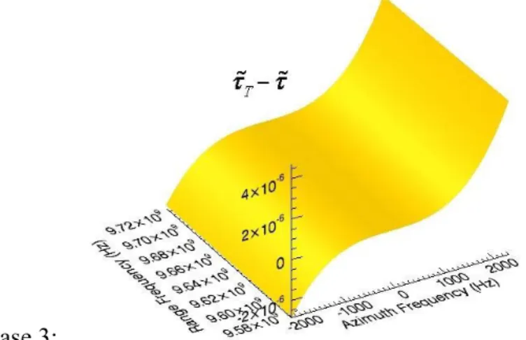
In Figure 14, the difference between the individual PSPs of the transmitter and receiver are plotted against range and azimuth frequencies, for the three above mentioned cases, using the parameters of Table 1.
Case 2:
Case 3:
Figure 14: Difference between the Individual PSPs of the Transmitter and the Receiver In Figure 14, comparing case 1 with cases 2 and 3, we conclude that the difference be-tween the individual PSPs of the transmitter and receiver is considerably decreased by using weighted azimuth contributions of the transmitter and receiver phase terms. Indi-vidual PSPs came closer to each other in case 3 as compared to case 2. Hence, we can say that weighting factor obtained by minimizing square difference between individual PSPs of the transmitter and receiver is optimum as compared to TBP.
2.6.2 Difference between Common and Individual Point of Stationary Phase of the Transmitter
Another approach is to minimize the difference between common and individual PSP of the transmitter. We get the weighting factor by minimizing the square difference between common and the transmitter’s PSP and is given as:


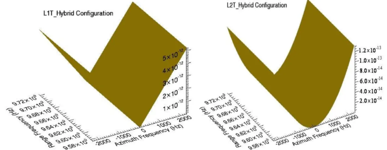

![Figure 35: Focusing Results of Bistatic Azimuth Invariant Configurations: [Left] Opti- Opti-cal Image (Google Maps), [Right] Bistatic SAR Image using a SIFT](https://thumb-us.123doks.com/thumbv2/123dok_us/1309023.2675118/83.892.177.758.309.673/figure-focusing-results-bistatic-azimuth-invariant-configurations-bistatic.webp)

