MPRA
Munich Personal RePEc Archive
Estimation of the Semiparametric Factor
Model: Application to Modelling Time
Series of Electricity Spot Prices.
Dominik Liebl
University of Cologne
2010
Online at
http://mpra.ub.uni-muenchen.de/26800/
Estimation of the Semiparametric Factor Model:
Application to Modelling Time Series of
Electricity Spot Prices.
Dominik Liebl ** Address:
Seminar für Wirtschafts und Sozialstatistik, Lehrstuhl Prof. Mosler, Universität zu Köln, AlbertusMagnusPlatz, 50923 Köln Germany
1 Introduction
Classical univariate and multivariate time series models have problems to deal with the high variability of hourly electricity spot prices. We propose to model alternatively the daily mean electricity supply functions using a dynamic factor model. And to derive, subsequently, the hourly electricity spot prices by the evaluation of the estimated supply functions at the corresponding hourly values of demand for electricity. Supply functions are price (EUR/MWh) functions, that increase monotonically with demand for electric-ity (MW). Apart from this new conceptual approach, that allows us to represent the auction design of energy exchanges in a most natural way, our main contribution is an extraordinary simple algorithm to estimate the factor structure of the dynamic factor model. We decompose the time series into a functional spherical component and an univariate scaling component. The elements of the spherical component are all stan-dardized having unit size such that we can robustly estimate the factor structure. This algorithm is much simpler than procedures suggested in the literature. In order to use a parsimonious labeling we will refer to the daily mean supply curves simply as price curves.
The Dynamic Semiparametric Factor Model (DSFM) of [4] and the follow up applica-tion to electricity spot prices in [3] are close to our approach, but there are two important dierences. Firstly, the authors model the hourly spot prices directly as a multivariate time series and therein fail to mirror the auction design (i.e. the data generating pro-cess) at electricity exchanges. As a result, they are able to explain only about 80% of the variation in hourly spot prices at the European Electricity Exchange while we are able to explain over 98% of the variation using the same number of factors. Secondly, they use an iterating optimization algorithm to estimate the factor structure, whereas we use principal component analysis for sparse functional data [6] to estimate the factor
structure of the spherical component. And we show that the estimated factor structure of the spherical component is also the factor structure of the original series.
2 Functional Dynamic Factor Model
We model the prices, Yti, as observations of an underlying smooth price curve,Xt, such
that
Yti = Xt(uti) +εti witht= 1,2, . . . , T. (1)
Where Xt(.) is a smooth monotone random function of adjusted demand1 u∈ U with
U being a closed and bounded subspace of R. We will set, without loss of generality,
U = [0,1]. The indexi= 1, . . . , Ntinutirefers to thei-th order statistic of the observed
hourly adjusted demand values,uth. The noise term,εti, is assumed to be independently
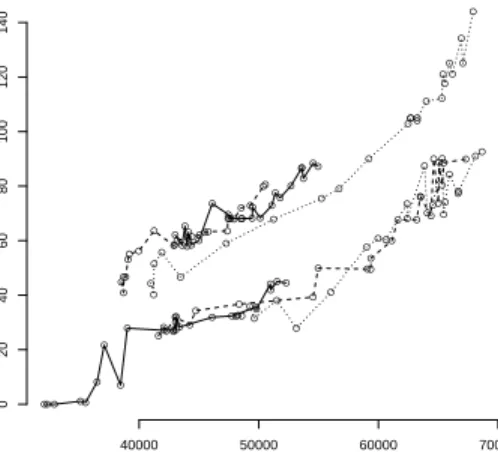
distributed for eachtandi, with E(εti) = 0and Var(εti) =σ2ε. An example of some raw
data vectors Yt = (Yt1, . . . , YtNt)
0 can be seen in gure 1. Note that, some prices Y
ti
have to be treated as outliers, and we useNt to refer to the amount of prices per dayt,
that is used in the estimation procedure. An example of outlier prices can be seen in the left panel of gure 3.
●●● ●● ● ● ● ● ● ●●●● ● ● ● ● ●● ● ●● ● Adjusted Demand (MW) EUR/MWh ●●● ● ● ● ● ● ● ●● ● ● ● ● ● ● ● ● ● ● ● ● ● ●●●●● ● ● ● ●● ● ● ● ● ●● ● ● ● ● ● ● ●● 40000 50000 60000 70000 0 20 40 60 80 100 120 140 ● ● ● ● ● ●● ● ●● ●● ● ● ● ● ● ● ● ● ● ● ●● ● ● ●● ●● ● ● ● ●● ●●●●● ● ●●● ● ● ●● ● ● ● ● ● ● ● ● ● ● ●●●●● ●● ● ● ● ● ● ● ●
Figure 1: Three consecutive days from two dierent arbitrary weeks.
Dynamic factor models are a very successful approach to analyze high dimensional time series data. Our case is a special case of the generalized dynamic factor models
con-sidered in [2] and corresponds to the dynamic factor model in [4]. The factor structure,F,
consists of unknown non parametric functions,f1, . . . , fK, that have to be estimated from
1Adjusted demand means: Original demand values minus electricity from wind-power. Because of its
the data. The K <∞ functionals of the estimated factor structure, Fˆ = [ ˆf1, . . . ,fˆK],
are required to be mutually orthonormal to each other and to be an optimal empirical basis such that
Xt≈ K X k=1 ˆ βtkfˆk = ˆβt0F .ˆ (2)
More precisely, the factor structure, Fˆ = [ ˆf1, . . . ,fˆK], shall dene the best possible
projection from the space HT ⊂L2(U)spanned by the sampled functions, X1, . . . , XT,
into aK dimensional subspace of HT, where best possible is understood with respect
to the mean squared error sense,
T X t=1 ||Xt− K X k=1 ˆ βtkfˆk||22=vmin 1,...,vK T X t=1 min ϑ1,...,ϑK ||Xt− K X k=1 vtkϑk||22, (3)
with respect to all possible ϑ1, . . . , ϑt ∈ L2(U) and vt1, . . . , vtK ∈ R. We use ||.||2
to denote the L2-norm, in its functional version ||f||2 =
q
R1
0 f(u)2du for functions
f ∈L2(U), and its euclidean version ||y||
2 =
q
PN
i=1y 2
i for vectors y ∈RN. Note that
this denition of a factor structure, Fˆ, is also fullled by any rigid rotations, Fˆ∗=TFˆ,
whereTis any orthonormalK×K-matrix such thatTT0 =T0T=I
K.
It is well known that the rstK <∞empirical eigenfunctions, let's sayf1T, . . . , fKT,
of the sample covariance operator,
ρTg = Z 1 0 σT(u, v)g(v)dv, for all g∈L2(U), where σT(u, v) = T−1 T X t=1 Xt(u)Xt(v), with u, v∈ U,
can dene such a best possible projection from the space HT = span(X1, . . . , XT) ⊂
L2(U)into aK-dimensional subspace ofHT. In our general setting, where(X1, . . . , XT)
is allowed to be any collection of functional random variables the sample covariance
op-erator, ρTg, generally does not converge to a population counterpart and the empirical
eigenfunctions and eigenvalues cannot be interpreted as variance components in the
clas-sical sense. This sample dependence of FT = [f1T, . . . , fKT] is not dierent from other
dynamic factor models as in [4].
Unfortunately, given the unrestrictive assumptions on the series (Xt), the spectral
decomposition of the empirical covariance operator, ρTg, generally cannot be used to
estimate a factor structure,FT. As long as the process(Xt)is not stationary, its elements
are likely to be of very dierent orders of magnitude, which will have a dramatic distortion
eect on the sample covariance function, σT. But, contrary to the claim of the authors
in [4], we do not need stationarity in order to use spectral decomposition of the sample
Proposition 2.1 Given the model in (2), if a factor structureFˆ denes the best
projec-tion from the spaceHT =span(X1, . . . , XT) into aK dimensional subspaceHKT ⊂ HT,
then it also denes the best projection from the spaceH∗
T =span( X1
||X1||2, . . . ,
XT
||XT||2)into
the sameK dimensional subspaceHK
T.
This proposition is trivially true, becauseHT =span(X1, . . . , XT)is a vector space and
therefore is closed under scalar multiplication, such that HT = H∗T. Dierent scales
Xtct, with ct 6= 0, will simply cause reciprocal scales of β/cˆ t in the minimization (3).
As a consequence from proposition 2.1 we can also estimate a factor structure for the
original series,(Xt), from the standardized series(||XXt
t||2).
3 The Algorithm
The idea is to decompose the time series,(Yt), into its spherical component that can
be used to estimate the K-dimensional factor structure F and its scaling component
that can be used to rescale the approximated spherical process to its original size. Denition The spherical component of the factor model in equation (2) is given by the multivariate series, Y t−µT(ut) ||Yt−µT(ut)||2 t=1,...,T . (4) Withut= (ut1, . . . , uNt1)andµT =T −1PT
t=1Xtbeing the sample mean function.
Denition The scaling component is given by the univariate series,
(||Yt−µT(ut)||2)t=1,...,T. (5) From a mathematical perspective, it is not necessary to subtract the sample mean,
µT ∈ HT =span(X1, . . . , XT), from the discretization vectors, YT. This simply
sub-tracts the constant vectorβ¯ˆ= (T−1PT
t βˆt1, . . . , T
−1PT
t βˆtK)
0 from the process( ˆβ
t) =
( ˆβt1, . . .βˆtK)0. But, from a practical perspective, the subtraction of the sample mean,
µT, helps to avoid rounding errors caused by oating point computation. Particularly,
when the sizes of dierent vectorsYtare of very dierent orders of magnitude, as in our
application.
By construction, the elements of the spherical component, Yt−µT(ut)
||Yt−µT(ut)||2
, are all of
the same order of magnitude, such that the factor structure,F, can be estimated by the
spectral decomposition of the spherical sample covariance operator, ˜ ρTg = Z 1 0 ˜ σT(u, v)g(v)dv, for all g∈L2(U), where σ˜T(u, v) = T−1 T X t=1 Yt(u)−µT(u) ||Yt(u)−µT(u)||2 Yt(v)−µT(v) ||Yt(v)−µT(v)||2 ,
without distortion eects. This estimation algorithm is by far less costly with respect to computation time and much simpler to implement than the iterative procedure in [4].
4 Application
The estimation of a factor structure,F, for the daily mean electricity supply functions,
Xt, is made a bit more dicult by the sparseness of the data. The observed discretization
points,Yt, of the price functions,Xt, are not uniformly distributed over the whole domain
U = [0,1], but over sub parts of U. This is a slightly dierent form of sparseness as it
is discussed in [5] and [6], where sparseness is referred to the situation with only a few discretization points per function. Nevertheless the smoothing approaches suggested by [5], to estimate the mean function and the covariance operator, as well as the PACE estimation procedure of [6], to estimate the loadings parameters, are directly applicable
to our situation of sparse data. The empirical covariance function,˜σT, and the rst four
factors, f1T, . . . , f4T, can be seen in gure 2. The estimated factor structure explains
about98.5%of the total variance of the price curves, such that we can reduce the high
dimensional problem to aK= 3-dimensional problem without much loss of generality.
r 0.0 0.2 0.4 0.6 0.8 1.0 l 0.0 0.2 0.4 0.6 0.8 1.0 0.01 0.02 0.03 0.04 0.05 0.0 0.2 0.4 0.6 0.8 1.0 0 50 100 150 VARIMX Eigenfun. 1 70.88 % Adjusted Demand (MW) EUR/MWh 0.0 0.2 0.4 0.6 0.8 1.0 0 50 100 150 VARIMX Eigenfun. 2 22.16 % Adjusted Demand (MW) EUR/MWh 0.0 0.2 0.4 0.6 0.8 1.0 0 50 100 150 VARIMX Eigenfun. 3 5.49 % Adjusted Demand (MW) EUR/MWh 0.0 0.2 0.4 0.6 0.8 1.0 0 50 100 150 VARIMX Eigenfun. 4 0.3 % Adjusted Demand (MW) EUR/MWh
Figure 2: Left Panel Empirical covariance function, σ˜T, of the spherical component.
Right Panel First four functionals of the estimated factor structure.
In the left panel of gure 3 we plot one estimated price function,Xˆ
t, of an arbitrary
day,t, with its corresponding raw data vector,Yt, as well as two outlier prices, that are
excluded from the estimation procedure. In the right panel of gure 3 we show hourly electricity spot prices of one arbitrary week. The hourly tted prices are determined by
the evaluation of the estimated price functions,Xˆt, at the corresponding hourly values of
adjusted demand,uth, for electricity. Note, that the proposed dynamic factor model may
be easily combined with already developed approaches to model and forecast demand for electricity such as in [1].
0.0 0.2 0.4 0.6 0.8 1.0 50 100 150 200 250 300 MW EUR/MWh ● ● ●● ● ● ● ● ● ● ● ● ● ● ● ● ● ● ● ● ● ● Hours EUR/MWh 40 60 80 100 120 0 5 10 15 20 25 ● ●●●●● ● ● ●●● ●●●● ●●● ● ● ●● ● Mo. ● ●●●●● ● ●●● ●●●●●●●● ● ● ●●● ● Tu. 0 5 10 15 20 25 ●●●●●●● ● ●● ●● ●●● ●● ● ● ● ● ●●● We. ●●●●●● ● ●●● ●●●●●● ● ● ● ● ● ●● ● Th. ●●●●●● ● ● ●●● ●●●● ●● ● ● ● ● ●● ● Fr. 40 60 80 100 120 ● ● ●●●●●● ● ●● ●● ● ●●● ● ● ● ●●● ● Sa. 40 60 80 100 120 ● ●●●● ●●●● ●● ●● ● ●●● ● ●● ●●●● Su. Orig. Prices Fitted Prices ●
Figure 3: Left Panel Single tted price curve with observed raw prices (circle points) and outlier prices (triangle points). Right Panel Hourly tted prices and original prices.
References
[1] J Antoch, L Prchal, MR Rosa, and P Sarda. Functional linear regression with func-tional response: Application to prediction of electricity consumption. Funcfunc-tional and Operatorial Statistics, pages 52195219, 2008.
[2] M Forni, M Hallin, M Lippi, and M Reichlin. The generalized dynamic factor model: Identication and estimation. The Review of Economics and Statistics, (82): 540554, 2000.
[3] W K Härdle and S Trück. The dynamics of hourly electricity prices. 2010.
[4] B U Park, E Mammen, W Härdle, and S Borak. Time Series Modelling With Semiparametric Factor Dynamics. Journal of the American Statistical Association, 104(485): 284298, 2009.
[5] J G Staniswalis and J J Lee. Nonparametric Regression Analysis of Longitudinal Data. Journal of the American Statistical Association, 93(444): 14031418, 1998. [6] F Yao, H G Müller, and J L Wang. Functional Data Analysis for Sparse Longitudinal