Measuring Generalization and Overfitting in Machine Learning

(1)

UC Berkeley Electronic Theses and Dissertations

Permalink https://escholarship.org/uc/item/6j01x9mz Author Roelofs, Rebecca Publication Date 2019 Peer reviewed|Thesis/dissertation

eScholarship.org Powered by the California Digital Library

(2)

by

Rebecca Roelofs

A dissertation submitted in partial satisfaction of the requirements for the degree of

Doctor of Philosophy in Computer Science in the Graduate Division of the

University of California, Berkeley

Committee in charge:

Professor Benjamin Recht, Co-chair Professor James Demmel, Co-chair

Associate Professor Moritz Hardt Professor Bruno Olshausen

(3)

(4)

Abstract

Measuring Generalization and Overfitting in Machine Learning by

Rebecca Roelofs

Doctor of Philosophy in Computer Science University of California, Berkeley Professor Benjamin Recht, Co-chair Professor James Demmel, Co-chair

Due to the prevalence of machine learning algorithms and the potential for their decisions to profoundly impact billions of human lives, it is crucial that they are robust, reliable, and understandable. This thesis examines key theoretical pillars of machine learning surrounding generalization and overfitting, and tests the extent to which empirical behavior matches existing theory. We develop novel methods for measuring overfitting and generalization, and we characterize how reproducible observed behavior is across differences in optimization algorithm, dataset, task, evaluation metric, and domain.

First, we examine how optimization algorithms bias machine learning models towards solutions with varying generalization properties. We show that adaptive gradient methods empirically find solutions with inferior generalization behavior compared to those found by stochastic gradient descent. We then construct an example using a simple overparameterized model that corroborates the algorithms’ empirical behavior on neural networks.

Next, we study the extent to which machine learning models have overfit to commonly reused datasets in both academic benchmarks and machine learning competitions. We build new test sets for the CIFAR-10 and ImageNet datasets and evaluate a broad range of clas-sification models on the new datasets. All models experience a drop in accuracy, which indicates that current accuracy numbers are susceptible to even minute natural variations in the data distribution. Surprisingly, despite several years of adaptively selecting the models to perform well on these competitive benchmarks, we find no evidence of overfitting. We then analyze data from the machine learning platform Kaggle and find little evidence of substantial overfitting in ML competitions. These findings speak to the robustness of the holdout method across different data domains, loss functions, model classes, and human analysts.

Overall, our work suggests that the true concern for robust machine learning is distribu-tion shift rather than overfitting, and designing models that still work reliably in dynamic environments is a challenging but necessary undertaking.

(5)

(6)

List of Figures

2.1 Training and test errors of various optimization algorithms on CIFAR-10. . . 15 2.2 Performance curves on the training data and the development/test data for three

natural language tasks. . . 18 3.1 Model accuracy on the original CIFAR-10 and ImageNet test sets vs. our new

test sets. . . 22 3.2 Model accuracy on the original ImageNet validation set vs. accuracy on two

vari-ants of our new test set. We refer the reader to Section 3.4 for a description of these test sets. Each data point corresponds to one model in our testbed (shown with 95% Clopper-Pearson confidence intervals). On Threshold0.7, the model ac-curacies are 3% lower than on the original test set. On TopImages, which contains the images most frequently selected by MTurk workers, the models perform 2%

better than on the original test set. The accuracies on both datasets closely fol-low a linear function, similar to MatchedFrequency in Figure 3.1. The red shaded region is a 95% confidence region for the linear fit from 100,000 bootstrap samples. 32 3.3 Randomly selected images from the original and new CIFAR-10 test sets. . . 36 3.4 The pipeline for creating the new ImageNet test set. . . 44 3.5 The user interface employed in the original ImageNet collection process for the

labeling tasks on Amazon Mechanical Turk. . . 47 3.6 Our user interface for labeling tasks on Amazon Mechanical Turk. . . 48 3.7 The user interface we built to review dataset revisions and remove incorrect or

near duplicate images. . . 55 3.8 Probit versus linear scaling for model accuracy comparisons. . . 56 3.9 Impact of the reviewing passes on the accuracy of a resnet152 on our new

MatchedFrequency test set. . . 57 3.10 Model accuracy on the original ImageNet validation set vs. accuracy on the first

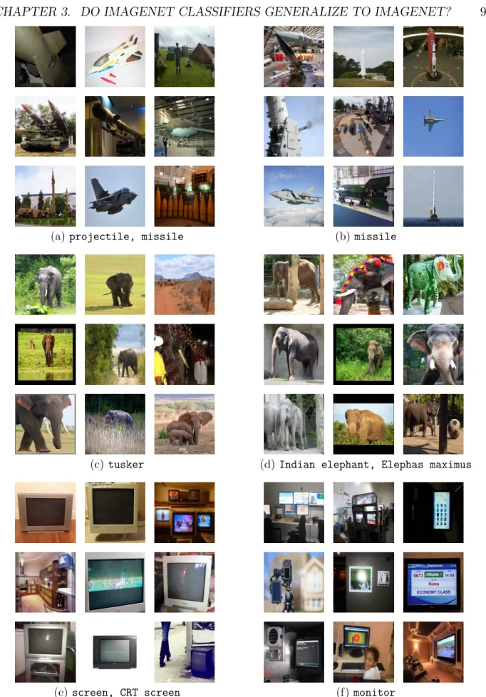
revision of our MatchedFrequency test set. . . 58 3.11 Hard images from our new test set that no model correctly. The caption of

each image states the correct class label (“True”) and the label predicted by most models (“Predicted”). . . 70 3.12 Model accuracy on the original ImageNet validation set vs. each of our new test

(10)

3.13 Model accuracy on the original ImageNet validation set vs. our new test sets using probit scale. . . 92 3.14 Randomly selected images from the original ImageNet validation set and our new

ImageNet test sets. . . 93 3.15 Model accuracy on the new test set stratified by selection frequency bin. . . 94 3.16 Model accuracy on the original test set stratified by selection frequency bin. . . 95 3.17 Stratified model accuracies on the original ImageNet validation set versus

accu-racy on our new test set MatchedFrequency . . . 96 3.18 Random images from the original ImageNet validation set for three pairs of classes with

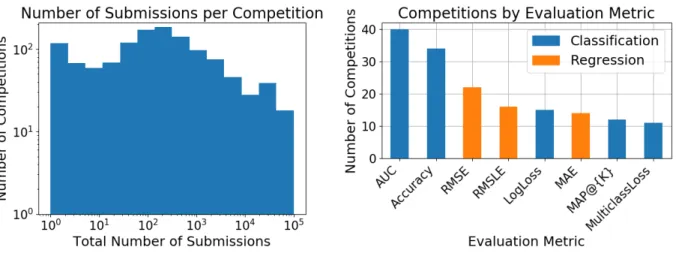
ambiguous class boundaries. . . 97 4.1 Overview of the Kaggle competitions. The left plot shows the distribution of

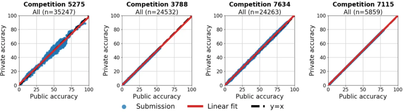
submissions per competition. The right plot shows the score types that are most common among the competitions with at least 1,000 submissions. . . 101 4.2 Private versus public accuracy for all submissions for the most popular Kaggle

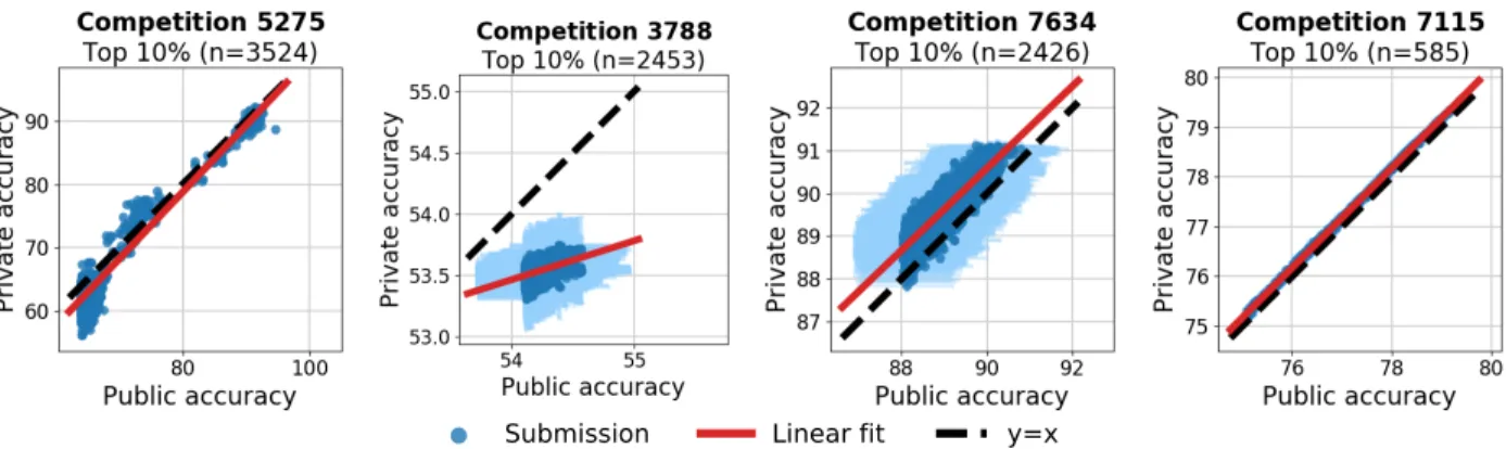
accuracy competitions. . . 104 4.3 Private versus public accuracy for the top 10% of submissions for the most popular

Kaggle accuracy competitions. . . 105 4.4 Empirical CDFs of the p-values for three (sub)sets of submissions in the four

accuracy competitions with the largest number of submissions. . . 106 4.5 Empirical CDF of the mean accuracy differences for Kaggle accuracy competitions

and mean accuracy difference vs. competition end date. . . 108 4.6 Empirical CDF of mean score differences for 40 AUC competitions, 12 MAP@K

competitions, 15 LogLoss competitions, and 11 MulticlassLoss competitions. . . 110 4.7 Mean accuracy difference outlier competitions . . . 115 4.8 Private versus public accuracy for all submissions for the most popular Kaggle

accuracy competitions. . . 117 4.8 Private versus public accuracy for all submissions for the most popular Kaggle

accuracy competitions. . . 118 4.9 Private versus public accuracy for top 10% of submissions for the most popular

Kaggle accuracy competitions. . . 120 4.9 Private versus public accuracy for all submissions for the most popular Kaggle

accuracy competitions. . . 121 4.10 Competitions whose empirical CDFs agree with the idealized null model that

assumes no overfitting . . . 122 4.11 Empirical CDFs for an idealized null model that assumes no overfitting for all

Kaggle accuracy competitions. . . 123 4.11 Empirical CDFs for an idealized null model that assumes no overfitting for all

Kaggle accuracy competitions. . . 124 4.12 Private versus public AUC for all submissions for Kaggle AUC competitions. . 130 4.12 Private versus public AUC for all submissions for Kaggle AUC competitions. . . 131

(11)

4.13 Private versus public accuracy for top 10% of submissions for Kaggle AUC com-petitions. . . 133 4.13 Private versus public AUC for top 10% of submissions for Kaggle AUC competitions.134 4.14 Private versus public MAP@K for all submissions for Kaggle MAP@K competitions.136 4.15 Private versus public MAP@K for top 10% of submissions for Kaggle MAP@K

competitions. . . 137 4.16 Private versus public MulticlassLoss for all submissions for Kaggle MulticlassLoss

competitions. . . 140 4.17 Private versus public MulticlassLoss for top 10% of submissions for Kaggle

Mul-ticlassLoss competitions. . . 141 4.18 Private versus public LogLoss for all submissions for Kaggle LogLoss competitions.143 4.19 Private versus public LogLoss for top 10% of submissions for Kaggle LogLoss

competitions. . . 144 4.20 Mean score differences versus competition end date for all classification evaluation

(12)

List of Tables

2.1 Parameter settings of optimization algorithms used in deep learning. . . 8 2.2 Summary of the model architectures, datasets, and frameworks used in deep

learning experiments. . . 13 2.3 Default hyperparameters for algorithms in deep learning frameworks. . . 19 3.1 Model accuracies on the original CIFAR-10 test set, the original ImageNet

vali-dation set, and our new test set. . . 27 3.2 Impact of the three sampling strategies for our ImageNet test sets. . . 31 3.3 Human accuracy on the “hardest” images in the original and our new CIFAR-10

test set. . . 39 3.4 Model accuracies on cross-validation splits for the original CIFAR-10 data. . . . 40 3.5 Accuracies for discriminator models trained to distinguish between the original

and new CIFAR-10 test sets. . . 41 3.6 resnet50 accuracy on cross-validation splits created from the original ImageNet

train and validation sets. . . 53 3.7 Distribution of the top 25 keywords in each class for the new and original test set. 64 3.12 Model accuracy on the original CIFAR-10 test set and our new test set. . . 71 3.13 Model accuracy on the original CIFAR-10 test set and the exactly class-balanced

variant of our new test set. . . 72 3.14 Top-1 model accuracy on the original ImageNet validation set and our new test

set MatchedFrequency. . . 77 3.15 Top-5 model accuracy on the original ImageNet validation set and our new test

set MatchedFrequency. . . 79 3.16 Top-1 model accuracy on the original ImageNet validation set and our new test

set Threshold0.7. . . 81 3.17 Top-5 model accuracy on the original ImageNet validation set and our new test

set Threshold0.7. . . 83 3.18 Top-1 model accuracy on the original ImageNet validation set and our new test

set TopImages. . . 85 3.19 Top-5 model accuracy on the original ImageNet validation set and our new test

(13)

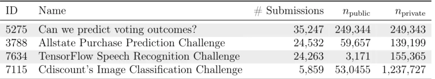
4.1 The four Kaggle accuracy competitions with the largest number of submissions. 103

4.2 Competitions scored with accuracy with greater than 1000 submissions. . . 113

4.3 Competitions scored with AUC with greater than 1000 submissions. . . 126

4.3 Competitions scored with AUC with greater than 1000 submissions. . . 127

4.4 Competitions scored with MAP@K with greater than 1000 submissions. . . 135

4.5 Competitions scored with MulticlassLoss with greater than 1000 submissions. . . 138

(14)

Acknowledgments

First, thank you to my advisors Benjamin Recht and James Demmel. I am lucky to have studied under such intelligent, hard working, and creative scientists. Ben and I arrived at Berkeley at the same time, and his first topics class, The Mathematics of Information and Data, exposed me to interesting and challenging problems at the intersection of statistical machine learning and optimization, and eventually inspired me to change the course of my Ph.D. work. I also credit my interest and knowledge in parallel computing and numerical linear algebra to Jim’s research agenda and courses.

Thank you to Shivaram Venkatarman for mentoring me during my early years of gradu-ate school. Shivaram taught me the fundamentals of empirical research in machine learning, and his knowledge of systems and programming was indispensable. One of the most memo-rable bugs that we found together involved discovering that DORMQR was not thread-safe. Shivaram is now both a role model and a friend, and I truly admire his kindness, patience, and willingness to answer any question.

Thank you to my collaborators Sara Fridovich-Keil, Moritz Hardt, John Miller, Mitchell Stern, Ludwig Schmidt, Vaishaal Shankar, and Nathan Srebro, Stephen Tu, and Ashia Wil-son. Without all of their hard work, this thesis would not be possible.

My experience at Berkeley was shaped by the people I was surrounded by. Overall, I found Berkeley to be a fun, collaborative environment, and it was a joy to go to work with some of the most brilliant and kind people I knew. Special thanks to Orianna DeMassi, Esther Rolf, Evan Sparks, Eric Jonas, Nikolai Matni, Ross Boczar, Stephen Tu, Horia Mania, Max Simchowitz, Sarah Dean, Lydia Liu, Karl Krauth, Wenshuo Guo, Vickie Ye, Ben Brock, Marquita Ellis, Michael Driscoll, Penporn Koanatakool, and William Kahan.

Lastly, thank you to my family who inspired me to pursue a Ph.D. and showed me that science could be an enjoyable and fruitful career. Yoyo especially deserves my utmost gratitude for listening to me rehearse talks over and over again, helping me navigate difficult professional situations, and editing drafts of this thesis. Above all, I am appreciative of the love and support I received from my family. This thesis is dedicated to them.

(15)

Chapter 1 Introduction

Over the past decade, an increasingly broad and diverse set of industries have deployed machine learning as a key component of their services. Technological innovations that trans-formed streams of data into fire hydrants, as well as ubiquitous economic pressures for automation, fueled the growing adoption of machine learning. Today, law enforcement, employment decisions, admissions, credit scoring, social networks, search results, and ad-vertising all commonly use machine learning algorithms. Once deployed, these algorithms quickly achieve massive reach, and their decisions can potentially affect the lives of billions of people. In some application areas, such as medical diagnoses and self-driving cars, decisions made by machine learning algorithms can also have serious repercussions for human safety. Since machine learning algorithms now have the power to shape and influence all aspects of society at unprecedented scale, it is critical that the algorithms are robust, reliable, and understandable. However, as we push the technology into more challenging application areas, weaknesses have emerged.

One shortcoming is that current classifiers are extremely sensitive to small shifts in the underlying data distribution. This fragility to distribution shift hinders the ability of the algorithm to generalize, or handle unseen or novel situations. For example, a self-driving car trained to drive on city streets would have difficulty driving on highways. Ultimately, the algorithm’s lack of generalization causes it to make incorrect decisions, some of which have severe consequences. Moreover, distributional sensitivity leaves the underlying algorithms vulnerable to attack from malicious adversaries; by changing the underlying data in a way that is imperceptible to humans, an adversary can easily manipulate specific predictions made by the algorithm.

A related weakness of machine learning algorithms is that they are notoriously difficult to interpret. When mistakes inevitably occur, it is challenging to identify what aspect of the data or system caused the mistake and how one should fix the problem. Even among machine learning experts, there is a lack of understanding for how or why a machine learning system arrives at a certain decision, in part because much of the success of machine learning has been driven by empirical progress, with little guidance from theory. The majority of published papers have embraced a paradigm where the main justification for a new learning technique

(16)

is its improved performance on a few key benchmarks, yet there are few explanations as to

why a proposed technique achieves a reliable improvement over prior work.

Deep neural networks, in particular, have proved difficult to analyze from a theoretical perspective. Several architectural components and optimization techniques—for example, batch normalization, residual connections, extreme overfitting, and increasing step sizes— work exceedingly well in practice but have little theoretical justification. While there has been some progress in analyzing these phenomena [82, 17, 18], our current theoretical under-standing is not rich enough to predict practical behavior. As a result, our ability to propose novel innovations that improve existing networks is limited.

The goal of this thesis is to empirically examine key theoretical pillars of machine learning so that we can build algorithms that are more reliable and robust. If we can understand and identify precisely where the breakdowns between theory and practice occur, we can create a body of knowledge that is reproducible across many settings, giving us the tools we need to both recognize the limitations of existing algorithms and improve their ability to adapt to novel situations.

At a high level, the analysis we perform exhibits a common pattern: In each case, we isolate a key phenomenon, either originating from existing theory or “conventional wisdom”, and then rigorously test the range of settings under which the phenomenon holds. We focus on how the phenomenon changes as we individually vary core parts of the machine learning system, such as the optimization algorithm, the data, the hypothesis class, and the task objective. We then verify how well the behavior we observe empirically matches existing theory.

One theme that arises in the thesis is that measurement matters. We cannot build our theoretical understanding of the principles that govern robustness and reliability without accurate measurements of generalization. One issue that arises immediately from the theo-retical definition of generalization error is that the exact quantity of interest is impossible to evaluate because it requires knowing the underlying population distribution. We can use approximations to bypass this difficulty, but it is important to know what assumptions we use when we make these approximations and to be aware of situations where we break these assumptions. As we rely more and more on machine learning for real-world, safety-critical applications, our models must be robust to small shifts in the underlying data distribution. To achieve robustness, we must be able to measure it.

1.1 Formal background on generalization and overfitting

“Generalization” and “overfitting” are widely used throughout machine learning as umbrella terms; generalization is often interpreted as the broad ability of a classifier to handle new scenarios while overfitting is used to describe any unwanted performance drop of a machine learning model. In this section, we provide formal background that allows us to define more precisely the notions of generalization and overfitting that we use throughout the rest of the thesis.

(17)

1.1.1 Generalization error

In statistical learning theory, our goal is to predict an outcome y from a set Y of possible outcomes, given that we observe x from some feature space X. Our input is a dataset of n

labeled examples

S ={(x1, y1), . . . ,(xn, yn)} (1.1.1) which we use to choose a function f :X → Y so that given a new pair(x, y), f(x)is a good approximation to y. The classic approach to measuring how wellf(x) predictsy is to define a loss function l : Y × Y → _R which intuitively represents the cost of predicting yˆ= f(x) when the true label is y.

We adopt the standard probabilistic assumption and posit the existence of a “true” underlying data distribution D over labeled examples (x, y). We assume that the pairs (x1, y1), . . . ,(xn, yn) in our sample are chosen independently and identically from the data distributionD. Then, we wish to choose f so that we minimize the expected population risk

LD(f) =E[l(f(x), y)] (1.1.2)

where the expectation is taken with respect to the draw of (x, y) fromD.

However, since we often do not know the exact form of the data distributionD, we cannot always evaluate the expectation needed to compute the population risk. Instead, we use our sample S to evaluate the empirical loss

LS(f) = 1 n n X i=1 l(f(xi), yi). (1.1.3)

We then minimize the empirical loss to learn a function fˆn such that

ˆ

fn= arg min f

LS(f) (1.1.4)

We use the subscript n on fˆn to denote explicitly that f depends on the sample S =

{(x1, y1), . . . ,(xn, yn)}. Here, S is the training set, the empirical loss is akin to the training loss, and the process of finding the function fˆn that minimizes the empirical loss is the process of training a model.

The generalization error G of fˆn is the difference between the empirical loss and the population loss

G=LD( ˆfn)−LS( ˆfn). (1.1.5) Since we do not know how to evaluate LD, we rely on another sample Stest∼ D to estimate

the population loss. Then, we compute an approximate generalization error Gˆ as ˆ

G=LStest( ˆfn)−LS( ˆfn). (1.1.6)

In deep learning, a trained model often achieves a training loss of 0 (i.e. LS( ˆfn) = 0), so we also sometimes assume that

ˆ

(18)

In Chapter 2 we use the trained model’s performance on the test set as a proxy for the model’s generalization error. However, as we discuss next and revisit in Chapters 3 and 4, this approximation critically assumes that we have not used the test set to select the trained model.

1.1.2 Adaptive overfitting

In this thesis, we focus on adaptive overfitting, which is overfitting caused by test set reuse. When defining generalization error, we assumed that the model learned from the training set

ˆ

fn does not depend on the test set Stest. This assumption underlies essentially all empirical

evaluations in machine learning since it allows us to argue that the modelfˆngeneralizes. As long as the modelfˆndoes not depend on the test setStest, standard concentration results [83]

show thatLStest( ˆfn)is a good approximation of the true performance given by the population

lossLD( ˆfn).

However, machine learning practitioners often undermine this assumption by selecting models and tuning hyperparameters based on the test loss. Especially when algorithm designers evaluate a large number of different models on the same test set, the final classifier may only perform well on the specific examples in the test set. The failure to generalize to the entire data distribution D manifests itself in a large adaptivity gap LD( ˆfn)−LStest( ˆfn)

and leads to overly optimistic performance estimates.

In practice, ifStesthas been used to selectfˆn, we must draw a new test setStest0 ∼ Dthat

is independent of fˆn to evaluate the empirical loss as an approximation to the population loss LD( ˆfn). Then, we can empirically measure the amount of adaptive overfitting as the difference between the empirical loss on the new test set and the empirical loss on the original test set

LS0

test( ˆfn)−LStest( ˆfn) (1.1.8)

In Chapters 3 and 4 we exploit this strategy to explore to what extent adaptive overfitting occurs in popular machine learning benchmarks and competitions.

1.2 Dissertation overview

The goal of the thesis is to ensure that machine learning algorithms are robust and reliable. Our approach is to empirically evaluate key theoretical pillars of machine learning in order to better understand robustness. We explore how changing key components of a machine learning system, such as the dataset, the architecture, the task type, the evaluation metric, or the optimization algorithm, impact empirical measurements of generalization and overfitting. First, Chapter 2 explores the impact of the optimization algorithm on generalization error. We demonstrate that adaptive gradient methods can find solutions that have worse generalization error when compared to the more traditional stochastic gradient descent.

Next, Chapter 3 explores the impact of the dataset on generalization error and adaptive overfitting. We create new test sets for CIFAR-10 and ImageNet that allow us to measure the

(19)

amount of adaptive overfitting on these popular benchmarks. Surprisingly, we find little to no evidence of adaptive overfitting despite the fact that these benchmarks have been reused intensively for almost a decade for model selection.

Finally, Chapter 4 explores the impact of both the task and evaluation metric when measuring adaptive overfitting in machine learning competitions. We conduct the first large meta-analysis of overfitting due to test set reuse in the machine learning community, ana-lyzing over one hundred machine learning competitions on the Kaggle platform. Our longi-tudinal study shows, somewhat surprisingly, little evidence of substantial overfitting

(20)

Chapter 2 Generalization properties of adaptive

gradient methods

Adaptive optimization methods, which perform local optimization with a metric constructed from the history of iterates, are becoming increasingly popular for training deep neural networks. Examples include AdaGrad, RMSProp, and Adam. In this chapter, we discuss the generalization properties of adaptive gradient methods and compare these to the more traditional stochastic gradient descent (SGD).

2.1 Introduction

An increasing share of deep learning researchers are training their models with adaptive gradient methods [19, 64] due to their rapid training time [46]. Adam [50] in particular has become the default algorithm used across many deep learning frameworks. However, the generalization and out-of-sample behavior of such adaptive gradient methods remains poorly understood. Given that many passes over the data are needed to minimize the training objective, typical regret guarantees do not necessarily ensure that the found solutions will generalize [77].

Notably, when the number of parameters exceeds the number of data points, it is possible that the choice of algorithm can dramatically influence which model is learned [69]. Given two different minimizers of some optimization problem, what can we say about their relative ability to generalize? In this paper, we show that adaptive and non-adaptive optimization methods indeed find very different solutions with very different generalization properties. We provide a simple generative model for binary classification where the population is linearly separable (i.e., there exists a solution with large margin), but AdaGrad [19], RMSProp [91], and Adam converge to a solution that incorrectly classifies new data with probability arbi-trarily close to half. On this same example, SGD finds a solution with zero error on new data. Our construction shows that adaptive methods tend to give undue influence to spurious features that have no effect on out-of-sample generalization (defined as in 1.1.7).

(21)

We additionally present numerical experiments demonstrating that adaptive methods generalize less well than their non-adaptive counterparts. Our experiments reveal three primary findings. First, with the same amount of hyperparameter tuning, SGD and SGD with momentum outperform adaptive methods on the test set across all evaluated models and tasks. This is true even when the adaptive methods achieve the same training loss or lower than non-adaptive methods. Second, adaptive methods often display faster initial progress on the training set, but their performance quickly plateaus on the test set. Third, the same amount of tuning was required for all methods, including adaptive methods. This challenges the conventional wisdom that adaptive methods require less tuning. Moreover, as a useful guide to future practice, we propose a simple scheme for tuning learning rates and decays that performs well on all deep learning tasks we studied.

2.2 Background

The canonical optimization algorithms used to minimize risk are either stochastic gradient methods or stochastic momentum methods. Stochastic gradient methods can generally be written

wk+1 =wk−αk∇˜f(wk), (2.2.1)

where ∇˜f(wk) :=∇f(wk;xik) is the gradient of some loss function f computed on a batch

of data xik.

Stochastic momentum methods are a second family of techniques that have been used to accelerate training. These methods can generally be written as

wk+1 =wk−αk∇˜f(wk+γk(wk−wk−1)) +βk(wk−wk−1). (2.2.2) The sequence of iterates (2.2.2) includes Polyak’s heavy-ball method (HB) with γk = 0, and Nesterov’s Accelerated Gradient method (NAG) [85] with γk =βk.

Notable exceptions to the general formulations (2.2.1) and (2.2.2) are adaptive gradient and adaptive momentum methods, which choose a local distance measure constructed us-ing the entire sequence of iterates (w1,· · · , wk). These methods (including AdaGrad [19], RMSProp [91], and Adam [50]) can generally be written as

wk+1 =wk−αkH−k1∇˜f(wk+γk(wk−wk−1)) +βkH−k1Hk−1(wk−wk−1), (2.2.3) where Hk :=H(w1,· · · , wk)is a positive definite matrix. Though not necessary, the matrix

Hk is usually defined as Hk = diag   ( _k X i=1 ηigi◦gi )1/2 , (2.2.4)

where “◦” denotes the entry-wise or Hadamard product,gk= ˜∇f(wk+γk(wk−wk−1)), andηk is some set of coefficients specified for each algorithm. That is,Hkis a diagonal matrix whose

(22)

entries are the square roots of a linear combination of squares of past gradient components. We will use the fact thatHkare defined in this fashion in the sequel. For the specific settings of the parameters for many of the algorithms used in deep learning, see Table 2.1. Adaptive methods attempt to adjust an algorithm to the geometry of the data. In contrast, stochastic gradient descent and related variants use the `2 geometry inherent to the parameter space, and are equivalent to setting Hk = I in the adaptive methods.

SGD HB NAG AdaGrad RMSProp Adam

Gk I I I Gk−1+ Dk β2Gk−1+ (1−β2)Dk ₁₋β2_βk 2 Gk−1+ (1 −β2) 1−βk 2 Dk αk α α α α α α₁1−₋β_β1k 1 βk 0 β β 0 0 β1(1−βk₁−1) 1−βk 1 γ 0 0 β 0 0 0

Table 2.1: Parameter settings of optimization algorithms used in deep learning. Here,Dk=

diag(gk◦gk) and Gk := Hk◦Hk. We omit the additional added to the adaptive methods, which is only needed to ensure non-singularity of the matrices Hk.

In this context,generalization refers to the performance of a solutionwon a broader pop-ulation. Performance is often defined in terms of a different loss function than the function

f used in training. For example, in classification tasks, we typically define generalization in terms of classification error rather than cross-entropy.

2.2.1 Related work

Understanding how optimization relates to generalization is a very active area of current machine learning research. Most of the seminal work in this area has focused on understand-ing how early stoppunderstand-ing can act as implicit regularization [100]. In a similar vein, Ma and Belkin [60] have shown that gradient methods may not be able to find complex solutions at all in any reasonable amount of time. Hardt et al. [77] show that SGD is uniformly stable, and therefore solutions with low training error found quickly will generalize well. Similarly, using a stability argument, Raginsky et al. [74] have shown that Langevin dynamics can find solutions that generalize better than ordinary SGD in non-convex settings. Neyshabur, Srebro, and Tomioka [69] discuss how algorithmic choices can act as implicit regularizer. In a similar vein, Neyshabur, Salakhutdinov, and Srebro [68] show that a different algorithm, one which performs descent using a metric that is invariant to re-scaling of the parameters, can lead to solutions which sometimes generalize better than SGD. Our work supports the work of [68] by drawing connections between the metric used to perform local optimization and the ability of the training algorithm to find solutions that generalize. However, we focus primarily on the different generalization properties of adaptive and non-adaptive methods.

A similar line of inquiry has been pursued by Keskar et al. [49]. Horchreiter and Schmid-huber [36] showed that “sharp” minimizers generalize poorly, whereas “flat” minimizers

(23)

gen-eralize well. Keskar et al. empirically show that Adam converges to sharper minimizers when the batch size is increased. However, they observe that even with small batches, Adam does not find solutions whose performance matches state-of-the-art. In the current work, we aim to show that the choice of Adam as an optimizer itself strongly influences the set of minimiz-ers that any batch size will ever see, and help explain why they were unable to find solutions that generalized particularly well.

2.3 The perils of preconditioning

The goal of this section is to illustrate the following observation: when a problem has multiple global minima, different algorithms can find entirely different solutions. In particular, we will show that adaptive gradient methods might find very poor solutions. To simplify the presentation, let us restrict our attention to the simple binary least-squares classification problem, where we can easily compute closed form formulae for the solutions found by different methods. In least-squares classification, we aim to solve

minimizew RS[w] :=kXw−yk22. (2.3.1) HereX is an n×d matrix of features andy is an n-dimensional vector of labels in {−1,1}. We aim to find the best linear classifier w. Note that when d > n, if there is a minimizer with loss 0 then there is an infinite number of global minimizers. The question remains: what solution does an algorithm find and how well does it generalize to unseen data?

2.3.1 Non-adaptive methods

Most common methods when applied to (2.3.1) will find the same solution. Indeed, any gradient or stochastic gradient of RS must lie in the span of the rows of X. Therefore, any method that is initialized in the row span of X (say, for instance at w = 0) and uses only linear combinations of gradients, stochastic gradients, and previous iterates must also lie in the row span ofX. The unique solution that lies in the row span ofXalso happens to be the solution with minimum Euclidean norm. We thus denotewSGD₌_XT₍_XXT₎−1_y_{. Almost all} non-adaptive methods like SGD, SGD with momentum, mini-batch SGD, gradient descent, Nesterov’s method, and the conjugate gradient method will converge to this minimum norm solution. Minimum norm solutions have the largestmargin, or distance between the decision boundary and the closest data point to the decisioun boundary, out of all solutions of the equation Xw =y. Maximizing margin has a long and fruitful history in machine learning, and thus it is a pleasant surprise that gradient descent naturally finds a max-margin solution.

2.3.2 Adaptive methods

Let us now consider the case of adaptive methods, restricting our attention to diagonal adap-tation. While it is difficult to derive the general form of the solution, we can analyze special

(24)

cases. Indeed, we can construct a variety of instances where adaptive methods converge to solutions with low `∞ norm rather than low `2 norm.

For a vector x∈ _Rq_{, let} _sign(_x₎ _{denote the function that maps each component of} _x _to its sign.

Lemma 2.3.1. SupposeXTy has no components equal to0 and there exists a scalar csuch that X sign(XT_y_{) =} _cy_{. Then, when initialized at} _w

0 = 0, AdaGrad, Adam, and RMSProp

all converge to the unique solution w∝sign(XT_y₎_.

In other words, whenever there exists a solution of Xw = y that is proportional to sign(XT_y₎_{, this is precisely the solution to where all of the adaptive gradient methods} con-verge.

Proof. We prove this lemma by showing that the entire trajectory of the algorithm consists of iterates whose components have constant magnitude. In particular, we will show that

wk =λk sign(XTy).

for some scalar λk. Note that w0 = 0 satisfies the assertion with λ0 = 0. Now, assume the assertion holds for all k≤t. Observe that

∇RS(wk+γk(wk−wk−1)) =XT(X(wk+γk(wk−wk−1))−y)

=XT (λk+γk(λk−λk−1))X sign(XTy)−y

={(λk+γk(λk−λk−1))c−1}XTy

=µkXTy,

where the last equation defines µk. Hence, letting gk =∇RS(wk+γk(wk−wk−1)), we also have Hk = diag   ( _k X s=1 ηs gs◦gs )1/2 = diag   ( _k X s=1 ηsµ2s )1/2 |XTy|  =νkdiag |XTy|

where|u|denotes the component-wise absolute value of a vector and the last equation defines

νk. Thus we have, wk+1 =wk−αkH−k1∇f(wk+γk(wk−wk−1)) +βtH−k1Hk−1(wk−wk−1) (2.3.2) = λk− αkµk νk + βkνk−1 νk (λk−λk−1) sign(XTy) (2.3.3)

proving the claim.

Note that this solution wcould be obtained without any optimization at all. One simply could subtract the means of the positive and negative classes and take the sign of the resulting vector. This solution is far simpler than the one obtained by gradient methods, and it would be surprising if such a simple solution would perform particularly well. We now turn to showing that such solutions can indeed generalize arbitrarily poorly.

(25)

2.3.3 Adaptivity can overfit

Lemma 2.3.1 allows us to construct a particularly pernicious generative model where Ada-Grad fails to find a solution that generalizes. This example uses infinite dimensions to simplify bookkeeping, but one could take the dimensionality to be 6n. Note that in deep learning, we often have a number of parameters equal to 25n or more [90], so this is not a particularly high dimensional example by contemporary standards. For i= 1, . . . , n, sample the label yi to be 1 with probability pand −1with probability 1−pfor some p >1/2. Let

x be an infinite dimensional vector with entries

xij =          yi j = 1 1 j = 2,3 1 j = 4 + 5(i−1), . . . ,4 + 5(i−1) + 2(1−yi) 0 otherwise .

In other words, the first feature of xi is the class label. The next 2 features are always equal to 1. After this, there is a set of features unique to xi that are equal to 1. If the class label is 1, then there is 1 such unique feature. If the class label is −1, then there are 5 such features. Note that for such a data set, the only discriminative feature is the first one! Indeed, one can perform perfect classification using only the first feature. The other features are all useless. Features 2 and 3 are constant, and each of the remaining features only appear for one example in the data set. However, as we will see, algorithms without such a priori knowledge may not be able to learn these distinctions.

Take n samples and consider the AdaGrad solution to the minimizing||Xw−y||2_{. First} we show that the conditions of Lemma 2.3.1 hold. Let b=Pn

i=1yi and assume for the sake of simplicity that b >0. This will happen with arbitrarily high probability for large enough

n. Define u=XTy and observe that

uj =      n j = 1 b j = 2,3 yj if j >3 and xj = 1 and sign(uj) =      1 j = 1 1 j = 2,3 yj if j >3 and xj = 1 Thus we have hu, xii =yi+ 2 +yi(3−2yi) = 4yi, as desired. Hence, the AdaGrad solution

wada _∝ _sign(_u₎_{. In particular,} _wada _{has all of its components either equal to} ₀ _{or to} _±_τ _for some positive constant τ. Now since wada _{has the same sign pattern as} _u_{, the first three} components ofwadaare equal to each other. But for a new data point,xtest, the only features that are nonzero in both xtest _and _wada _{are the first three. In particular, we have}

hwada, xtesti=τ(y(test)+ 2)>0.

Therefore, the AdaGrad solution will label all unseen data as being in the positive class! Now let’s turn to the minimum norm solution. Let P and N denote the set of positive and negative examples respectively. Let n+ = |P| and n− = |N |. By symmetry, we have

(26)

that the minimum norm solution will have the form wSGD = P

i∈P α+xi −P_j∈N α−xj for some nonnegative scalarsα+ and α−. These scalars can be found by solving XXTα=y. In

closed form we have

α+= 4n−+ 3 9n++ 3n−+ 8n+n−+ 3 and α−= 4n++ 1 9n++ 3n−+ 8n+n−+ 3 . (2.3.4) The algebra required to compute these coefficients can be found in Section 2.3.4. For a new data point,xtest, again the only features that are nonzero in both xtestandwSGD are the first three. Thus we have

hwSGD, xtesti=ytest(n+α++n−α−) + 2(n+α+−n−α−).

Using (2.3.4), we see that whenevern+> n−/3, the SGD solution makes no errors.

Though this generative model was chosen to illustrate extreme behavior, it shares salient features of many common machine learning instances. There are a few frequent features, where some predictor based on them is a good predictor, though these might not be easy to identify from first inspection. Additionally, there are many other features which are very sparse. On finite training data it looks like such features are good for prediction, since each such feature is very discriminatory for a particular training example, but this is over-fitting and an artifact of having fewer training examples then features. Moreover, we will see shortly that adaptive methods typically generalize worse than their non-adaptive counterparts on real datasets as well.

2.3.4 Why SGD converges to the minimum norm solution

The simplest derivation of the minimum norm solution uses the kernel trick. We know that the optimal solution has the form wSGD=XTαwhere α=K−1yand K =XXT. Note that

Kij =          4 if i=j and yi = 1 8 if i=j and yi =−1 3 if i6=j and yiyj = 1 1 if i6=j and yiyj =−1

Positing that αi =α+ if yi = 1 and α+i=α− if yi =−1 leaves us with the equation

(3n++ 1)α+−n−α− = 1 −n+α++ (3n−+ 3)α− = 1

(27)

Name Network type Architecture Dataset Framework

C1 Deep Convolutional cifar.torch CIFAR-10 Torch

L1 2-Layer LSTM torch-rnn War & Peace Torch

L2 2-Layer LSTM + Feedforward span-parser Penn Treebank DyNet

L3 3-Layer LSTM emnlp2016 Penn Treebank Tensorflow

Table 2.2: Summary of the model architectures, datasets, and frameworks used in deep learning experiments. 1

2.4 Deep learning experiments

Having established that adaptive and non-adaptive methods can find quite different solutions in the convex setting, we now turn to an empirical study of deep neural networks to see whether we observe a similar discrepancy in generalization. We compare two non-adaptive methods – SGD and the heavy ball method (HB) – to three popular adaptive methods – AdaGrad, RMSProp and Adam. We study performance on four deep learning problems:

(C1) the CIFAR-10 image classification task, (L1) character-level language modeling on the novel War and Peace, and (L2) discriminative parsing and (L3) generative parsing on Penn Treebank. In the interest of reproducibility, we use a network architecture for each problem that is either easily found online (C1, L1, L2, and L3) or produces state-of-the-art results (L2 and L3). Table 2.2 summarizes the setup for each application. We take care to make minimal changes to the architectures and their data pre-processing pipelines in order to best isolate the effect of each optimization algorithm.

We conduct each experiment 5 times from randomly initialized starting points, using the initialization scheme specified in each code repository. We allocate a pre-specified budget on the number of epochs used for training each model. When a development set was available, we chose the settings that achieved the best peak performance on the development set by the end of the fixed epoch budget. CIFAR-10 did not have an explicit development set, so we chose the settings that achieved the lowest training loss at the end of the fixed epoch budget.

Our experiments show the following primary findings: (i) Adaptive methods find solu-tions that generalize worse than those found by non-adaptive methods. (ii) Even when the adaptive methods achieve the same training loss or lower than non-adaptive methods, the development or test performance is worse. (iii) Adaptive methods often display faster initial progress on the training set, but their performance quickly plateaus on the development set. (iv) Though conventional wisdom suggests that Adam does not require tuning, we find that tuning the initial learning rate and decay scheme for Adam yields significant improvements over its default settings in all cases.

1_{Architectures can be found at the following links: (1)}_cifar.torch_: _{https://github.com/szagoruyk}

o/cifar.torch; (2) torch-rnn: https://github.com/jcjohnson/torch-rnn; (3) span-parser: https: //github.com/jhcross/span-parser; (4)emnlp2016: https://github.com/cdg720/emnlp2016.

(28)

2.4.1 Hyperparameter tuning

Optimization hyperparameters have a large influence on the quality of solutions found by optimization algorithms for deep neural networks. The algorithms under consideration have many hyperparameters: the initial step size α0, the step decay scheme, the momentum value β0, the momentum schedule βk, the smoothing term , the initialization scheme for the gradient accumulator, and the parameter controlling how to combine gradient outer products, to name a few. A grid search on a large space of hyperparameters is infeasible even with substantial industrial resources, and we found that the parameters that impacted performance the most were the initial step size and the step decay scheme. We left the remaining parameters with their default settings. We describe the differences between the default settings of Torch, DyNet, and Tensorflow in Section 2.6.1 for completeness.

To tune the step sizes, we evaluated a logarithmically-spaced grid of five step sizes. If the best performance was ever at one of the extremes of the grid, we would try new grid points so that the best performance was contained in the middle of the parameters. For example, if we initially tried step sizes 2, 1, 0.5, 0.25, and 0.125 and found that 2 was the best performing, we would have tried the step size 4 to see if performance was improved. If performance improved, we would have tried 8 and so on. We list the initial step sizes we tried in Section 2.6.2.

For step size decay, we explored two separate schemes, a development-based decay scheme (dev-decay) and a fixed frequency decay scheme (fixed-decay). For dev-decay, we keep track of the best validation performance so far, and at each epoch decay the learning rate by a constant factorδif the model does not attain a new best value. For fixed-decay, we decay the learning rate by a constant factor δ every k epochs. We recommend the dev-decay scheme when a development set is available; not only does it have fewer hyperparameters than the fixed frequency scheme, but our experiments also show that it produces results comparable to, or better than, the fixed-decay scheme.

2.4.2 Convolutional neural network

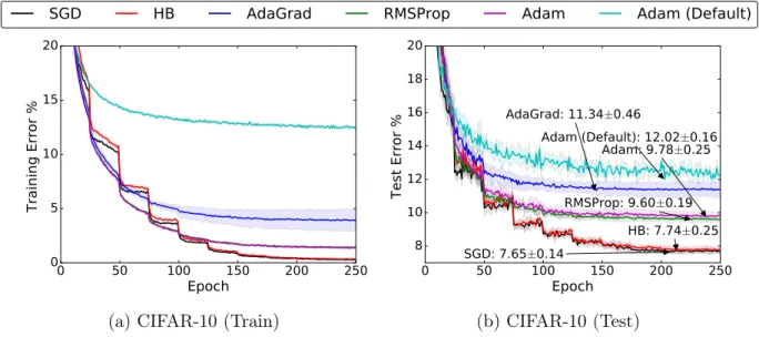
We used the VGG+BN+Dropout network for CIFAR-10 from the Torch blog [101], which in prior work achieves a baseline test error of 7.55%. Figure 2.1 shows the learning curve for each algorithm on both the training and test dataset.

We observe that the solutions found by SGD and HB do indeed generalize better than those found by adaptive methods. The best overall test error found by a non-adaptive algorithm, SGD, was 7.65±0.14%, whereas the best adaptive method, RMSProp, achieved a test error of 9.60±0.19%.

Early on in training, the adaptive methods appear to be performing better than the non-adaptive methods, but starting at epoch 50, even though the training error of the non-adaptive methods is still lower, SGD and HB begin to outperform adaptive methods on the test error. By epoch 100, the performance of SGD and HB surpass all adaptive methods on both train and test. Among all adaptive methods, AdaGrad’s rate of improvement flatlines the

(29)

0 50 100 150 200 250

Epoch

0 5 10 15 20

Training Error %

(a) CIFAR-10 (Train)

0 50 100 150 200 250

Epoch

8 10 12 14 16 18 20

Test Error %

SGD: 7.65±0.14 HB: 7.74±0.25 AdaGrad: 11.34±0.46 RMSProp: 9.60±0.19 Adam: 9.78±0.25 Adam (Default): 12.02±0.16 (b) CIFAR-10 (Test)

Figure 2.1: Training (left) and top-1 test error (right) on CIFAR-10. The annotations indicate where the best performance is attained for each method. The shading represents

± one standard deviation computed across five runs from random initial starting points. In all cases, adaptive methods are performing worse on both train and test than non-adaptive methods.

earliest. We also found that by increasing the step size, we could drive the performance of the adaptive methods down in the first 50 or so epochs, but the aggressive step size made the flatlining behavior worse, and no step decay scheme could fix the behavior.

2.4.3 Character-Level language modeling

Using the torch-rnn library, we train a character-level language model on the text of the novel War and Peace, running for a fixed budget of 200 epochs. Our results are shown in Figures 2.2a and 2.2b.

Under the fixed-decay scheme, the best configuration for all algorithms except AdaGrad was to decay relatively late with regards to the total number of epochs, either 60 or 80% through the total number of epochs and by a large amount, dividing the step size by 10. The dev-decay scheme paralleled (within the same standard deviation) the results of the exhaustive search over the decay frequency and amount; we report the curves from the fixed policy.

Overall, SGD achieved the lowest test loss at 1.212±0.001. AdaGrad has fast initial progress, but flatlines. The adaptive methods appear more sensitive to the initialization scheme than non-adaptive methods, displaying a higher variance on both train and test. Surprisingly, RMSProp closely trails SGD on test loss, confirming that it is not impossible for adaptive methods to find solutions that generalize well. We note that there are step

(30)

configurations for RMSProp that drive the training loss below that of SGD, but these con-figurations cause erratic behavior on test, driving the test error of RMSProp above Adam.

2.4.4 Constituency parsing

A constituency parser is used to predict the hierarchical structure of a sentence, breaking it down into nested clause-level, phrase-level, and word-level units. We carry out experi-ments using two state-of-the-art parsers: the stand-alone discriminative parser of Cross and Huang [12], and the generative reranking parser of Choe and Charniak [7]. In both cases, we use the dev-decay scheme with δ= 0.9for learning rate decay.

Discriminative model. Cross and Huang [12] develop a transition-based framework that reduces constituency parsing to a sequence prediction problem, giving a one-to-one corre-spondence between parse trees and sequences of structural and labeling actions. Using their code with the default settings, we trained for 50 epochs on the Penn Treebank [63], compar-ing labeled F1 scores on the traincompar-ing and development data over time. RMSProp was not implemented in the used version of DyNet, and we omit it from our experiments. Results are shown in Figures 2.2c and 2.2d.

We find that SGD obtained the best overall performance on the development set, followed closely by HB and Adam, with AdaGrad trailing far behind. The default configuration of Adam without learning rate decay actually achieved the best overall training performance by the end of the run, but was notably worse than tuned Adam on the development set.

Interestingly, Adam achieved its best development F1 of 91.11 quite early, after just 6 epochs, whereas SGD took 18 epochs to reach this value and didn’t reach its best F1 of 91.24 until epoch 31. On the other hand, Adam continued to improve on the training set well after its best development performance was obtained, while the peaks for SGD were more closely aligned.

Generative model. Choe and Charniak [7] show that constituency parsing can be cast as a language modeling problem, with trees being represented by their depth-first traver-sals. This formulation requires a separate base system to produce candidate parse trees, which are then rescored by the generative model. Using an adapted version of their code base,2 _{we retrained their model for 100 epochs on the Penn Treebank. However, to reduce}

computational costs, we made two minor changes: (a) we used a smaller LSTM hidden di-mension of 500 instead of 1500, finding that performance decreased only slightly; and (b) we accordingly lowered the dropout ratio from 0.7 to 0.5. Since they demonstrated a high correlation between perplexity (the exponential of the average loss) and labeled F1 on the 2_{While the code of Choe and Charniak treats the entire corpus as a single long example, relying on the} network to reset itself upon encountering an end-of-sentence token, we use the more conventional approach of resetting the network for each example. This reduces training efficiency slightly when batches contain examples of different lengths, but removes a potential confounding factor from our experiments.

(31)

development set, we explored the relation between training and development perplexity to avoid any conflation with the performance of a base parser.

Our results are shown in Figures 2.2e and 2.2f. On development set performance, SGD and HB obtained the best perplexities, with SGD slightly ahead. Despite having one of the best performance curves on the training dataset, Adam achieves the worst development perplexities.

2.5 Conclusion

Despite the fact that our experimental evidence demonstrates that adaptive methods are not advantageous for machine learning, the Adam algorithm remains incredibly popular. We are not sure exactly as to why, but hope that our step-size tuning suggestions make it easier for practitioners to use standard stochastic gradient methods in their research. In our conversations with other researchers, we have surmised that adaptive gradient methods are particularly popular for training GANs [79, 43] and Q-learning with function approxima-tion [66, 56]. Both of these applicaapproxima-tions stand out because they are not solving optimizaapproxima-tion problems. It is possible that the dynamics of Adam are accidentally well matched to these sorts of optimization-free iterative search procedures. It is also possible that carefully tuned stochastic gradient methods may work as well or better in both of these applications. It is an exciting direction of future work to determine which of these possibilities is true and to understand better as to why.

(32)

0 50 100 150 200

Epoch

1.04 1.06 1.08 1.10 1.12 1.14 1.16 1.18 1.20

Training Loss

(a) War and Peace (Training Set)

0 50 100 150 200

Epoch

1.20 1.22 1.24 1.26 1.28 1.30 1.32 1.34

Test Loss

SGD: 1.212±0.001 HB: 1.218±0.002 AdaGrad: 1.233±0.004 RMSProp: 1.214±0.005 Adam: 1.229±0.004 Adam (Default): 1.269±0.007

(b) War and Peace (Test Set)

10 20 30 40 50

Epoch

86 88 90 92 94 96 98

Training F1

(c) Discriminative Parsing (Training Set)

10 20 30 40 50

Epoch

89.0 89.5 90.0 90.5 91.0 91.5 92.0

Development F1

AdaGrad: 90.18±0.03 Adam (Default): 90.79±0.13 Adam: 91.11±0.09 HB: 91.16±0.12 SGD: 91.24±0.11

(d) Discriminative Parsing (Development Set) 20 40 60 80 100

Epoch

4.4 4.6 4.8 5.0 5.2 5.4 5.6 5.8 6.0

Training Perplexity

(e) Generative Parsing (Training Set)

20 40 60 80 100

Epoch

5.0 5.2 5.4 5.6 5.8 6.0

Development Perplexity

SGD: 5.09±0.04 HB: 5.13±0.01 AdaGrad: 5.24±0.02 RMSProp: 5.28±0.00 Adam: 5.35±0.01 Adam (Default): 5.47±0.02

(f) Generative Parsing (Development Set)

Figure 2.2: Performance curves on the training data (left) and the development/test data (right) for three experiments on natural language tasks. The annotations indicate where the best performance is attained for each method. The shading represents one standard deviation computed across five runs from random initial starting points.

(33)

2.6 Supplementary material

2.6.1 Differences between Torch, DyNet, and Tensorflow

Torch Tensorflow DyNet

SGD Momentum 0 No default 0.9

AdaGrad Initial Mean 0 0.1 0

AdaGrad 1e-10 Not used 1e-20

RMSProp Initial Mean 0 1.0 –

RMSProp β 0.99 0.9 –

RMSProp 1e-8 1e-10 –

Adam β1 0.9 0.9 0.9

Adam β2 0.999 0.999 0.999

Table 2.3: Default hyperparameters for algorithms in deep learning frameworks. Table 2.3 lists the default values of the parameters for the various deep learning packages used in our experiments. In Torch, the Heavy Ball algorithm is callable simply by changing default momentum away from 0 withnesterov=False. In Tensorflow and DyNet, SGD with momentum is implemented separately from ordinary SGD. For our Heavy Ball experiments we use a constant momentum of β = 0.9.

2.6.2 Step sizes used for parameter tuning

CIFAR-10

• SGD: {2, 1, 0.5 (best), 0.25, 0.05, 0.01}

• HB: {2, 1, 0.5 (best), 0.25, 0.05, 0.01}

• AdaGrad: {0.1, 0.05, 0.01 (best, def.), 0.0075, 0.005}

• RMSProp: {0.005, 0.001, 0.0005, 0.0003 (best), 0.0001}

• Adam: {0.005, 0.001 (default), 0.0005, 0.0003 (best), 0.0001, 0.00005}

The default Torch step sizes for SGD (0.001) , HB (0.001), and RMSProp (0.01) were outside the range we tested.

War & Peace

• SGD: {2, 1 (best), 0.5, 0.25, 0.125}

(34)

• AdaGrad: {0.4, 0.2, 0.1, 0.05 (best), 0.025}

• RMSProp: {0.02, 0.01, 0.005, 0.0025, 0.00125, 0.000625, 0.0005 (best), 0.0001}

• Adam: {0.005, 0.0025, 0.00125, 0.000625 (best), 0.0003125, 0.00015625}

Under the fixed-decay scheme, we selected learning rate decay frequencies from the set

{10,20,40,80,120,160,∞}and learning rate decay amounts from the set{0.1,0.5,0.8,0.9}. Discriminative Parsing

• SGD: {1.0, 0.5, 0.2, 0.1 (best), 0.05, 0.02, 0.01}

• HB: {1.0, 0.5, 0.2, 0.1, 0.05 (best), 0.02, 0.01, 0.005, 0.002}

• AdaGrad: {1.0, 0.5, 0.2, 0.1, 0.05, 0.02 (best), 0.01, 0.005, 0.002, 0.001, 0.0005, 0.0002, 0.0001}

• RMSProp: Not implemented in DyNet.

• Adam: {0.01, 0.005, 0.002 (best), 0.001 (default), 0.0005, 0.0002, 0.0001} Generative Parsing

• SGD: {1.0, 0.5 (best), 0.25, 0.1, 0.05, 0.025, 0.01}

• HB: {0.25, 0.1, 0.05, 0.02, 0.01 (best), 0.005, 0.002, 0.001}

• AdaGrad: {5.0, 2.5, 1.0, 0.5, 0.25 (best), 0.1, 0.05, 0.02, 0.01}

• RMSProp: {0.05, 0.02, 0.01, 0.005, 0.002 (best), 0.001, 0.0005, 0.0002, 0.0001}

(35)

Chapter 3 Do ImageNet classifiers generalize to

ImageNet?

3.1 Introduction

The overarching goal of machine learning is to produce models that generalize. We usually quantify generalization by measuring the performance of a model on a held-out test set. What does good performance on the test set then imply? At the very least, one would hope that the model also performs well on a new test set assembled from the same data source by following the same data cleaning protocol.

In this chapter, we realize this thought experiment by replicating the dataset creation process for two prominent benchmarks, CIFAR-10 and ImageNet [53, 15]. In contrast to the ideal outcome, we find that a wide range of classification models fail to reach their original accuracy scores. The accuracy drops range from 3% to 15% on CIFAR-10 and 11% to 14% on ImageNet. On ImageNet, the accuracy loss amounts to approximately five years of progress in a highly active period of machine learning research.

Conventional wisdom suggests that such drops arise because the models have been adapted to the specific images in the original test sets, e.g., via extensive hyperparameter tuning. However, our experiments show that the relative order of models is almost exactly preserved on our new test sets: the models with highest accuracy on the original test sets are still the models with highest accuracy on the new test sets. Moreover, there are no dimin-ishing returns in accuracy. In fact, every percentage point of accuracy improvement on the original test set translates to a larger improvement on our new test sets. So although later models could have been adapted more to the test set, they see smaller drops in accuracy. These results provide evidence that exhaustive test set evaluations are an effective way to improve image classification models. Adaptivity is therefore an unlikely explanation for the accuracy drops.

Instead, we propose an alternative explanation based on the relative difficulty of the original and new test sets. We demonstrate that it is possible to recover the original ImageNet

(36)

accuracies almost exactly if we only include the easiest images from our candidate pool. This suggests that the accuracy scores of even the best image classifiers are still highly sensitive to minutiae of the data cleaning process. This brittleness puts claims about human-level performance into context [47, 33, 81]. It also shows that current classifiers still do not generalize reliably even in the benign environment of a carefully controlled reproducibility experiment.

Figure 3.1 shows the main result of our experiment. Before we describe our methodology in Section 3.3, the next section provides relevant background. To enable future research, we release both our new test sets and the corresponding code.1

80 90 100

Original test accuracy (%)

70 80 90 100

New test accuracy (%)

CIFAR-10

60 70 80

Original test accuracy (top-1, %)

40 50 60 70 80

New test accuracy (top-1, %)

ImageNet

Ideal reproducibility

Model accuracy

Linear fit

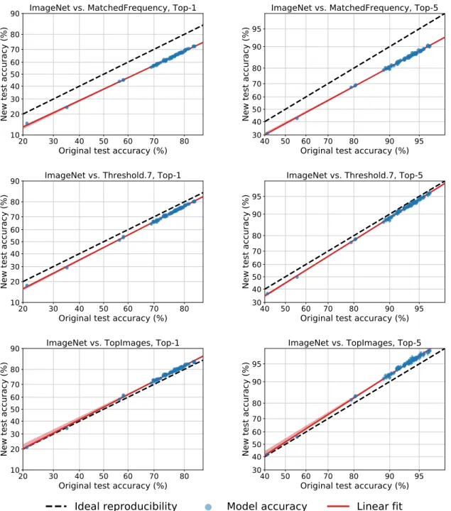
Figure 3.1: Model accuracy on the original test sets vs. our new test sets. Each data point corresponds to one model in our testbed (shown with 95% Clopper-Pearson confidence intervals). The plots reveal two main phenomena: (i) There is a significant drop in accuracy from the original to the new test sets. (ii) The model accuracies closely follow a linear function with slope greater than 1 (1.7 for CIFAR-10 and 1.1 for ImageNet). This means that every percentage point of progress on the original test set translates into more than one percentage point on the new test set. The two plots are drawn so that their aspect ratio is the same, i.e., the slopes of the lines are visually comparable. The red shaded region is a 95% confidence region for the linear fit from 100,000 bootstrap samples.

3.2 Potential causes of accuracy drops

We adopt the standard classification setup and posit the existence of a “true” underlying data distributionD over labeled examples (x, y). The overall goal in classification is to find

1

https://github.com/modestyachts/CIFAR-10.1 and https://github.com/modestyachts/ImageN etV2

(37)

a model fˆthat minimizes the population loss LD( ˆf) = _E (x,y)∼D h I[ ˆf(x)6=y] i . (3.2.1)

Since we usually do not know the distribution D, we instead measure the performance of a trained classifier via a test set Stest drawn from the distributionD:

LStest( ˆf) = 1 |Stest| X (x,y)∈Stest I[ ˆf(x)6=y]. (3.2.2)

We then use this test errorLStest( ˆf)as a proxy for the population loss LD( ˆf). If a model

ˆ

f achieves a low test error, we assume that it will perform similarly well on future examples from the distribution D. This assumption underlies essentially all empirical evaluations in machine learning since it allows us to argue that the model fˆgeneralizes.

In our experiments, we test this assumption by collecting a new test set S_test0 from a data distributionD0 _{that we carefully control to resemble the original distribution}_D_{. Ideally, the}

original test accuracyLStest( ˆf) and new test accuracy LS0_test( ˆf) would then match up to the

random sampling error. In contrast to this idealized view, our results in Figure 3.1 show a large drop in accuracy from the original test set Stest set to our new test set Stest0 . To

understand this accuracy drop in more detail, we decompose the difference betweenLStest( ˆf)

and LS0test( ˆf)into three parts (dropping the dependence on

ˆ

f to simplify notation):

LStest −LStest0 = (LStest−LD)

| {z } Adaptivity gap + (LD−LD0) | {z } Distribution Gap + (LD0−L_S0 test) | {z } Generalization gap .

We now discuss to what extent each of the three terms can lead to accuracy drops.

Generalization gap. By construction, our new test setS_test0 is independent of the existing classifier fˆ. Hence the third term LD0 −L_S0

test is the standardgeneralization gap commonly

studied in machine learning. It is determined solely by the random sampling error.

A first guess is that this inherent sampling error suffices to explain the accuracy drops in Figure 3.1 (e.g., the new test set S_test0 could have sampled certain “harder” modes of the distributionDmore often). However, random fluctuations of this magnitude are unlikely for the size of our test sets. With 10,000 data points (as in our new ImageNet test set), a Clopper-Pearson 95% confidence interval for the test accuracy has size of at most ±1%. Increasing the confidence level to 99.99% yields a confidence interval of size at most ±2%. Moreover, these confidence intervals become smaller for higher accuracies, which is the relevant regime for the best-performing models. Hence random chance alone cannot explain the accuracy drops observed in our experiments.2

2_{We remark that the sampling process for the new test set} _S0

test could indeed systematically sample harder modes more often than under the original data distribution D. Such a systematic change in the sampling process would not be an effect of random chance but captured by the distribution gap described below.

(38)

Adaptivity gap. We call the termLStest−LD the adaptivity gap. It measures how much

adapting the model fˆto the test set Stest causes the test error LStest to underestimate the

population loss LD. If we assumed that our modelfˆis independent of the test setStest, this

terms would follow the same concentration laws as the generalization gapLD0−L_S0

test above.

But this assumption is undermined by the common practice of tuning model hyperparameters directly on the test set, which introduces dependencies between the model fˆand the test set Stest. In the extreme case, this can be seen as training directly on the test set. But

milder forms of adaptivity may also artificially inflate accuracy scores by increasing the gap between LStest and LD beyond the purely random error.

Distribution gap. We call the termLD−LD0 the distribution gap. It quantifies how much

the change from the original distribution D to our new distribution D0 _{affects the model} ˆ

f. Note that this term is not influenced by random effects but quantifies the systematic difference between sampling the original and new test sets. While we went to great lengths to minimize such systematic differences, in practice it is hard to argue whether two high-dimensional distributions are exactly the same. We typically lack a precise definition of either distribution, and collecting a real dataset involves a plethora of design choices.

3.2.1 Distinguishing between the two mechanisms

For a single model fˆ, it is unclear how to disentangle the adaptivity and distribution gaps. To gain a more nuanced understanding, we measure accuracies formultiple modelsfˆ1, . . . ,fˆk. This provides additional insights because it allows us to determine how the two gaps have evolved over time.

For both CIFAR-10 and ImageNet, the classification models come from a long line of papers that incrementally improved accuracy scores over the past decade. A natural as-sumption is that later models have experienced more adaptive overfitting since they are the result of more successive hyperparameter tuning on the same test set. Their higher accu-racy scores would then come from an increasing adaptivity gap and reflect progress only on the specific examples in the test set Stest but not on the actual distribution D. In an

extreme case, the population accuracies LD( ˆfi) would plateau (or even decrease) while the test accuracies LStest( ˆfi) would continue to grow for successive modelsfˆi.

However, this idealized scenario is in stark contrast to our results in Figure 3.1. Later models do not see diminishing returns but anincreased advantage over earlier models. Hence we view our results as evidence that the accuracy drops mainly stem from a large distribution gap. After presenting our results in more detail in the next section, we will further discuss this point in Section 3.7.

Measuring Generalization and Overfitting in Machine Learning

UC Berkeley Electronic Theses and Dissertations

Contents

List of Figures

List of Tables

Acknowledgments

Chapter 1

Introduction

1.1

Formal background on generalization and overfitting

1.1.1

Generalization error

1.1.2

Adaptive overfitting

1.2

Dissertation overview

Chapter 2

Generalization properties of adaptive

gradient methods

2.1

Introduction

2.2

Background

2.2.1

Related work

2.3

The perils of preconditioning

2.3.1

Non-adaptive methods

2.3.2

Adaptive methods

2.3.3

Adaptivity can overfit

2.3.4

Why SGD converges to the minimum norm solution

2.4

Deep learning experiments

2.4.1

Hyperparameter tuning

2.4.2

Convolutional neural network

Epoch

Training Error %

Epoch

Test Error %

2.4.3

Character-Level language modeling

2.4.4

Constituency parsing

2.5

Conclusion

Epoch

Training Loss

Epoch

Test Loss

Epoch

Training F1

Epoch

Development F1

Epoch

Training Perplexity

Epoch

Development Perplexity

2.6

Supplementary material

2.6.1

Differences between Torch, DyNet, and Tensorflow

2.6.2

Step sizes used for parameter tuning

Chapter 3

Do ImageNet classifiers generalize to

ImageNet?

3.1

Introduction

Original test accuracy (%)

New test accuracy (%)

CIFAR-10

Original test accuracy (top-1, %)

New test accuracy (top-1, %)

ImageNet