Learning nonlinear monotone classifiers using the Choquet Integral

LEARNING

NONLINEAR

M

ONOTONE

CLASSIFIERS

USING

THE

CHOQUET

I

NTEGRAL

Dissertation

zur Erlangung des Doktorgrades der Naturwissenschaften

(Dr. rer. nat.)

dem Fachbereich Mathematik und Informatik der Philipps-Universität Marburg

vorgelegt

von

Ali Fallah Tehrani

Vom Fachbereich Mathematik und Informatik der Philipps-Universität Marburg als Dissertation angenommen am: 17.06.2014

Erstgutachter: Prof. Dr. rer. nat. Eyke Hüllermeier Zweitgutachter: Dr. Krzysztof Dembczy´nski Tag der mündlichen Prüfung: 20.06.2014

Contents

1 Introduction 3

1.1 Prior Knowledge . . . 4

1.2 Monotonicity as a Specific Type of Prior Knowledge . . . 4

1.2.1 Medicine . . . 5

1.2.2 Buying a Car . . . 5

1.3 Monotonicity and Multiple Criteria Decision Making . . . 6

1.3.1 The Choquet Integral . . . 6

1.4 The Choquet Integral and its Contribution to Machine Learning 6 2 Background in Machine Learning 9 2.1 Introduction . . . 9 2.2 Supervised Learning . . . 9 2.2.1 Basic Setting . . . 10 2.2.2 Loss Functions . . . 11 2.2.3 Binary Classification . . . 12 2.2.4 Ordinal Classification . . . 13

2.3 The Principles of Induction . . . 13

2.3.1 Maximum Likelihood Estimation (MLE) . . . 13

2.3.2 Structural Risk Minimization (SRM) . . . 15

2.4 The Methods Derived from Inductive Principles . . . 19

2.4.1 Linear Logistic Regression . . . 19

2.4.2 Margin Maximization Principle . . . 21

2.4.3 Kernel Methods . . . 25

2.5 Monotone Classifiers . . . 27

3 The Choquet Integral as an Aggregation Function 29 3.1 Multiple Criteria Decision Making . . . 30

3.1.1 Introduction . . . 30

3.1.3 Aggregation Functions . . . 33

3.2 The Choquet Integral as an Extension of Lebesgue Integral . . 34

3.3 Fuzzy Measures . . . 34

3.3.1 Non-Additive Measures . . . 35

3.3.2 Fuzzy Measures and their Möbius Transforms . . . 35

3.3.3 Monotonicity Constraints . . . 36

3.3.4 k-additivity . . . 37

3.4 The Discrete Choquet Integral . . . 37

3.5 An Application of the Choquet Integral in MCDM . . . 40

3.6 Interpretability of the Choquet Integral . . . 42

3.6.1 Shapley Index . . . 42

3.6.2 Interaction Index . . . 43

4 Monotone Learning by Using the Choquet Integral - Maximum Likelihood Approach 47 4.1 Algorithms for Learning Monotone Binary Classifiers . . . 48

4.1.1 Linear Logistic Regression . . . 48

4.1.2 Choquistic Regression . . . 51

4.1.3 Maximum Likelihood Estimation . . . 53

4.2 Algorithms for Learning Monotone Ordinal Classifiers . . . . 55

4.2.1 Ordinal Logistic Regression . . . 55

4.2.2 Maximum Likelihood Estimation . . . 57

4.2.3 Ordinal Choquistic Regression . . . 61

4.2.4 Maximum Likelihood Estimation . . . 62

4.3 Related Researches . . . 63

5 Kernel-Based Learning and Support Vector Machines 71 5.1 Learning the Choquet Integral by Employing SVM . . . 72

5.1.1 Primal Form . . . 72

5.1.2 Dual Form . . . 74

5.2 The Choquet Kernels . . . 75

6 Capacity Control 81 6.1 Under VC Dimension of the Choquet Integral . . . 83

6.2 Regularization . . . 86

6.2.1 L1-Regularization . . . 86

6.2.2 Hierarchical Regularization . . . 87

6.3 Complexity Reduction . . . 89

6.3.2 2-additive Choquet Integral . . . 92

6.4 Measure Correction - From non Monotone Measure to Mono-tone Measure . . . 96

7 Data Sets and Experimental Parts 109 7.1 Data Description . . . 109

7.2 Normalization . . . 112

7.3 Methods . . . 113

7.4 Experimental Results Regarding Binary Class Classification . 113 7.5 Experimental Results Related to Measure Correction . . . 119

7.6 Experimental Results Regarding Ordinal Class Classification . 122 7.7 Experimental Results for Complexity Reduction . . . 124

7.8 Experimental Results with Respect to Running Time . . . 125

7.8.1 2-additive Choquet Integral . . . 125

7.8.2 The Choquet Kernel . . . 128

7.9 Interpretation and Illustration . . . 129

8 Conclusion & Outlook 135 8.1 Conclusion . . . 135

List of Figures

2.1 The Illustration of VC dimension for Linear Model Class . . . 16

2.2 The Illustration of Structural Risk Minimization . . . 18

2.3 The Illustration of Large Margin Approach . . . 23

2.4 The Illustration of Soft Margin Approach . . . 24

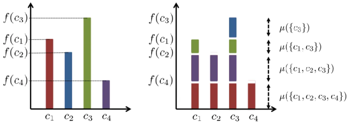
3.1 The Illustration of the Discrete Choquet Integral for4Criteria 39

4.1 The Illustration of Choquistic Regression for Different Values

ofγ . . . 53

4.2 The Illustration of the Ordinal Logistic Regression . . . 57

4.3 The Illustration of the Ordinal Choquistic Regression for 4

Ordinal Classes . . . 61

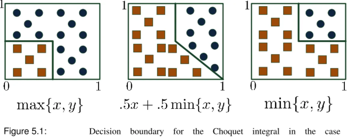
5.1 Visualization of Decision Boundary in the case of Binary

Clas-sification and Different Values for Möbius Transform . . . 74

6.1 Illustrative of Hierarchical Regularization . . . 88

6.2 Illustrative of Directed Acyclic Graph Representing

Mono-tonicity . . . 97

7.1 The Illustration of Average Runtime for SDW Data in2-additive

Choquistic Regression . . . 128

7.2 The Illustration of Run Time with Respect to Primal and Dual

Setting for the Case of the Choquet Kernel . . . 129

7.3 Visualization of the Interaction Index for the Car Evaluation . 131

7.4 Visualization of the Interaction Index for Color Yield in Polyester

Dyeing . . . 132

7.5 Illustrative Scatterplot Visualizations of the Data under

7.6 The Illustration of Satisfying Monotonicity Constraints for Different Datasets . . . 134

List of Tables

7.1 Data sets and their properties . . . 112

7.2 The methods and their abbreviations . . . 113

7.3 Classification performance in terms of the mean and standard

deviation of 0/1 loss . . . 116 7.4 Win statistics (number of data sets on which the first method was

better than the second one) for 20%, 50%, and 80% training data for 0/1 loss case. . . 117

7.5 Classification accuracy for2-additive choquistic regression . . 118

7.6 The comparison of average errors for different kernels respect

to binary classification . . . 120 7.7 Win statistics (number of data sets on which the first method was

better than the second one) for 80% training data for 0/1 loss case. . 121

7.8 The comparison results for two different approaches

under-lying fuzzy measure correction. . . 121

7.9 The comparison results for two different approaches

under-lying fuzzy measure correction. . . 121 7.10 Ordinal classification performance in terms of the mean and

standard deviation ofL1loss . . . 123

7.11 Performance in terms the average Error±standard deviation for dimensionality reduction case (=δ =.1). . . 124 7.12 Runtime complexity of the different methods measured in terms

of CPU time (mean±standard deviation) for different sample sizes (in%of the complete data set). . . 126 7.13 Average values of the scaling parameter γ in the choquistic

Acknowledgment

This thesis would not have been completed, without support and help from a many people. I would like to take this opportunity to appreciate the academics as well my family and my friends.

In this regard, first and foremost I would like to express my sincere appreci-ation to my supervisor, Prof. Dr. Eyke Hüllermeier, who acquainted me with a new field interdisciplinary computer science, statistics and mathematics. During my PhD, Prof. Hüllermeier has oriented me by proposing numerous great ideas and perspectives. His logical way of thinking always improved notably my initial ideas, and specifically his advices enhanced the structure of this dissertation. I am as well deeply grateful. For me, coming from the theoretical informatics and mathematics community, this was an ideal opportunity to discover and to use sound mathematical and statistical tools to solve real challenging problems from an artificial intelligence point of view. I am very thankful to him for giving me the opportunity to explore this area and support me during the PhD.

Also I would like to take this opportunity to thank my collaborators as well my colleagues at Philipps Universität Marburg. From them I learned many useful ideas. In this respect, I would like to thank Dr. Krzysztof Dembczy´nski, Dr. Christophe Labreuche, Dr. Marc Strickert, Dr. Thomas Fober, Dr. Weiwei Cheng, Dr. Robert Busa-Fekete, Maryam Nassiri, Ammar Shaker, Robin Senge, Amira Abdel-Aziz, Florian Meyer, Michael Bräuning, Dr. Willem Waegeman, Sascha Henzgen, Dr. Marco Mernberger, Dirk Schäfer, Manish Agarwal, Dr. Anne Knöller, Patrice Schlegel and Dr. Hyung won Koh.

Especially I appreciate the efforts of Krzysztof, Marc, Thomas and Weiwei.

I owe so much to my family and my friends for supporting me during my edu-cation, specifically my PhD. My special thanks and appreciations go to my parents and my sister, who during this time interval were considerate and always giving

positive energy and encouraging me to my research and my PhD. Nina, I am deeply indebted to you for everything that you done for the family.

Summary

The learning of predictive models that guarantee a monotonic relationship between the output (response) and input (predictor) variables has received increasing atten-tion in machine learning in recent years. While being less problematic for linear models, the difficulty of ensuring monotonicity increases with the flexibility of the underlying model class.

This thesis advocates the so-called Choquet integral as a mathematical tool for learning monotone nonlinear models for classification. While being widely used as a flexible aggregation function in fields such as multiple criteria decision mak-ing, the Choquet integral is much less known in machine learning so far. Apart from combining monotonicity and flexibility in a mathematically sound and elegant manner, the Choquet integral has additional features making it attractive from a ma-chine learning point of view. For example, it offers measures for quantifying the importance of individual predictor variables and the interaction between groups of variables, thereby supporting the interpretability of a model.

Concrete methods for learning with the Choquet integral are developed on the basis of two different approaches, namely maximum likelihood estimation and struc-tural risk minimization. While the first approach leads to a generalization of logis-tic regression, the second one is put into praclogis-tice by means of support vector ma-chines. In both cases, the learning problem essentially comes down to identifying the fuzzy measure on which the Choquet integral is defined. Since this measure has a large number of degrees of freedom, learning the Choquet integral is critical not only from a complexity point of view but also with regard to proper generaliza-tion. Therefore, both methods are analyzed theoretically, and different approaches to regularization and complexity reduction are proposed.

Experimental results conducted on a set of suitable benchmark data are quite promising and suggest that the combination of monotonicity and flexibility offered by the Choquet integral facilitates strong performance in practical applications.

Zusammenfassung

In der jüngeren Vergangenheit hat das Lernen von Vorhersagemodellen, die eine monotone Beziehung zwischen Ein- und Ausgabevariablen garantieren, wachsende Aufmerksamkeit im Bereich des maschinellen Lernens erlangt. Besonders für flex-ible nichtlineare Modelle stellt die Gewährleistung der Monotonie eine große Her-ausforderung für die Umsetzung dar.

Die vorgelegte Arbeit nutzt das Choquet Integral als mathematische Grund-lage für die Entwicklung neuer Modelle für nichtlineare Klassifikationsaufgaben. Neben den bekannten Einsatzgebieten des Choquet-Integrals als flexible Aggre-gationsfunktion in multi-kriteriellen Entscheidungsverfahren, findet der Formalis-mus damit Eingang als wichtiges Werkzeug für Modelle des maschinellen Ler-nens. Neben dem Vorteil, Monotonie und Flexibilität auf elegante Weise mathe-matisch vereinbar zu machen, bietet das Choquet-Integral Möglichkeiten zur Quan-tifizierung von Wechselwirkungen zwischen Gruppen von Attributen der Eingabe-daten, wodurch interpretierbare Modelle gewonnen werden können.

In der Arbeit werden konkrete Methoden für das Lernen mit dem Choquet In-tegral entwickelt, welche zwei unterschiedliche Ansätze nutzen, die Maximum-Likelihood-Schätzung und die strukturelle Risikominimierung. Während der er-ste Ansatz zu einer Verallgemeinerung der logistischen Regression führt, wird der zweite mit Hilfe von Support-Vektor-Maschinen realisiert. In beiden Fällen wird das Lernproblem im Wesentlichen auf die Parameter-Identifikation von Fuzzy-Maßen für das Choquet Integral zurückgeführt. Die exponentielle Anzahl von Freiheits-graden zur Modellierung aller Attribut-Teilmengen stellt dabei besondere Heraus-forderungen im Hinblick auf Laufzeitkomplexität und Generalisierungsleistung. Vor deren Hintergrund werden die beiden Ansätze praktisch bewertet und auch theo-retisch analysiert. Zudem werden auch geeignete Verfahren zur Komplexitätsre-duktion und Modellregularisierung vorgeschlagen und untersucht.

Die experimentellen Ergebnisse sind auch für anspruchsvolle Referenzprobleme im Vergleich mit aktuellen Verfahren sehr gut und heben die Nützlichkeit der Kom-bination aus Monotonie und Flexibilität des Choquet Integrals in verschiedenen

List of Abbreviations

AI artificial intelligence

CI Choquet integral

ELECTRE elimination and choice expressing reality I.I.D. identically independently distributed

LR logistic regression

LL log-linear models

MCDM multiple criteria decision making MLE maximum likelihood estimation MUTA multi attribute utilities theory OCR ordinal choquistic regression OLR ordinal logistic regression OWA ordered weighted averaging

PROMETHEE preference ranking organization method for enrichment of evaluations

QP quadratic programming

SRM structural risk minimization

SVM support vector machine

SQP sequential quadratic programming

List of Notations

(indicator function) _IY :X → {0,1}, where Y ⊂ X

IY(x) := ( 1 ifx∈ Y 0 otherwise n

×

There is a real danger that computers will develop intelligence and take over. We urgently need to develop direct connections to the brain so that computers can add to human intelligence rather than be in opposition. (Stephen Hawking)

1

Introduction

Machine learning as a sub field of AI attempts to generalize data by recognizing proper structures, patterns and relationships. Data plays the role of an experience or set of experiences and the ultimate goal is to design machines which are able to learn from these experiences. The machines are adapted by experiences (given data) and later on can improve themselves by adapting more experiences. In general, the task in machine learning can be characterized by unsupervised and supervised learning.

In supervised learning the task is to make a generalization based on some obser-vations and their responses; the response of an observation can be seen as output of an unknown function given the observation. Contrary to supervised learning, in un-supervised learning the goal is to generalize the observations without any response. In fact, what distinguishes unsupervised learning from supervised learning, is the type of data. In unsupervised learning the observations do not imply any informa-tion about response, whereas in supervised learning the responses are addiinforma-tionally given. More concretely, the core idea in supervised learning is to generalize the dependency between observations and their responses in terms of a structure, a pat-tern, a relationship or a function.

As will be clear later on, types of data (experiences), prior knowledge and the learning algorithm have strong influences on such generalizations. Therefore the

interaction of selecting a learning algorithm concerning the type of data and prior knowledge is a crucial point and can improve the precision of generalization. In the next section, the basic idea of prior knowledge is presented.

1.1 Prior Knowledge

In order to generalize data in a more accurate way, the machine can use some promising knowledge. This knowledge indicates some trustworthy properties or re-lationships with respect to observations. According to the existence of prior knowl-edge, the space of candidate solutions is restricted to a sub space, in which such dependencies or relationships are always valid. Considering the existence of prior knowledge, there is a chance to improve inference.

For instance assume there is a generator which generates randomly numbers be-tween[0,1]using a Gaussian distribution with mean (µ) equal to0.5and variance (σ) equal to 0.01. In this case, taking this distribution into account, the numbers close to0or 1are barely expected. Such information can be seen as prior knowl-edge.

1.2 Monotonicity as a Specific Type of Prior

Knowl-edge

In this section, a specific kind of dependency between observations and their re-sponses is discussed. This dependency in many applications is indeed desirable, and therefore has attracted considerable attention in general and in particular in ma-chine learning applications.

Before going into details, the concept ofpareto dominanceshould be introduced: Supposex= (x1, . . . , xm)andx∗ = (x∗1, . . . , x∗m)are two elements inRm. The elementx∗is said dominates elementx, in terms of pareto(xx∗), if

xi ≤x∗i, ∀i 1≤i≤m

In order to emphasize this is a Pareto dominance relation, in this thesis, P is used.

Now assume functionf :X1×. . .× Xm →R, whereX1×. . .× Xm ⊂Rm, is given. The functionf(·, . . . ,·)is said to be a monotone function, if

∀x,x∗ ∈ X1×. . .× Xm s.t. xx∗ then f(x)≤f(x∗)

This relationship between the domain off(·, . . . ,·)and range off(·, . . . ,·)is called monotonicity dependency. In a general case, supposeD=(xi, yi)

n i=1 ⊂R

m_× R be given data, wherexi

n

i=1 are n observations and

yi

n

i=1 are their responses.

The dataDis said to be monotone, if

∀xi, xj ∈ D s.t. xi xj then yi ≤yj

In general, the response set can be considered as an ordinal set. This issue will be discussed in more details in Chapter 4.

Since the monotonicity dependency demonstrates a kind of relationship. From a supervised learning point of view, monotonicity is therefore counted as prior knowl-edge.

The following are some examples related to real applications:

1.2.1

Medicine

Suppose an expert wants to model the dependency between a heart attack and hu-man factors. It is obvious that the heart attack depends on several factors. For instance, a heart attack depends on high blood pressure, tobacco consumption, age, weight, etc. In this case, there is obviously a direct dependency between these fac-tors and the probability of a heart attack occurring. For instance in the case of the age factor; the higher one’s age is, the higher the probability of the heart attack occurring. Such information can be considered as a kind of background knowledge.

1.2.2

Buying a Car

From a user’s point of view, a car can be characterized by several factors. For instance, the user is usually interested in the engine power, capacity of the car, the size of car boot, the safety level of car and the maintenance costs. In addition, suppose the price of the car is given. Obviously there is a direct relationship between the mentioned factors and the price of the car. The better the factors are, the higher the price. This dependency indeed is the monotonicity dependency.

1.3 Monotonicity and Multiple Criteria Decision

Mak-ing

As mentioned earlier, monotonicity is an enticing property and in many applications is required. From this perspective, one natural question is: what kind of dependency should be taken into consideration to satisfy this expectation, namely, which frame-work can assure monotonicity dependency. To this end, multiple criteria decision making(MCDM) provides a family of monotone functions, i.e., each of which can assure monotonicity property. Hence from a monotonicity point of view, the gener-alization underlying such functions fulfills our expectations. From amultiple crite-ria decision makingpoint of view, those functions have a specific name; aggregation function. A comprehensive review about MCDM is given in Chapter 3.

1.3.1

The Choquet Integral

As mentioned in previous section, the MCDM serves a family of monotone func-tions. Seen from this perspective, each can satisfy monotonicity properties. In this regard, it is worth mentioning that a precise generalization is always desirable, how-ever what makes the generalization more understandable is the ability to interpret the generalization in a promising way.

Among the monotone functions in this family, the so calledChoquet integral satis-fies these expectations; it is a monotone function and it is interpretable as well. In addition, theChoquet integralis a non-linear function. The non-linearity yields the ability to capture non-linear dependency. We discuss this issue in greater details in Chapters 3 and 4.

1.4 The Choquet Integral and its Contribution to

Ma-chine Learning

The mentioned properties make the Choquet integral more desirable to exploit it in the machine learning field; specifically for monotone learning. So far the Choquet integral has been taken into account as a powerful aggregation function in decision theory and multiple criteria decision making [42, 44, 54]. It has been used in many applications, e.g., selecting an alternative or ordering several alternatives. However, it has not been widely used in the machine learning field for arbitrary data. In general, the proper parameters for the Choquet integral are given by experts in the related fields. Seen from this view, there are at least two disadvantages:

• For each data field, an expert is required, who can at least guess the proper parameters. Especially if the data is unknown, it is impossible even to have an approximate solution.

• For the large number of observations, it is almost impossible to find the pa-rameters even approximately.

Already mentioned, the Choquet integral yields several promising properties, which can make the generalization more understandable. Due to its non-linearity, there is also a chance to model more complicated dependencies. As can be seen, there is certainly a need to utilize the Choquet integral for arbitrary data. To this end, the core idea of this thesis is to embed the Choquet integral in a machine learning framework. From a machine learning point of view, this thesis embeds the Choquet integral into two different frameworks, namely, the probabilistic and deterministic frameworks. For the probabilistic framework, theMaximum Likelihood Approach, and for deterministic framework Kernel Based Learning andSupport Vector Ma-chines, are taken into account.

For each framework, the precise algorithms and the core motivations are given. Also the advantages and disadvantages of each of them are described in a comprehensive manner.

2

Background in Machine Learning

2.1 Introduction

As already mentioned, monotonicity describes a kind of dependency between ob-servations and their responses. Thus, it is related to a supervised learning problem. From this perspective, this chapter begins by exploring some preliminaries in su-pervised learning. In this regard, the basic ideas and definitions of the learning problem, loss functions and example of classic learning problems are presented. In Section 2.3, two different approaches for induction, namely themaximum likelihood principleandstructural risk minimizationare introduced. In Section 2.4, the linear logistic regression and support vector machines, which are derived from inductive principles, are introduced. Finally, the idea of monotone classifiers is presented.

2.2 Supervised Learning

In supervised machine learning, the final goal is to induce a model from the obser-vations and their responses. The obserobser-vations used for induction are called training data. They are defined based on some attributes, e.g., weight, height or consump-tion. More formally an observation/instancexhas the following form:

x= (x1, . . . , xm)∈ X =X1×. . .× Xm , whereXiis domain of attributesi-th.

Because of consistency, a well-known assumption is taken to the account called

i.i.d(independent and identically distributed). This assumption assures that the data points are drawn independent and identically.

Before continuing the topic the following definition should be introduced: Assume the joint probability P(·,·) on X × Y is given, where X is domain of attributes andY is domain of responses. Then given an observationx, the response

y, for joint probability distributionP(x, y)is calledground truth.

2.2.1

Basic Setting

In order to make a proper generalization from given training data, all candidates for generalization are taken into account. The set of all candidates for generalization is called thehypothesis space. Thehypothesis spaceis defined formally as follows:

H=nhh:X → Yo

HereX is domain of attributes andY is domain of responses. Also every function

h(·) in the hypothesis space is called a hypothesis. Additionally, if the set H is restricted to a specific family of hypothesisF, it is called the model class underF

and is defined as follows:

HF =nh∈ Fh:X → Yo

From a probabilistic point of view, the risk of the hypothesis h, namely, R(h) is defined in terms of its expected loss:

R(h) =

ˆ

X ×Y

l(h(x), y)dPXY(x, y) , (2.1)

where l(·,·) is a loss function penalizing incorrect predictions. The final goal is to find a hypothesis which minimizes the risk function. In the following sections related to each learning problem, the corresponding loss function is introduced.

2.2.2

Loss Functions

From a machine learning point of view, given the training data, the goal is to induce a model which is in agreement with ground truth as much as possible. However, quantifying such agreement is defined in a completely different way. In fact, from a machine learning point of view, we are interested indeed in disagreement, namely, how many mistakes the prediction has. Such determinations are called loss func-tions and depends on the problem, the algorithm tries to minimize through the ex-pectation of loss functions (risk function). Taking this fact into account, respect to each problem, the risk function can demonstrate the performance of the model and in essence is defined related to learning-problem. The algorithm in accordance with the problem minimizes such risk function.

Since the number of training data is restricted, the whole learning-space cannot be covered. What is expected is to approximate the loss function. In this regard, two types of loss functions can be considered from the scholarly literature as follows:

• Empirical Risk Minimization (ERM): In the case of supervised learning,

the empirical loss function refers to the case, when the joint probability dis-tribution of the inputs and outputs is unknown. However, there are some ob-servations (training examples) through which the error approximatively com-puted.

• Theoretical Risk Minimization (TRM):Knowing the joint probability

dis-tribution with respect to inputs and outputs, the exact risk (error) can be com-puted. This error is called theoretical loss function.

Note that usually it is not possible to find the exact joint probability distribution. Hence, it is common the empirical risk minimization to be taken into account.

0

/

1

Loss

In the binary class classification problem, the most commonly used loss is the sim-ple0/1loss given by:

l0/1(y,yˆ) =      0 ifyˆ=y 1 ifyˆ6=y , (2.2)

in which y is ground truth and yˆis predicted label. In order to have normalized version, the following form is usually used:

l∗_0/1 = 1 n n X i=1 l(yi,yˆi) . Thereforel₀∗_/1 ranges in[0,1].

L

Loss

TheL1 loss or say Manhattan distance is defined as follows:

L1(y,yˆ) = |y−yˆ| (2.3)

in whichyis ground truth andyˆis predicted label. Moreover fory,yˆthe assumption is y,yˆ ∈ {1, . . . , K}. L1 loss can be used for the ordinal classification problem.

The normalized version of theL1 loss usually is assumed in the following:

L∗₁ = 1 n n X i=1 |yi−yˆi| . HenceL∗₁ ranges in[0, K−1].

2.2.3

Binary Classification

From a supervised learning point of view, binary classification is a kind of rudi-mentary learning problem. In this case, every instance is labeled by a label from

{−1,+1}. So now assume the training data is given as follows:

D=n(xi, yi)

on

i=1

⊂ X ×n−1,+1o ,

in which D is supposed to be an i.i.d. (independent and identically distributed) generated by an underlying (though unknown) probability measurePXY onX × Y. The goal in binary classification is to induce a classifierL:X → {−1,+1}, which minimizes the corresponding risk function. In this case, the0/1loss, is the most commonly used loss.

2.2.4

Ordinal Classification

In binary classification, the response consists of only two classes, typically called the negative(−1)and the positive(+1)class. In ordinal classification, the response contains more classes, where in addition the classes are ordered. More formally, assumeY ={y1, . . . , yK}are the classes. In an ordinal case, it is supposed that,

yσ(1) ≺yσ(2) ≺. . .≺yσ(K) ,

whereσis a permutation of{1, . . . , K}and≺is referred to as an ordering.

In this thesis, the ordinal classes are natural numbers and have the following form:

y1 < y2 < . . . < yK ,

The goal in ordinal classification is to learn a classifierL :X → Y from a given set of training data:

D=n(xi, yi)

on

i=1

⊂ X × Y .

The dataD is supposed to be ani.i.d. sample generated by an underlying (though unknown) probability measurePXY onX × Y. A common goal, then, is to induce a classifier with minimal risk, where the risk R(L) of a classifier L is defined in terms of its expected loss, i.e., the loss in (2.1). In order to take the order of the classes in an ordinal classification case, usuallyL1 loss is taken into account.

2.3 The Principles of Induction

The principles of induction are used to find an optimal generalization from seen observations. In this case, assume data and also the hypothesis space are given. In fact, the duty of inductive principles is to chose a proper hypothesis in the hypothesis space.

2.3.1

Maximum Likelihood Estimation (MLE)

Maximum likelihood estimation makes induction in a probabilistic frame work. Roughly speaking, maximum likelihood maximizes the likelihood of observing data. Accordingly, it seeks out the parameters, which are most likely for the given

data. Historically at the beginning of20th century Fisher proposed the initial idea of maximum likelihood [1].

Following the core idea of maximum likelihood, assume the observationsX =

xi

n

i=1 in which thei.i.d. assumption is supposed, are given. Moreover assume a

family of density functionf(x;θ) _θ is given, where additionally the probability distribution is assumed with respect toθ is continuous. Since thei.i.d. assumption is supposed, the joint density function forxi

n i=1is equal to: f(X;θ) = n Y i=1 f(xi;θ) .

From a statistical point of view, the functionL(θ;x) = f(x;θ), is called a likeli-hood function. Taking this fact into account, the following equality is obtained:

L(θ;X) =

n

Y

i=1

f(xi;θ) .

In general the basic idea of maximum likelihood is to find parameterθwhich maxi-mizes the above inequality, i.e., maximizing the likelihood of observing data. Con-cretely the goal is to find theθ∗ as follows:

θ∗ = arg max

θ L(θ;X) .

From a computational point of view, it is more convenient to maximize the loga-rithm of the likelihood function. To this end, the following equation is taken into account: logL(θ;X) = n X i=1 logf(xi;θ) .

Then the ultimate goal is to find parameterθwhich maximizes the logarithm of the likelihood function. Interestingly, Wald in 1949 showed the consistency of maxi-mum likelihood principle [110], namely assumeωis a closed subset of the parame-ter spaceΩ\ {θ∗}. Moreover assumeθ_n∗ = arg maxθL θ;{x}ni=1

, andθ∗ is equal tolimn→∞θ∗n. Then P ( lim n→∞ sup_θ∈ωQn i=1f(xi, θ) Qn i=1f(xi, θ∗) = 0 ) = 1 .

2.3.2

Structural Risk Minimization (SRM)

VC Dimension

It is clear that each hypothesis has specific properties, and in general each hypoth-esis space provides different properties. In this regard, the flexibility (capacity) of each hypothesis space can be studied. Here the flexibility of a hypothesis space can be seen as the ability to provide flexible hypotheses. In order to quantify the so-called capacity of one classifier Vapnik proposed in [108] the concept of the VC dimension. Roughly speaking, the VC dimension is the maximum number of in-stances, in which the classifier can classify those instances with respect to arbitrary labels without any mistakes. Before going into details, the concept of shattering should be introduced:

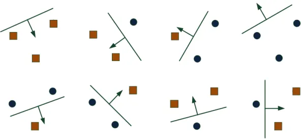
From a binary classification point of view, given n instances {x1, . . . ,xn} ⊂ Rm there are 2n ways to assign labels {−1,+1}to these instances. The instances

{x1, . . . ,xn} are said to be shattered by the model class H if, for all possible la-beling (2n cases), there exists at least one model from model class H which can classify the instances without any error. So the largest number of instances, which can be shattered by model classHis called the VC dimension of model class. More formally, based on the Vapnik and Chervonenkis, the VC dimension of model class

F is defined as follows:

maxn|X|

X ⊂ X, ∀g ∈ {−1,+1}X_{,∃h∈ F}

such that∀x∈X, h(x) =g(x)o .

By way of example, for a model class of linear functions with m variables, the VC dimension is equal tom+ 1. In Figure 2.1 all existing label assignments and corresponding separations are shown. If for a model class the VC dimension is un-bounded, then the VC dimension is infinite.

Loosely speaking, the VC dimension reveals the flexibility of a model class, the higher the VC dimension, the more flexible the model class is.

Figure 2.1: The illustration of shattering of three instances for model class linear functions with two variables

Structural Risk Minimization (SRM)

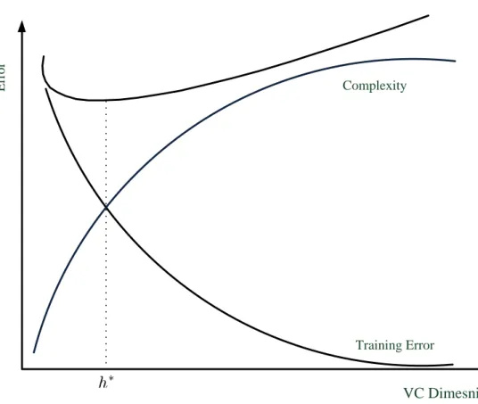
Under empirical risk minimization, two well-known problems can occur during the learning process. They are called, overfitting and underfitting. The overfitting prob-lem refers to when the capacity (complexity) of the learner clearly is higher than what is required. Likewise, the underfitting problem occurs when the capacity (complexity) of the learner is clearly lower compared to what indeed is needed. In order to overcome this problem, or let say, find the proper learner, Vapnik pro-posed the idea ofstructural risk minimization. Assume a family class of learners is given. Moreover, assume there is a possibility to order the learners based on their complexity, e.g. VC dimension. The main goal under structural risk minimization is to find a trade-off between the complexity of the learner and the goodness of generalization. More formally, the goal is to minimize

Remp(w) +λCP(w) ,

whereRemp is referred to the empirical risk, CP is referred to complexity penalty and finally λ is the trade-off parameter, which is determined empirically. In this regard, Vapnik proposed a bound to show a sound dependency between the risk and empirical risk given the VC dimension of the model.

Theorem 2.1 (Vapnik) AssumeHis the class of functions, with a VC dimension of

this distribution, the following inequality is valid with probability1−η. ∀h∈ H, R(h)≤Remp(h) + s v(log 2_vn+ 1)−log(n₄) n + 1 n . (2.4)

More formally, assume there is a possibility to order the hypotheses in hypothesis space as follows:

H0 ⊂ H1 ⊂ H2 ⊂. . .⊂ H ,

whereH=∪∞

i=0Hi. Moreover assume the VC dimension of eachHi is equal tovi. It is clear that

v0 < v1 < v2 < . . .

In general, choosing the hypothesis with a high VC dimension, due to high flexibil-ity reduces the empirical risk, while strengthening the overfitting problem. On the other hand, choosing the hypothesis with a low VC dimension reduces the flexibil-ity and hence increases the empirical risk. The core idea under SRM, is to find a trade-off (see Figure 2.2) between the complexity of the hypothesis and the quality of fitting in order to reduce the generalization error (R(h)) as much as possible. Note that based on the Vapnik theorem, choosing a hypothesis with high flexibility increases the second term in the right hand side of the equation (2.4).

VC Dimesnion Training Error Complexity E rr o r

Figure 2.2: The illustration of structural risk minimization, showing the trade-off between the complexity and the quality of fitting

The Concept of Regularization

In last part it was discussed that the higher flexibility of the learner increases the chance of the overfitting problem occurring. To this end, the core idea of SRM is to find a trade-off between the complexity of the learner and the quality of generaliza-tion in a proper way. To reduce the complexity of the learner, the parameters of the learner are restricted. To this end, the idea of regularization comes into play. The idea is to consider follwoing risk:

Rreg(f) =Remp(f) +λΩ(f) ,

wheref refers to a learner. In addition, the functionΩ(·)measures the regularity. HereRregis called regularized risk.

2.4 The Methods Derived from Inductive Principles

2.4.1

Linear Logistic Regression

In linear regression, given the dataD =(xi, yi) n

i=1 ⊂R

m_×

R, the goal is to find

β= (β1, . . . , βm)∈Rmand ∈R, such that

yi =β1xi1+β2xi2+. . .+βmxim+ ∀i, i∈ {1, . . . , n}

Herexi = (xi1, . . . , xim)∈Rm. Eachxij is called aregressororpredictor variable andyiis called a response.

The logistic regression modifies linear regression for the purpose of predicting (probabilities of) discrete classes instead of real-valued responses. To this end, the probability of the positive class (and hence of the negative class) is modeled as a linear function of the input attributes. More specifically, since a linear function does not necessarily produce values in the unit interval, the response is defined as a generalized linear model, namely in terms of the logarithm of the probability ratio:

log P(y = 1|x) P(y = 0|x) =ω0+ω>x , (2.5)

whereω = (ω1, ω2, . . . , ωm)∈Rmis a vector of regression coefficients andω0 ∈R

a constant bias (the intercept). A positive regression coefficientwi > 0means that an increase of the predictor variablexiwill increase the probability of a positive re-sponse while a negative coefficient implies a decrease of this probability. Besides, the larger the absolute value|ωi|of the regression coefficient, the stronger the influ-ence ofxi.

SinceP(y = 0|x) = 1−P(y = 1|x), a simple calculation yields the posterior probability πl df =P(y= 1|x) = 1 1 + exp(−ω0−ωTx) . (2.6)

Assume some observations are given, where thei.i.d.assumption is assumed. In order to find the proper generalization for given data, suitable parameters should be determined. This can be done by employing a maximum likelihood estimation. In the following analysis we will describe in more detail the maximum likelihood es-timation for a binary case. Assume the instancexand its labely ∈ {0,1}is given. Moreover assume a family of probability distribution P(·,·) is given. In general, the likelihood function for a binary class given an instancexand model parameters

ηis equal to:

P(y|x;η) = nP(y= 1 |x;η)oy·nP(y= 0|x;η)o1

−y

(2.7)

So now, assume some observations with corresponding responses are given, where the observations arei.i.d. as follows:

D=n(xi, yi)

on

i=1

⊂_Rm_×n_0,1o

For more than one instance, i.e.,xi, yi n

i=1, sincei.i.d. is assumed, the likelihood

function is formalized as follows:

L(η) =P(y|X;η) =P y1, . . . , yn|x1. . . ,xn;η =P y1|x1;η ×. . .×P yn|xn;η = n Y i=1 n P(yi = 1 |xi;η) oyi ·nP(yi = 0|xi;η) o1−yi , (2.8) whereX =nxi on i=1 ⊂_Rm _andy=

×

So the core idea of maximum likelihood is to find the parameters which maximize

L(η). Instead of maximizing the function in (2.8), it is more convenient to maxi-mize the logarithm of the function:

l(η) = logL(η) = logP(y|X;η) = n X i=1 n yi·logP(yi = 1|xi;η) + (1−yi)·logP(yi = 0|xi;η) o .

If the above function is given probability distribution be convex, then the optimal solution can be determined as follows:

∂l(η)

∂ηi

= 0 ∀i 1≤i≤p ,

wherep is assigned to the number of parameters. In this regard, the common ap-proach like Newton or quasi Newton can be used. In binary case, the log likelihood function is as follows:

l(ω, ω0) = logP(ω, ω0) = log n Y i=1 P(yi|xi;ω, ω0) ! = n X i=1 n yilogπ (i) l + 1−yi log 1−π_l(i)o , (2.9)

whereπ_l(i)is referred to in the equation in (2.6), where the instancexiis considered. In additionP(y(i) _{| x}(i)_{;ω, ω}

0) = π (i)

l

y(i)

. It is not difficult to check that the log likelihood function in (2.9), has a negative semidefinite Hessian matrix [15, 96]. Therefore, the function −l(ω, ω0) it is a convex function and to find the optimal

solution the usual methods like gradient descent or the Newton method can be em-ployed. For the Newton method, the optimal solution is as follows:

ω(n+1) =ω(n)−H−1∇ω −l(ω)

,

whereH and∇are referred to the Hessian matrix and gradient respectively. Furthermore, in order to establish a monotone learner, considering the linear logistic regression as a base-line, the following optimization problem is taken into account:

max ω,ω0 n X i=1 yilogπ (i) l + 1−yi log 1−π_l(i) (2.10) s.t. ωi ≥0 ∀i∈ {1, . . . , m} (2.11)

The constraints in (2.11) indeed assure the monotonicity for the linear logistic re-gression. The objective function in (2.10) is still convex, although beside some constraints exist. To this end, Lagrange optimization can accomplish the optimiza-tion problem.

2.4.2

Margin Maximization Principle

In this section, the basic idea of a large margin approach, namely the linear margin, is presented. Assume some labeled instances, which are supposed to bei.i.d. given as follows:

D=n(xi, yi)

on

i=1

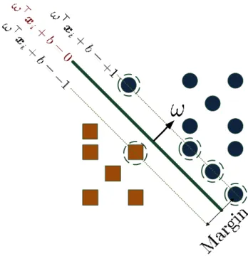
The labels {−1,+1}, can be considered as negative and positive classes respec-tively. The labeled instances are separable by a hyperplaneω∗ ∈_Rm _{and intercept}

b∈_R, if the following inequality is valid for all labeled instances:

∀i 1≤i≤n yi·

hω∗,xii+b

≥1 . (2.12)

In spite of this formulation, the instances with propertyhω∗,xii+b ≥ 1, belong to class +1, and the instances with property hω∗,xii+b ≤ −1 belong to class

−1. Accounting for the fact that there are infinite hyperplanes, which can satisfy the above inequality, this reveals that there is a great deal of flexibility for existing solutions. To cope with this flexibility, which certainly contributes to the overfitting problem, Vapnik proposed to use the idea of SRM. The core idea is to find a trade-off between the goodness of generalization and complexity of model. To this end, he proposed the following risk:

n X i=1 lyi,hω,xii +C||ω||2

Here l is the loss function and C is the trade-off parameter. Since we assumed that the instances can be classified by a linear hyperplane, it can be concluded, a set of hyperplanes exist{ωq}q∈Q, where for all q ∈ Q, Pn_i=1l(yi,hωq,xii) = 0. Therefore the problem boils down to minimizing the following term:

C||ω||2

with additional constraints

yi·

hω,xii+b

≥1 .

More formally the hyperplane can be determined as follows:

min ω,b 1 2||ω|| 2 s.t. yi· hω,xii+b ≥1 ∀i∈ {1, . . . , n}

This in essence is a quadratic programming optimization. In the light of above notations, the set ofsupport vectorscan be determined as follows:

( xS ∈ D |hω ∗ ,xSi+b|= 1 ) ,

whereω∗ is the solution of the optimization problem above. The vectorω∗ is also called thedecision boundary. In this case, thedecision boundaryis linear, however it can be quite non-linear. Then following, discuss in greater detail how to construct non-linear decision boundaries.

Figure 2.3: The illustration of separation of two classes by hyperplanehω,xi+b= 0. The objects on boundary, which showed by dot circles, called the support vectors.

In Figure 2.3, the position of hyperplane is shown and as well the support vec-tors. Since the above equality holds for support vectors, the distance between sup-port vectors and hyperplane can be computed as follows:

d(xS,P) = ω>xS+b ||ω|| = ±1 ||ω|| , (2.13) where_P = n

x ∈ _Rm _{| hω,xi+b = 0}o_{. Therefore, the magnitude of margin is} equal to_||ω2_||, and hence the solution to the above constrained optimization problem,

is the hyperplane, which maximizes the distance between the instances of two dif-ferent classes.

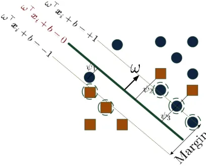
So far the assumption was, that the instances are linearly separable. One may also consider the case, in which the instances are not linearly separable, although the goal is to separate them by a linear hyperplane. This case is addressed as a soft margin. The core idea is to allow the classifier to make some mistakes, albeit as low as possible. In Figure 2.4 the idea is illustrated. This idea is again referred to as the structural risk minimization. To this end, assume the loss function is given. Then

Figure 2.4: The illustration of separation of two classes by soft marginhω,xi+b = 0. The objects on boundary, which showed by dot circles, called the support vectors.

the structural risk can be formulated as follows:

n X i=1 l(yi,hω,xii) +C||ω||2 = n X i=1 ψi +C||ω||2 .

The first term in the second equation, indeed, is considered for mistakes. Hence the linear soft margin can be formalized as follows:

min ω,ψ,b nXn i=1 ψi+ C 2||ω|| 2o s.t. yi· hω∗,xii+b ≥1−ψi ∀i∈ {1, . . . , n} ψi ≥0 ∀i∈ {1, . . . , n}

This is again a constraint optimization problem, and the optimal solution can be found by quadratic programming optimization.

2.4.3

Kernel Methods

It is apparent that if the instances are not linearly separable, then linear SVM can-not solve the problem properly, i.e., some instances are miss-classified. In order to prevent miss-classification, the basic idea is to transfer the data (instances) to an up-per space, of course with higher dimensionality, where the labeled instances can be separated linearly without any mistake. To this end, the core idea is to use kernels which can model the non-linear decision boundaries.

Before going into detail, we shall introduce some preliminaries. Assume the functionk(·,·)on domainX × X is defined as follows:

k :X × X →_R

(x,x0)7→k(x,x0) .

In order to establish the concept of the kernel, the following definitions and nota-tions are needed as taken from “Kernel methods in Machine Learning” by Hofmann et al. in [57].

Definition 2.1 (Gram matrix) Given a function k(·,·) and inputs x1, . . . ,xn ∈

X ⊂_Rm_{, then×nmatrix}

K :=k(xi,xj)

ij

Definition 2.2 (Positive definite matrix)A realn×nsymmetric matrix Kij

satis-fying

X

i,j

hihjKij ≥0

for all hi ∈ R is called positive definite. If equality only occurs for h1 = . . . =

hn= 0, then we shall call the matrix strictly positive definite.

Definition 2.3 (Positive definite kernel)LetX ⊂_Rm_{be a nonempty set. A function}

k :X × X →_Rwhich for alln∈_N,xi ∈ X, i∈ {1, . . . , n}gives rise to a positive

definite Gram matrix is called a positive definite kernel. A functionk:X × X →_R

which for all n ∈ _N and distinct xi ∈ X gives rise to a strictly positive definite

Gram matrix is called a strictly positive definite kernel.

Theorem 2.2 (Mercer’s Theorem) A symmetric function k(·,·) is a kernel if and

only if for any finite sampleS = {x1, . . . ,xn}the Gram matrix for S is positive

semidefinite.

If for a given kernel k(·,·), there is a mappingϕ : _Rm _→

Rp such that for all

x,x∗ ∈ _Rm_{, k(x,x}∗_{) = hϕ(x), ϕ(x}∗_{)i, the map ϕ(·) is called feature mapping}

with respect to the kernelk(·,·).

Givenntraining examplesxi n

i=1the optimal weights for a kernel is computed

by the so-called dual form[107]. The setting in a large margin case is called the

primal form. In fact from theprimal form, the dual form can be derived [87]. So in this case, the goal is to findα={αi}ni=1parameters, which minimize the following

objective function under constraints:

min α ( 1 2 n X i=1 n X j=1 yiyjαiαjk(xi,xj)− n X i=1 αi ) s.t. n X i=1 yiαi = 0 0≤αi ≤C ∀i, i∈ {1, . . . , n}

HereCis a typical SVM trade-off parameter. This problem actually can be solved by quadratic programming (QP), which givenninstances has a computational com-plexity ofO(n3). Interestingly, from α = (α1, . . . , αn)and training examples, ω can be computed as follows:

ω=

n

X

i=1

αiyiϕ(xi) ,

where ϕ(·) is the feature mapping corresponding to the kernel. In the following discussion, the kernels used in this thesis are introduced.

Polynomial Kernel

Letx,ybe two elements in_Rm. The polynomial kernel is defined as follows:

k(x,y) = hx,yi+λd ,

whered∈_Nis the degree of polynomial kernel and alsoλ∈_R. This corresponds to the feature mapϕ(·)including all monomialsxi1

1 . . . ximm whereij ∈N,Pmi=1ij =s

and0≤s≤d. Ford= 1it is called the linear kernel.

Gaussian Kernel (RBF)

Letx,ybe two elements in_Rm. The Gaussian kernel given parameterσis defined as follows: kσ(x,y) = exp −||x−y|| 2 2 2σ2 ,

This kernel is also called the radial basis function (RBF).

2.5 Monotone Classifiers

The problem of monotone classification has received increasing attention in the machine learning community in recent years [7, 29, 35], despite having been in-troduced in the literature much earlier [11]. Meanwhile, several machine learning algorithms have been modified so as to guarantee monotonicity in attributes, includ-ing nearest neighbor classification [33], neural networks [91], decision tree learninclud-ing [10, 85], rule induction [29], as well as methods based on isotonic regression [22] and piecewise linear models [28]. From a monotone learning point of view, specifi-cally for classification purpose, the monotone classifiers are trained in a way that the learned classifiers satisfy monotonicity properties. In general, monotonicity means

that by increasing the magnitude of attributes jointly or separately, the correspond-ing class also increases or at least stays at the same level. More precisely, assume the classifier is given as follows:

CL:X1×. . .× Xm → Y ={−1,+1} ,

whereX1×. . .× Xm ⊆ X ⊂Rm. The classifierCL(·)is a monotone classifier, if

∀xi,xj ∈ X s.t. xi xj then CL(xi)≤CL(xj) .

This definition can be extended to the ordinal classes, where there is a total order between classes. More concretely, assume the classesY = {y1, . . . , yk} with the following order are given:

y1 ≺y2 ≺. . .≺yK . Note that, yi

n

i=1 are not necessarily real numbers. In that case the above

definition can be extended as follows:

If xi xj then CL(xi)CL(xj) .

It is worth mentioning that usually enforcing monotonicity to specific model can be accomplished in light of extra constraints [67, 98]. For instance, every linear SVM with positive parameters forω is a monotone classifier. Needless to say, it is not always possible to enforce the monotonicity to an arbitrary model.

3

The Choquet Integral as an Aggregation

Function

In this chapter, the main ideas of Multi Criteria Decision Making (MCDM) and aggregation functions are presented. The aggregation functions are mostly used in theMulti Criteria Decision Making community. Loosely speaking, the task in multi criteria decision making is to select an object or an action between several alternatives. In this regard, each object or action can be characterized by its proper-ties. Ultimately such properties can be aggregated, and the final decision (selection, ranking) is made. This chapter begins by giving the core ideas in multiple criteria decision making. Then the aggregation functions as powerful tools in MCDM are introduced in 3.1.3. Specifically the Choquet integral as an aggregation function in Section 3.4 is presented and its properties will be described. As it has been men-tioned in introduction of thesis, the Choquet integral provides sound information in terms of interpretation. This issue is addressed as well in Section 3.6 in more the detail .

3.1 Multiple Criteria Decision Making

3.1.1

Introduction

To the best of our knowledge the initial idea of MCDM comes from philosophy, where the problem was to evaluate a premise by itsproandcontrareasons [36]. In this regard, the pro (advantages) and contra (disadvantages) reasons were weighted, and finally the weights were compared. If the weights of advantages compared to the weights of disadvantages were larger, the premise would be accepted, otherwise it would be rejected. In fact, the issue was to select an alternative among of several alternatives, where every alternative can be assessed by its advantages and disad-vantages. Generally, the selection of one alternative among all alternatives is not always a trivial task. The basic reason is, that it is quite rare that an alternative can cover all advantages, whereas it does not have any disadvantage. From this perspec-tive, the task in MCDM is to rank the alternatives in a preferable way. This chapter starts by an simple example to give the main idea of MCDM:

Assume a company wants to employ a programmer. Since the company is op-erating in the U.S. and China, it needs a person, who is proficient in a foreign language. Also70%of the projects are done usingJava,30%usingC+and know-ing SQL is preferable. Finally since the company faces complex problems, more educated employees are preferred. In addition, the company would not like to pay more than60k$ as salary to the employee. Accordingly every alternative can be described as a member of the following Cartesian product:

n

P({Eng.,Chin.})o×nP({Java,C+,SQL})o×nB.Sc.,M.Sc.,PhD

o

×nM,L

o ,

wherePis assigned to the powerset. HereMstands for more than60k$andLstands for less than60k$income. Note that here an empty set means the candidate cannot satisfy any preconditions regarding the specific condition. Needless to say, every alternative expects different amounts of income with respect to his/her qualifica-tions. The task here is to find a programmer who can satisfy as much as possible the prerequisites and moreover expects an income less than60k$as a salary.

3.1.2

General Idea

MCDM has been received considerable attention, especially from 50 years ago. This is indeed a subfield of operations research, which attempts to make a proper

choice among the given choices or to find the proper ranking/sorting among of the given choices. From an application point of view, the MCDM is used extensively in banking [6], transportation [27], urban management [113], energy and resource management [72], economy [71], energy planning [32] and financial management [23]. The task in MCDM can be summarized as choosing an alternative among given alternatives or sorting the alternatives. This task can be quite complex and confusing due to the fact that, every alternative can cover the benefits partially, i.e., usually an alternative cannot fully satisfy all expectations. Specifically in real applications, usually the criteria are conflicting, namely, increasing the satisfaction of certain criterion leads to decrease in the satisfaction of another criterion. In this regard, there is a need to make a choice in a transparent and consistent way. In general, every MCDM can be described by the following components:

• Alternative: An alternative is an object or an action which has a potential to

be chosen.

• Criteria:In order to evaluate each alternative and to make them comparable,

each alternative is characterized by some predefined criteria. Note that all alternatives are characterized by the same criteria.

• Make a Decision: Given the alternatives characterized by criteria, the

deci-sion is made by evaluating the alternatives and giving them scores, and ul-timately by choosing an alternative, sorting the alternatives or ranking the alternatives (total or partial) among several alternatives.

Therefore, regarding the above definitions, given the set of criteria

C ={c1, . . . , cm}each alternative can be evaluated as follows:

a= (a1, . . . , am) ,

where ∀i,1 ≤ i ≤ m, ai = fi(a). The function fi(·) is called the evaluation function w.r.t the criterionci, and indicates how high the alternative a can satisfy the criterionci. Commonly it is assumed that the range of the evaluation function is[0,1]. 0means the alternative cannot satisfy anything regarding criterionciand1 means the alternative satisfies perfectly the criterionci. Hence,

a = (a1, . . . , am) = f1(a), . . . , fm(a)

In order to make a choice or rank the alternatives, the existing methods in literature can be divided into three main sub-methods:

Outranking methods: The main idea in outranking methods is to define a pref-erence relation (partial order) of alternatives in a pairwise manner. More precisely

A≺B, implies the alternativeBis at least as good as the alternativeA. To this end, the core idea is to consider the criteria which support the assertion (A ≺ B) and the criteria which are against this. The initial idea has been proposed by Bernard Roy [86]. Multiattribute utility: The multiattribute methods usually consider the classical aggregation functions (we will describe the aggregation functions in the next section) and assign real numbers to each alternative. Therefore, they produce a total order given alternatives. Non classical methods: Finally the non-classical approaches mainly covered in the scholarly literaturedecision rules[55] andfuzzy integrals[50].

In this regard, while several well established methods such as ELECTRE (elimina-tion and choice expressing reality) [37], PROMETHEE (preference ranking orga-nization method for enrichment of evaluations) [18], TOPSIS (technique for order preference by similarity to ideal solution) [82, 112] and the MUTA (multi attribute utilities theory) [34] are counted as classical approaches, the aggregation functions underlying fuzzy measures are taken into consideration as a non-classical approach [42, 36]. In the following sections, these kind of aggregation functions will be de-scribed more in the details. Before continuing the topic, a new notation should be introduced.

So far the term attribute(s) was mentioned to characterize the feature space. Ba-sically every instance is characterized by some given attributes. We shall make a distinction betweenattribute andcriterion. From a MCDM point of view, criteria characterize the decision space. Every criterion is not a number, however, for each instance the evaluation of each criterion, namely, how good the alternative can sat-isfy specific criterion, is computed by its evaluation function (real value function). The term “criterion” is indeed often used in the decision making literature, where it suggests a monotone “the higher the better” influence. In the light of this definition, this fact comes down, that the higher the criterion, the higher the benefit is. Note that from now to the end of this thesis, the set of criteria are shown as follows:

C =nc1, . . . , cm

o ,

wheremis the number of criteria.

3.1.3

Aggregation Functions

As mentioned several times, one of the powerful tools from a decision making point of view is an aggregation function. The main duty of aggregation functions is to ag-gregate all advantages and disadvantages together and finally deliver them as a real (positive) number. Before going into details, we shall introduce the definition of aggregation functions.

Formally a functionA : [0,1]m _{→[0,1]is an aggregation function if it satisfies} the following conditions [21, 51]:

• monotonicity:∀ai,aj ∈[0,1]m, ifai ≺aj thenA(ai)≤A(aj)

• Unanimity:∀a= (a, . . . , a)∈[0,1]m_{, A(a, . . . , a) =a}

The second condition immediately boils down to the following equalities:

A(0, . . . ,0) = 0

A(1, . . . ,1) = 1

An aggregation function is symmetry, if for any permutationσ on{1, . . . , m},

A(a1, . . . , am) =A(aσ(1), . . . , aσ(m)).

In the following some important aggregation functions are presented:

Definition 3.1 (Weighted Mean): Given the weights ω = (ω1, . . . , ωm), where

ωi ≥0and

Pm

i=1ωi = 1, the weighted mean operator is defined as follows:

W M(a1, . . . , am) = m

X

i=1

ωiai .

Definition 3.2 (Ordered Weighted Averaging): Given the weightsω= (ω1, . . . , ωm),

whereωi ≥0andPm_i=1ωi = 1, and moreover a decreasing permutationπ(aπ(i) ≥

aπ(i+1) for a givena), the OWA operator is defined as follows:

OW A(a1, . . . , am) = m

X

i=1

ωiaπ(i) .

In the following sections, we give the preliminaries for introducing an important aggregation function underlyingfuzzy measure.

3.2 The Choquet Integral as an Extension of Lebesgue

Integral

Henri Lebesgue proposed the extension of the Riemann integral, where instead of considering the length of an interval as the weight, he presented the concept of measure to construct the integral. Such measures have a specific property, namely, countable additivity. More precisely, the measure of union of two distinctive sets is equal to the sum of measures of each set. Later on Gustave Choquet proposed the generalization of the Lebesgue integral in a way that he suggested corresponding measure can be non-additive measures. More formally, assume functionf : S →

R is measurable with respect to measureν. The Choquet integral for function f respect to measureνis defined as follows:

(c) ˆ S fdν := ˆ ∞ 0 ν{s |f(s)≥x}dx+ ˆ 0 −∞ h ν{s |f(s)≥x}−ν(S)idx

It is worth mentioning that ifνis aσ-additive measure, the above definition comes down to the Lebesgue integral.

3.3 Fuzzy Measures

Before describing the details, some preliminaries about non-additive measures and especially fuzzy measure are introduced. As mentioned earlier, the crucial differ-ence between the Choquet integral and the Lebesgue integral is the type of measure.

3.3.1

Non-Additive Measures

In this section the properties of non-additive measures are investigated in greater de-tail. Generally, non-additive measures do not satisfy the additive property. Hence, non-additive measures obviously are more flexible and can model a larger class of measures as well. In the following discussion, the main properties of such kind of measures are introduced.

LetC ={c1, . . . , cm}be a finite set of criteria andµ(·)a measure2C →[0,1]. For eachA⊆ C, we interpretµ(A)as theweightor, say, theimportanceof the set of elements A. As an illustration, one may think of C as a set of criteria (binary features) relevant for a job, like “speaking French” and “programming Java”, and of µ(A) as the evaluation of a candidate satisfying criteria A (and not satisfying

X\A).

A standard assumption of a measureµ(·), which is at the core of probability the-ory is additivity:µ(A∪B) = µ(A) +µ(B)for allA, B ⊆Xsuch thatA∩B =∅. Unfortunately, additive measures cannot model any kind of interaction between el-ements: Extending a set of elementsAby a set of elementsB always increases the weightµ(A)by the weightµ(B), regardless ofAandB. Suppose, for example, that the elements of two setsAandBarecomplementaryin a certain sense. For instance,

A={French,Spanish}andB ={Java}could be seen as complementary, since both language skills and programming skills are important for the job. Formally, this can be expressed in terms of a positive interaction: µ(A∪B) > µ(A) +µ(B). In the extreme case, when language skills and programming skills are indeed essential,

µ(A∪B)can be high althoughµ(A) =µ(B) = 0(suggesting that a candidate lack-ing either language or programmlack-ing skills is completely unacceptable). Likewise, elements can interact in a negative way: If two setsAandB are partlyredundant

orcompetitive, then µ(A∪B) < µ(A) + µ(B). For example, B = {Java}and

C ={C,C#}might be seen as redundant, since one programming language does in principle suffice.

3.3.2

Fuzzy Measures and their Möbius Transforms

As mentioned before, non-additive measures are characterized by different proper-ties. Among all non-additive measures, there is a specific kind of measure called

fuzzy measures. They have a unique property called monotonicity. This property guarantees, that the measure of each subsets of a setS have the magnitude smaller than (or equal to) the measure ofS ⊂C.

Definition 3.3 (Fuzzy measure) Let C = {c1, c2, . . . , cm} be a finite set. A

dis-crete fuzzy measure (also called capacity) is a set functionµ : 2C _{→ [0,1]which}

is monotonic (µ(A) ≤ µ(B) for A ⊆ B ⊆ C) and normalized (µ(∅) = 0 and

µ(C) = 1). A fuzzy measureµis called additive ifµ(A∪B) = µ(A) +µ(B)for allA, B ⊂ Csuch thatA∩B =∅. Obviously, in the case of an additive measure,

µ(A)is simply obtained as follows [95]:

µ(A) =X

i∈A

µ({i}) (3.1)

Definition 3.4 (Möbious transform) The Möbius transform mµ of a fuzzy

mea-sureµis defined as follows:

mµ(A) =

X

B⊆A

(−1)|A|−|B|µ(B)

for allA⊆C.

A useful property of the Möbius transform, that we shall exploit later on for learning the Choquet integral, it allows for reconstructing the underlying fuzzy mea-sure: µ(B) = X A⊆B mµ(A) for allB ⊆C.

3.3.3

Monotonicity Constraints

Given an arbitrary measureµ : {c1, . . . , cm} → [0,1], with additional assumption

µ({c1, . . . , cm}) = 1, one natural question is, whether the measureµ(·)is a fuzzy measure or not. In order to check this issue, the basic idea is to check the following inequalities:

µ(L)≤µ(K) ∀L, K L⊂K ⊆ {c1, . . . , cm} .

Since each subset of{c1, . . . , cm} is compared with all its subsets 3m −2m con-straints must be checked,

m X i=1 m i (2i −1) = m X i=1 m i 2i− m X i=1 m i = 3m−2m .

Fortunately, the last two constraints can be represented in a more compact way, exploiting a transitivity property:

µ(L)≤µ(K) ∀L, K L⊂K ⊆ {c1, . . . , cm}, |K|=|L|+ 1 .

Respectively in terms of Möbius transform the above constraints can be reformu-lated as follows: X B⊆A\{ci} mB∪ {ci} ≥0 ∀A⊆C, ci ∈C

This representation reduces the number of constraints tom2m−1_{, which, despite still}

being large, is a significant reduction in comparison with the original formulation.

3.3.4

k

-additivity

There is a close connection between a fuzzy measure and the Möbius transform; given a fuzzy measure the so-called Möbius transform can be constructed con-versely as well. From a computational point of view, there is a complexity re-duction, so that instead of considering all values for the Möbius transform only a subset of values are taken into account. This reduction is calledk-additivity, where

kis referred to the level-complexity.

Definition 3.5 (k-Additivity) A fuzzy measureµ is said to bek-order additive or

simplyk-additive if k is the smallest integer such thatm(A) = 0for all A ⊆ C

with|A|> k.

Thus, while a Choquet integral is determined by2m _{coefficients in general, the}

k-additivity of the underlying measure reduces the number of required coefficients to at most k X i=1 m i .

3.4 The Discrete Choquet Integral

In previous section, the general idea of the Choquet integral was introduced. In this section we restrict ourselves to discrete cases, where the measureν acts solely on finite domain in terms of cardinality.