A Globally Consistent Stress Testing Approach

(1)

Research in Economics and Management ISSN 2470-4407 (Print) ISSN 2470-4393 (Online) Vol. 4, No. 3, 2019 www.scholink.org/ojs/index.php/rem

Original Paper

A Globally Consistent Stress Testing Approach

Colin Ellis1*

1_{Department of Economics, University of Birmingham, Birmingham, UK}

* _{Colin Ellis, Department of Economics, University of Birmingham, Birmingham, UK. E-mail:} [email protected]

Received: April 18, 2019 Accepted: May 31, 2019 Online Published: June 24, 2019 doi:10.22158/rem.v4n3p153 URL: http://dx.doi.org/10.22158/rem.v4n3p153

Abstract

This paper describes an approach for stress testing banks that is consistent across economies and geographies, in contrast to common “macro scenario” driven approaches. The latter would require economic scenarios to be both equally likely (in a probabilistic sense) and equally stressful (in a conditional loss sense) across countries in order to be comparable. The paper proposes a three-pronged approach for stressing bank solvency, which incorporates recalibrating pre-crisis Basel capital assumptions, adapting the BIS “expected shortfall” approach for securities, and using granular data for income haircuts. Loan losses are quantified using a simple “multiples” approach, starting from expected outcomes, which is derived from the pre-crisis Basel technical proposal. The approach is practical, can be more granular or conducted at a high level, depending on data availability, and offers a simple way for regulators, investors or risk assessors to compare and contrast stresses in different banking systems. Of the eight bank defaults recorded globally during 2017, this approach would have given a better “rank ordering” for seven of them, indicating the approach adds value to traditional solvency metrics. Keywords

banks, stress tests, solvency, capital, asset quality

1. Introduction: Different Stress Testing Approaches

Since the 2007/8 financial crisis, stress testing has become a key tool for bank planning and regulatory purposes. However, there are a number of different approaches to stress testing. Prior to the 2007-8 financial crisis, implicit stress tests embedded in banks’ internal capital calculations were commonly used to inform banks’ capital buffers. But with many bank failures exposing these as inadequate ex post, interest in stress tests has intensified over the past decade. Key international regulatory guidance on stress testing was provided by the Basel Committee on Banking Supervision (BCBS) in 2009 (BCBS, 2009); and both the Board of Governors of the Federal Reserve System (2015) and the European

(2)

www.scholink.org/ojs/index.php/rem Research in Economics and Management Vol. 4, No. 3, 2019

154

Published by SCHOLINK INC.

Banking Authority (2014) have prescribed recent large-scale regulatory stress tests in the US and the European Union.

A key feature of these exercises was to shift away from previous “value at risk” (VaR) approaches. VaR analysis can offer some substantial advantages, including its practical viability and conceptual attractiveness (Kupiec, 1998) and the ability to contrast multiple models and calibrations (see for example Alexander and Sheedy, 2008). But with its decline, stress tests instead became increasingly reliant on a form of scenario analysis: taking unexpected (downside) macro scenarios and estimating how those impact, via loan and securities losses, on bank capital. Lopez (2005) was one of the first to note that this mechanism would link losses to “specific and concrete” events; Jokivuolle, Virolainen and Vähämaa (2008) is one early post-crisis example of macro-driven stress testing. The popularity of these macro-driven tests extended to regulators, with some policymakers arguing they should replace the previous “Internal Ratings Based” (IRB) approach to risk-weighted capital (Tarullo, 2014). However, there is no consensus here; Borio, Drehmann and Tsatsaronis (2012) note that macro-driven stress tests are not suitable as early warning devices and would benefit from complementary information.

Concerns have also been raised about the appropriateness of the modelling framework that links macroeconomic data to bank loss rates. To start with, these frameworks were often similar to classic macro modelling and hence focused on the middle of the distribution of losses (see for example Bunn et al., 2015; and Miani et al., 2012), rather than the tail. In some instances, researchers recognized this by proposing adjustments to estimated models, for instance in Buncic and Melecky (2012). However, regulators may also have responded by picking unusually stressful scenarios in their macro-based stress tests (Ellis, 2017). More recently, there has been renewed focus on flexible models that allow these relationships to change as the analysis moves into the tail of the distribution (Covas, Rump, & Zakrajsek, 2013). These quantile models, as introduced by Koenker and Hallock (2001), may offer a better guide to stressed outcomes, but they are not yet widely employed.

However, macro-driven stress tests encounter further challenges when there is a need to compare and contrast banks in different regions or jurisdictions. Applying the same degree of stress across countries is far from simple for typical macro-driven stress tests. An assumed recession that decreases GDP by, say, 3% may not be as probable today in the US as in Indonesia; conversely, an equally probable scenario (say, with a 10% probability) may well entail a deep recession in one country and a more mild slowdown in another. Similarly, tying all countries to a single shock that is transmitted globally will not be equally stressful for every country that is affected, as the exposure to the shock and the nature of the transmission mechanism will vary from country to country.

In light of these challenges, the approach described in this paper is deliberately different: and, consequently, is not intended to be directly comparable with macro-driven stress tests. In large part, this reflects the aims and of and context in which the approach was developed, with comparability and consistency across different countries and regions being more important than country-specific risks or

(3)

www.scholink.org/ojs/index.php/rem Research in Economics and Management Vol. 4, No. 3, 2019 scenarios (which by their very nature will be heterogeneous). However, these discrepancies do not necessarily imply differences in judgments about the relative strength or viability of a bank under stressed conditions. Ultimately, as with other stress tests, this approach still aims to analyze banks’ resilience under stressed conditions against a group of peers, in order to uncover potential weaknesses in the financial system.

This paper therefore describes an approach to stress testing that does not rely on downside macroeconomic scenario and, unlike most macroeconomic-driven stress tests, allows consistency and comparability of results across banks within a jurisdiction and across different jurisdictions. The rest of this paper describes each of the components in this approach that determine the stressed capital ratio. Section 2 deals sequentially with loan losses, stressing banks’ income, and an approach for security losses. Section 3 then shows the results of this approach for over 70 banking systems, highlighting those more vulnerable to stressed conditions and those more resilient. Finally, the discussion in Section 4 concludes.

2. Method

2.1 Loan Losses: Starting from the Expected Case

While point forecasts represent the average or most likely outcomes given a set of macroeconomic and industry conditions, stress tests literally represent unexpected developments. As such, it is possible to draw parallels between the two: and indeed to express stressed loss rates or stressed default rates as a “multiple” of expected rates. The higher the multiple, the bigger the increase from the expected to the stressed case.

In order to exploit this link – in the context of loan losses – the analysis needs to start from an expected case. Given data limitations in many countries, one simple approach is to focus on system-level trends in asset quality, as measured by the aggregate Non-Performing Loan (NPL) ratio. As shown in past work (see for instance Buncic & Melecky, 2012, and Moody’s, 2014a and 2014b), it is possible to model system-level trends in asset quality and default rates based on expected developments in the economic and financial environment, where macroeconomic data – such as real GDP, unemployment, inflation, and the exchange rate – are used to obtain forecasts for the NPL ratio.

However, econometric techniques and models differ. In general, NPL series tend to be relatively short for most banking systems (most of which are in emerging or developing economies); as a consequence, panel models may be needed to exploit cross-country patterns in the linkages between NPLs and macroeconomic variables. Wherever there is greater data availability, country-specific models can be estimated. But in either instance, the outcome from this approach is a set of projections for the aggregate or total NPL ratio in the banking system. In turn, this can be transformed into a Probability of Default (PD) given an assumption about the write-off rate of NPLs, using a simple “law of motion” approach (see Buncic & Melecky, op cit).

(4)

156

System-level profiles for NPL ratios can easily be transformed into NPL ratios – or PDs – for individual loan types, provided either disaggregated data on these categories are available, or assumptions are applied about the distribution of loans and asset quality. In some instances where data are more plentiful, it is possible to build specific forecasting models for individual loan types.

One important point here is that – by and large – input data are not adjusted for idiosyncratic factors above and beyond routine adjustments. Several private agencies collect arrays of balance sheet and accounting data from rated issuers, which are then adjusted to provide standardized metrics across different geographies and jurisdictions (see for instance Moody’s, 2017). In principle, these input data should only be adjusted if there are clear and unambiguous grounds for doing so. For instance, an implicit assumption is often that underwriting standards are broadly consistent over time – or at least that any change is evident in metrics such as default rates or non-performing loans. This assumption is important because making sensible ad-hoc adjustments for as yet unobserved structural changes is difficult.

It is also important to note that the granularity of the data typically varies significantly from country to country and region to region. As such, simplifying assumptions are often needed. In the case of aggregate figures on, for instance, loan-to-value ratios, this implies that some banks in a system will be relatively “penalized” by using an average figure, while others will implicitly benefit. But provided the aggregates are broadly correct, these differences should average out across the system as a whole. Where assumptions are needed for granular loan loss rates, these can be linear or non-linear provided they are consistent with the aggregate loan profile. It is also likely that individual banks may well see different PDs within the same financial system, as a result of bank-specific factors such as the quality of underwriting. To the extent to which these factors are evident in differential default data, they can also be incorporated.

This approach can then be used to calculate default rates on different loan types – and for different banks – that are consistent with a central macroeconomic scenario. However, in order to calculate loan losses estimates of loss given default (LGD) are also required.

There is a rich body of literature around LGD estimates, including many loan-specific estimates. Based on a survey of over 70 such estimates, there can be considerable variability in the appropriate LGD, depending on the type of loan (see Figure 1). A simple starting point is to use the median estimates shown; but wherever more country-specific data is available, that can also be incorporated. Similarly, differences in Loan-To-Value (LTV) ratios can also inform different LGDs for residential and commercial property.

(5)

www. Sourc (2006 Davyd (1998 and H Memm Qi an 2.2 Th The b routin also b ensure equall institu The a unexp II. As risk w appro invari that lo expec nests (2005 The r propo .scholink.org/ojs/in ce: Author’s c 6), Bastos (201 denko and Fr 8), Felton and Hurt (1998), Ja mel et al. (201 d Yang (2007) he Role of Mul broad approac nely used by b be used to estim e that those st ly likely (in a utions and ban alternative pro pected (or stres s part of the g weights, the B oach that could

iance: this imp oan, and not o cted and unexp

an estimation 5). egulatory map osed by Merton ndex.php/rem Figure calculations ba 0), Brooks and anks (2008), D Nichols (2012 ang and Katao 11), Miroslav ), Wezel et al. (

ltipliers: Linki ch outlined ab banks and othe

mate the impa tressful macro a probabilistic nking systems. oposed here is ssed) losses, b uidance aroun Basel Commit d serve as a gu plies that the c on the portfolio pected losses a n of the entire pping implied n (1974), and Resea 1. Range of L

ased on: Arate d Cubero (200 Dermine et al 2), Grunert and oka (2013), Ja et al. (2006), M (2012). ing Baseline PD bove, linking er entities for p ct of non-cent scenarios wou sense) and eq s to construct y adapting som nd the “Interna ttee sponsored uide to banks (G capital require o that it is adde associated wit e distribution o in this researc as such depen arch in Economics a LGD Estimate en et al. (2004 09), Button et a l. (2006), Dre d Weber (2009 ang and Sheri

Moody’s (200 Ds to Stressed central macro planning and r tral outcomes, uld be compar qually stressfu t a simple me me of the regu al Ratings Bas d the developm Gordy, 2003). d for any give ed to. Using th th each credit of potential lo ch was derived ds on the prop and Management es by Loan Typ 4), Asarnow a al. (2010), Cha ehman et al. (2 9), Esaki and G dan (2012), Ji 00), Moody’s ( d PDs oeconomic sc regulatory pur like stress test rable, because ul (in a condit echanism for ulatory framew sed” (IRB) app

ment of a spe A key feature en loan should his framework exposure, bec osses: further d from a versio perties of the n Vo pe and Edwards ( alupka and Kop

2008), Eales a Goldman (200 imenez and M (2004), Powell enarios to cre rposes. In prin ts. However, it they would ne tional loss sen relating expec work first introd proach to calc ecific risk-fac e of this model d depend only k, banks could cause the mod details are pro on of the singl normal distribu Vol. 4, No. 3, 2019 (1995), BCBS pecsni (2009), and Bosworth 05), Felsovalyi Mencia (2007), l et al. (2004), edit losses, is nciple, it could t is difficult to eed to be both nse) across all cted losses to duced in Basel ulating banks’ ctor modelling l was portfolio on the risk of then calculate delling process ovided in BIS le asset model ution, which is S , h i , , s d o h l o l ’ g o f e s S l s

(6)

www. Publish assum could which The b (centr “mult with algebr Sourc The d are al be sm borrow are al is like In co robus The c can b impai Basel losses curve and h .scholink.org/ojs/in hed by SCHOLINK med to capture d be relaxed in h can again var broader perspec

ral) losses ban tiple” relations the degree of raic derivation Fig ce: BIS (2005) downward slop lready seeing h mall. When an wers is already ready likely to ely to be relativ ntrast, banks’ tly, and the dis convexity of th be quite sharp irments is likel approach ther s, for banks. O s implied by t ence can be ap ndex.php/rem INC. the change in principle. It al ry. ctive is that th nks face, and ship was entire f expected (ce ns are reported gure 2. Stress and author’s c pe of the curve high losses, th n economy is y likely to be r o be high. As s vely low, at le impairment r stance to a stre he multiple cur p when unex ly to be lower refore offers a One particularl the regulatory pplied to differ Resea value of a bor lso depends up his modelling a the unexpecte ely defined – i entral) loss: ill in Appendix 1 “Multiples” I calculations. es in Figure 2 he relative dist in recession, running at high

such, the dista ast compared w rates are likel ess scenario ma rves is consiste xpected losses r if the econom another means y appealing fe framework ar rent banking sy arch in Economics a 158 rrowers’ assets pon the correla approach can d ed (stressed) l f implicit – in lustrative mult 1. Implied by Ba has a simple i tance between

and real incom h levels. In the ance to an imp with a differen ly to be relati ay be relatively ent with the fac s first start t my is already in

of constructin eature of this a

re global in na ystems and cou

and Management s. However, th ation assumed define a relatio osses in the t the original B tiple curves a asel II Capital interpretation: the expected mes are fallin ese circumstanc

licit stress sce nt economy tha

ively low whe y high. ct that initial d o mount; but n recession. T ng unexpected approach is tha ature, as the o untries. Vo his distribution between differ onship between ail of the dist Basel calibratio are shown in F l Approach it implies tha and stressed o ng, financial d ces, banks’ im nario – a deep at is not alread en an econom deteriorations in t any acceler This simple ada

loss rates, or at, in principle original techni Vol. 4, No. 3, 2019 nal assumption rent borrowers n the expected tribution. This ons, and varies Figure 2. The

at, when banks outcomes may distress among mpairment rates per recession – dy in recession my is growing n asset quality ration in loan aptation of the stressed credit e, the multiple cal work was, n s, d s s e s y g s – n. g y n e t e ,

(7)

www.scholink.org/ojs/index.php/rem Research in Economics and Management Vol. 4, No. 3, 2019 In principle, these multiple curves can be used to generate stressed loss outcomes, obviating the need for a set of globally consistent macro scenarios for individual countries. However, they also suffer from obvious shortcomings, notably the poor performance of capital risk weights during the financial crisis. This suggests that the original asset risk models proposed by Basel need recalibrating. Properly assessing this would require estimates of pre-crisis expectations for credit losses, which are not readily available. But two simple proxies are easy to construct: the first is based on the assumption that expected losses were equal to the pre-crisis series average; for the second, we can assume that expected losses followed a random walk, implying they would be the same as realized losses in the previous year.

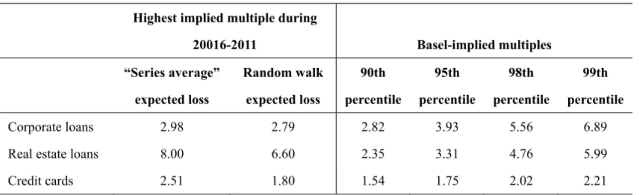
Armed with these pseudo “real time” estimates of expected losses, it is possible to examine what the actual loss outturns during the crisis implied in terms of multiples, compared with the original Basel calibrations. Table 1 presents results for the US, where data are most granular and coverage is good.

Table 1. US Banks’ Crisis Experience and Basel-Implied Multiples

Highest implied multiple during

20016-2011 Basel-implied multiples “Series average” expected loss Random walk expected loss 90th percentile 95th percentile 98th percentile 99th percentile Corporate loans 2.98 2.79 2.82 3.93 5.56 6.89

Real estate loans 8.00 6.60 2.35 3.31 4.76 5.99

Credit cards 2.51 1.80 1.54 1.75 2.02 2.21

Source: Federal Reserve and author’s calculations.

The results here suggest that the Basel models may not have been very misleading in the recent crisis for corporate loans, and to a lesser extent credit cards, depending on the implicit likelihood assigned to the financial crisis. The highest observed multiple for corporate loans, of 2.98, was well within the tail risks implied by the original calibrations. Unsurprisingly, the most obvious difference is for real estate, where the multiples observed during the crisis were much higher than the pre-crisis models suggested. But this offers an obvious recalibration approach: parameters from the original Basel specification can be adjusted until the implied multiples match the observed outcomes at some given percentile. For instance, given the implied multiple observed during the crisis was as high as 8 for US real estate loans, but the 99th Basel-implied percentile was only around 6, the Basel approach can be recalibrated to generate in higher multiples for real estate loans.

This approach therefore offers a simple but consistent mechanism for constructing stressed loss rates on different lending types across banks in different systems.

(8)

www. Publish 2.3 In Bank any s solven mitiga unaffe Howe develo period chang across chang sampl Sourc Using under repres that th would In pra sector these Furthe sampl region (inclu .scholink.org/ojs/in hed by SCHOLINK ncome Haircuts

stress tests are tress test relat ncy; the abili ating factor a ected by such ever, it is diffi

opments over d. In the absen ges in Pre Pro

s hundreds of ges in PPI and le of around 70 Fig ce: Moody’s (2 g these data, w rlying assump sentation of th he data captu d be possible t actice, changes

r risk and idios across countri ermore, it doe le of banks (co ns (advanced uding the sever

ndex.php/rem

INC.

s: Using the U e about more t tes to the trea ity to interna against emergi stresses, and m ficult to estima time. In part, nce of these re vision Income f banks each y d its componen 00 banks betw gure 3. Globa 2016b). we can estimat ption here is he true, unobse ure sufficient h to modify this s in PPI (and i syncratic risk. ies and over ti es not seem an ommercial, inv and emerging re recession in Resea Unconditional D

than loan losse atment of bank ally generate

ng stresses. A may fall as con

ate stable rela this reflects a elationships, ba e (PPI). Fortun year, allowing nts. Figure 3 p ween 2007 and al Distribution e income hair that the dat erved uncondit heterogeneity

distribution, d its components But, in the ab ime, this assum n unreasonabl vestment, deve g economies) 2009 and the arch in Economics a 160 Distribution es on credit po ks’ income. P capital, via r At the same t nditions deterio ationships betw a relative lack ank income is nately, some d g us to build u plots the distr 2015.

n of Two-Year

cuts for use in ta distribution tional distribut across and wi depending on w s) will reflect bsence of a mo mption provid le assumption elopment, univ and it includ uneven recove and Management ortfolios, howe Profitability is retaining earni time, it is unl orate. ween banks’ in of granular in stressed base data providers up a picture o ribution of two r Changes in B n stress tests, b n shown in tion of change ithin regions a what assumptio a range of fac del that can co des a simple an given that the versal banks; b des data throu ery thereafter).

Vo

ever. One key a key determ ings, can be likely that ear

ncome and m ncome data ov d on the distri collect inform of the global d o-year change Banks’ PPI based on tail o Figure 3 is es in PPI: that

and over time ons are deeme ctors, including onsistently acc nd practical wa e sample inclu big and small b ughout the ec . Vol. 4, No. 3, 2019 component of minant of bank an important rnings will be macroeconomic er a long time ibution of past mation on PPI distribution of s in PPI for a outcomes. The a reasonable is, we assume e. However, it ed appropriate. g country risk, count for all of ay to proceed. udes a diverse banks), across conomic cycle f k t e c e t I f a e e e t . , f . e s e

(9)

www.scholink.org/ojs/index.php/rem Research in Economics and Management Vol. 4, No. 3, 2019 Based on this assumption, the observed distribution can be used to generate income haircuts for banks, which can be applied in stress tests. In particular, depending on the desired degree of stress to apply – and, consistent with the multiples approach to loan losses, this can be defined as a percentile of the distribution – an income haircut that is consistent with the observed distribution can be employed. For instance, in a “1 in 25” stress test, the income haircut would be informed by the 4th percentile of the distribution of changes in PPI.

In practice, this approach can be employed for different components of banks’ income, such as net interest income and non-interest income, rather than focus on aggregate PPI. Importantly, however, income haircuts are not applied to trading income: this is covered under the securities stress approach, and hence would “double count” stresses if also applied here. Similarly, a simplifying assumption in several stress tests is that operating expenses are constant, and that the impact of management actions is limited to pre-announced measures. However, if these assumptions – or indeed the observed distribution of income changes – is not representative, then either the assumptions, or the distribution of income data, can be adjusted to inform different approaches. The main goal here is to demonstrate that the approach again offers a simple and consistent mechanism to consistently stress banks around the globe, based on the observed data.

2.4 Securities Losses: A Differentiated Approach

The third key component in this stress testing approach is to impose losses on banks according to their securities holdings. For many banks around the world, securities represent a relatively small component of the total balance sheet, compared with loans. But despite this, securities can play a significant role in stress tests.

In principle, there are three broad categories of securities holdings (and a residual “other” category). The first are securities that are Held To Maturity (HTM). In essence, banks will only realize losses on these securities if they default. The second are securities on the trading book (TRD). And the third are securities that are available for sale (AFS). Given the different nature of these three groups, a differentiated approach for stress testing is required.

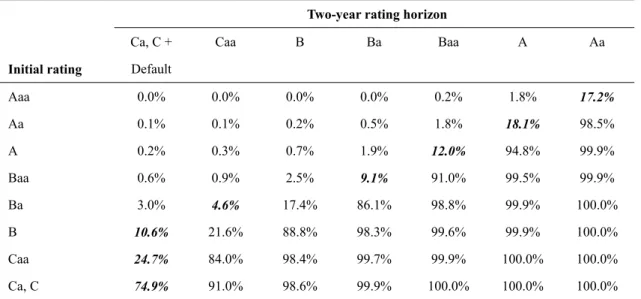
For HTM securities, where a published credit rating exists, it is simple to apply published loss rates associated with that published rating (see Moody’s, 2016a). However, in a stressed scenario there would likely be some deterioration in ratings from their pre-stress levels. This risk can be incorporated using published transition matrices for ratings. For instance, for a two-year stress, and again focusing on a “1 in 25” event, the 4th percentile of rating transitions can inform potential deteriorations in credit quality.

Based on published data, in this instance that would be broadly consistent with a three-notch rating downgrade; so a “1 in 25” stress for bank with bonds rated Baa2 (on Moody’s scale) would imply a downgrade to Ba2 (Table 2). This in turn corresponds to a published two-year (idealized) loss rate of 1.9%. Where published ratings are not available, benchmarks can be constructed based on close peers

(10)

162

or assumptions; for instance, that the average rating of corporate bonds held by a bank matches the average rating in the region or country where the bank is domiciled.

Table 2. Two-Year Cumulative Rating Transition Rates

Two-year rating horizon

Initial rating Ca, C + Default Caa B Ba Baa A Aa Aaa 0.0% 0.0% 0.0% 0.0% 0.2% 1.8% 17.2% Aa 0.1% 0.1% 0.2% 0.5% 1.8% 18.1% 98.5% A 0.2% 0.3% 0.7% 1.9% 12.0% 94.8% 99.9% Baa 0.6% 0.9% 2.5% 9.1% 91.0% 99.5% 99.9% Ba 3.0% 4.6% 17.4% 86.1% 98.8% 99.9% 100.0% B 10.6% 21.6% 88.8% 98.3% 99.6% 99.9% 100.0% Caa 24.7% 84.0% 98.4% 99.7% 99.9% 100.0% 100.0% Ca, C 74.9% 91.0% 98.6% 99.9% 100.0% 100.0% 100.0%

Note. Transition probabilities are cumulative from the left-hand column to the right-hand one. The rating category that nests a 4% cumulative downside outcome (consistent with a “1 in 25” stress) is shown in bold italics.

Source: Moody’s (2016c).

The treatment of securities on the trading book (TRD) should necessarily be different. In principle, these are not securities that banks will necessarily hold for long periods of time, so imposing large credit losses that may not crystallize for the bank may be inappropriate. At the same time, the trading book is affected by market risk in a much more immediate fashion than securities that are held to maturity. The process for stressing these securities is an adaptation of the “expected shortfall” approach outlined by the Basel Committee (BCBS, 2016). Essentially, this approach estimates loss rates on securities for a given holding period, which are calibrated using losses observed in a severe preceding year. Using past data for equity and bond indices that cover the global financial crisis in particular – which tends to represent the most severe 12-month period in recent history – loss rates for different types of securities can be calculated. Where data limitations are prohibitive and do not allow country-specific loss rates to be calculated, regional loss rates can be constructed, or loss rates from comparable countries can be used. Illustrative examples of loss rates are presented in Figure 4; further details on the expected shortfall approach are provided in Appendix 2.

(11)

www. Fi Sourc The th securi the ris Howe notch AFS incom In add appro action and o those Taken solven Howe positi and b 3. Str In pri corres time p are pr The ty at the down .scholink.org/ojs/in igure 4. Two-Y ce: Moody’s (2 hird category ities on the AF sk associated w ever, AFS bon

ing for stress o securities do me; they impac dition to the t oaches general ns, dividends a often rely on s outlined abov n together, the ncy metrics g ever, it is imp

ons will neces enchmarks tha ress Tests in A inciple, the str sponding to di periods; the de resented based ypical impact end of 2016, by near 8 per ndex.php/rem Year Stressed 2016c). of securities a FS book is ass with equity is nds are stress outlined earlier not impact on ct capital and e treatment of lo lly encompass and risk-weigh simple assump ve. ese assumption globally, and ortant to note ssarily respond at can inform ju Action: Identif

ress testing app ifferent percen egree and dura d on a “1 in 25” of this calibra the median ba rcentage points Resea d Loss Rates o

are those that sumed to follow best gauged u ed following r), since this b n net income, equity measure oan losses, pr ses a number hted assets. Th ptions; in this ns and method one that is n that no stress d to unexpected udgments abou fying Banks V proach outline ntiles in the ta ation of the st ” event, occurr ation on bank s anking system s (pp, from a s arch in Economics a on Securities f are Available w that of TRD using a market the HTM app better reflects c

, but are accu es when realize e-provision in of other assum hese are detaile

stress testing ds form a con not dependent s test provides d developmen ut the banks’ r Vulnerable to S ed above can b ails of the ass tress can vary. ring over a two solvency metri would see its starting level o

and Management

from “Expecte

For Sale (AF D securities, as risk measure r proach based credit risk. Unr umulated as p

ed through the ncome and sec mptions for fa ed in previous approach, the nsistent approa t on specific s a rigid defin nts. Instead, the resilience to fu Shocks be calibrated to ociated distrib

For the purpo o-year horizon ics is substanti Tangible Com of around 13% Vo ed Shortfall” A FS). The treatm s a reflection o rather than a c on ratings (w realized gains art of other c profit and loss curities losses,

actors such as research (Mo e three key co ach for stress

macroeconom nition of how ey can offer us uture uncertaint o different lev butions – and oses of this re n. ial. Based on s mmon Equity ( ) and the prob

Vol. 4, No. 3, 2019

Approach

ment of equity of the fact that credit risk one. with the same or losses from comprehensive s statement. , stress testing s management ody’s, 2016c), omponents are testing banks’ mic scenarios. banks’ capital seful signposts ties. vels of stress – over different search, results stress tests run (TCE) ratio go blem loan ratio y t . e m e g t , e ’ . l s – t s n o o

(12)

www. Publish up by 2.7% tangib Howe test in differ system notab and A only o constr across resilie Sourc Furthe sampl 2016. unive terms (Figur prosp .scholink.org/ojs/in hed by SCHOLINK y 8.5pp (from n of tangible a ble assets in 20 ever, by design nto significant ence between ms. As can be le exceptions, Africa suffer re outcome from ructed. Figure s many diffe ence. Figure 5. T ce: Moody’s. ermore, that n le of data. Th During the co rse. And for s

of the rank re 6). This m ective bank fa ndex.php/rem INC. near 4%). Loss assets, compar 016. n, this stress te t differences in the initial TC e seen, there is but in genera latively more i m the stress test e 5 demonstra erent banking CE Ratio Res new informatio e first set of r ourse of 2017, even of these ordering of b means that the ailures, in seven

Resea ses in this scen ed with actua est is also able n results. Figu CE in 2016 and s a wide dispe al banks in Lat in the stress te t: metrics for tes that the st

systems, the

sults across Ba

on appears to h results from th there were eig eight, the capi banks, than th e stress test ou n out of eight c arch in Economics a 164 nario would be al net income to transform t ure 5 shows th d the stressed ersion around tin America, t est, with larger asset quality a tress testing a ereby offering anking System have predictiv he full stress t ght bank defau ital metrics res e backward-lo utperformed t cases.

and Management e very significa

for the media the risk factor he impact of th capital ratio) the median. W the Commonw deteriorations and profitabilit approach does g new inform ms from Stres ve properties, a test presented ults identified sulting from th ooking data u the base case,

Vo ant, with a net an system of a s that identifie he stress test o for a sample Within each gr wealth of Indep s in capital. Ca ty, in particula imply signifi mation about ss Testing App albeit based on here were com by Moody’s a he stress test w used to inform , in terms of Vol. 4, No. 3, 2019 loss of around around 1% of ed in the stress on capital (the of 78 banking roup, there are pendent States apital is not the ar, can also be icant variation relative bank

proach

n a very small mpiled in late across its rated were worse, in m bank ratings rank-ordering d f s e g e s e e n k l e d n s g

(13)

www. Note. outco stress Sourc 4. Dis Most narrat indivi the sa or ex expos any fo These aroun that ar In lig buildi appro calibr capita By re the 20 appro a simp .scholink.org/ojs/in Fig All banks ar mes. Banks th test was lowe ce: Moody’s an scussion bank stress te tive underpinn idual economie ame time, it is xposures will sures. It is also orm of test is u e consideration nd the world, i re both equally ght of this cha ing on past wo oach to calcul ration and app al requirements ecalibrating the 007/8 financia oach for calcul

ple and intuiti

ndex.php/rem gure 6. Startin re rank ordere hat subsequent er (i.e., better); nd author’s cal ests tend to be ning the loss r es, this approa important to n still have a v o worth bearing unlikely to be a ns imply that it may be diffi y probably and allenge, this p ork by BIS regu

lating capital plication of the s proved to be e pre-crisis cre al crisis and s ating stressed ive interpretati Resea ng Distributio ed (out of 80 tly defaulted a red indicates i lculations. e scenario-driv rates that are ach can at least

note that differ variable impac g in mind othe a good guide to , when we w icult to constru d equally stress paper has des

ulators. A key requirements, e Basel rules w

far too low to edit models pr subsequent yea loan losses, u ion. Combined arch in Economics a on of Banks Ve 07 total) for b are shown: gre it was higher ( ven exercises, applied and th t be comparab rently designe ct across bank er criticisms of o how a risk ac want to compa uct consistent sful, in a cond scribed an alte aim of the Ba , which in tu were found w cope with the roposed by Ba ars, it is possi using multiples d with assumpt and Management Versus Stress T both starting c een indicates t (i.e., worse). relying on som he solvency o le across diffe ed scenarios th ks, depending f macro-based ctually crystal are the resilien

and comparab ditional loss sen ernative appro asel framework urn relate to u wanting during

e losses that did asel, to accoun ible to constru s of expected l

tions about inc

Vo

Test Results

capital and po the rank order

me form of m outcomes that rent financial hat focus on di g on individua stress tests, an lizes. nce of differe ble macro-driv nse. oach to bank k is that is offe unexpected lo the crisis, in d crystallize. nt for the expe uct a simple a losses. These m come haircuts

Vol. 4, No. 3, 2019

ost-stress tests ring under the

macroeconomic ensue. Within institutions; at fferent sectors al institutions’ nd the fact that ent institutions ven stress tests stress testing, ers a consistent osses; but the the sense that erience during and consistent multiples have and securities s e c n t s ’ t s s , t e t g t e s

(14)

166

losses, informed by crisis-era data and new analysis from regulators, this offers a different approach to stress testing that more readily allows for global comparisons. That, in and of itself, means the stress testing approach described herein can add value to existing exercises conducted around the world, both by policymakers and private institutions. Furthermore – although the sample of ex-post outcomes is very small so far – this global stress testing approach appears to add value to rank orderings of credit risk. As such, it offers a useful tool to practitioners and policymakers alike.

References

Alexander, C., & Sheedy, E. (2008). Developing a stress testing framework based on market risk

models. Journal of Banking & Finance, 32, 2220-2236.

https://doi.org/10.1016/j.jbankfin.2007.12.041

Araten, M., Jacobs Jr., M., & Varshney, P. (2004). Measuring LGD on Commercial Loans: An 18-Year Internal Study. The Journal of the Risk Management Association, 2, 28-35.

Asarnow, E., & Edwards, D. (1995). Measuring Loss on Defaulted Bank Loans: A 24-Year Study. Journal of Commercial Lending, 77(7), 11-23.

Bank for International Settlements. (2005). An Explanatory Note on the Basel II IRB Risk Weight Functions. Retrieved November 28, 2017, from https://www.bis.org/bcbs/irbriskweight.htm Basel Committee on Banking Supervision. (2006). QIS 5: Fifth Quantitative Impact Study (update).

Retrieved November 28, 2017, from https://www.bis.org/bcbs/qis/qis5.htm

Basel Committee on Banking Supervision. (2009). Principles for sound stress testing practices and supervision. Retrieved November 28, 2017, from http://www.bis.org/publ/bcbs155.htm

Basel Committee on Banking Supervision. (2016). Minimum capital requirements for market risk. Retrieved November 28, 2017, from https://www.bis.org/bcbs/publ/d352.pdf

Bastos, J. A. (2010). Forecasting bank loans loss-given-default. Journal of Banking & Finance, 34(10), 2510-2517. https://doi.org/10.1016/j.jbankfin.2010.04.011

Beck, R., Jakubik, P., & Piloiu, A. (2013). Non-performing loans: What matters in addition to the economic cycle? ECB Working Paper No. 1515, February.

Board of Governors of the Federal Reserve System. (2015). Comprehensive Capital Analysis and Review 2015: Assessment Framework and Results. Retrieved November 28, 2017, from http://www.federalreserve.gov/newsevents/press/bcreg/bcreg20150311a1.pdf

Borio, C., Drehmann, M., & Tsatsaronis, K. (2012). Stress-testing macro stress testing: Does it live up to expectations? BIS Working Paper No. 369, January.

Brooks, R., & Cubero, R. (2009). New Zealand Bank Vulnerabilities in International Perspective. IMF working paper 09/224, October 1, 2009. https://doi.org/10.5089/9781451873719.001

Buncic, D., & Melecky, M. (2012). Macroprudential stress testing of credit risk: A practical approach for policy makers. World Bank Policy Research Working Paper No. 5936, January. https://doi.org/10.1596/1813-9450-5936

(15)

www.scholink.org/ojs/index.php/rem Research in Economics and Management Vol. 4, No. 3, 2019 Bunn, P., Cunningham, A., & Drehmann, M. (2005). Stress testing as a tool for assessing systemic risk.

Bank of England Financial Stability Review, June, 116-126.

Button, R., Pezzini, S., & Rossiter, N. (2010). Understanding the price of new lending to households. Bank of England Quarterly Bulletin, 2010/Q3, 172-182.

Chalupka, R., & Kopecsni, J. (2009). Modeling Bank Loan LGD of Corporate and SME Segments: A Case Study. Czech Journal of Economics and Finance, 59(4), 360-382.

Covas, F., Rump, B., & Zakrajsek, E. (2013). Stress-Testing U.S. Bank Holding Companies: A Dynamic Panel Quantile Regression Approach. In Finance and Economics Discussion Series. Federal Reserve Board, No. 2013-55, September. https://doi.org/10.2139/ssrn.2347643

Davydenko, S. A., & Franks, J. R. (2008). Do Bankruptcy Codes Matter? A Study of Defaults in France, Germany, and the U.K.. The Journal of Finance, 63, 565-608. https://doi.org/10.1111/j.1540-6261.2008.01325.x

Dermine, J., & Neto de Carvalho, C. (2006). Bank loan losses-given-default: A case study. Journal of Banking and Finance, 30(4), 1219-1243. https://doi.org/10.1016/j.jbankfin.2005.05.005

Drehmann, M., Sorensen, S., & Stringa, M. (2008). The Integrated Impact of Credit and Interest Rate Risk on Banks: An Economic Value and Capital Adequacy Perspective. Bank of England Working Paper No. 339. https://doi.org/10.2139/ssrn.966270

Eales, R., & Bosworth, E. (1998). Severity of Loss in the Event of Default in Small Business and Larger Consumer Loans. The Journal of Lending & Credit Risk Management, 8(9), 58-65.

Ellis, C. (2017). Scenario-based stress tests: Are they painful enough? Contemporary Economics, 11, 219-234. https://doi.org/10.5709/ce.1897-9254.238

Esaki, H., & Goldman, M. (2005). Commercial Mortgage Defaults: 30 Years of History. CMBS World, 6, 21-29.

European Banking Authority. (2014). Results of 2014 EU-wide stress test; Aggregate results. Retrieved

November 28, 2017, from http://www.eba.europa.eu/documents/10180/669262/2014±EU-wide±ST-aggregate±results.pdf

Felsovalyi, A., & Hurt, L. (1998). Measuring Loss on Latin American Defaulted Bank Loans: A 27-Year Study of 27 Countries. The Journal of Lending & Credit Risk Management, 81(2), 134-152. https://doi.org/10.2139/ssrn.128672

Felton, A., & Nichols, J. B. (2012). Commercial real estate loans performance at failed US banks. BIS Papers No. 64 Property markets and financial stability, March 2012. Retrieved November 28, 2017, from https://www.bis.org/publ/bppdf/bispap64.pdf

Fungáčová, Z., & Jakubik, P. (2012). Bank stress tests as an information device for emerging markets: The case of Russia. Bank of Finland & BOFIT Discussion Paper, No. 3, February. https://doi.org/10.2139/ssrn.2009700

Gordy, M. (2003). A risk-factor model foundation for ratings-based bank capital rules. Journal of Financial Intermediation, 12, 199-232. https://doi.org/10.1016/S1042-9573(03)00040-8

(16)

168

Grunert, J., & Weber, M. (2009). Recovery rates of commercial lending: Empirical evidence for German companies. Journal of Banking & Finance, 33(2), 505-513. https://doi.org/10.1016/j.jbankfin.2008.09.002

Jang, B. K., & Kataoka, M. (2013). New Zealand Banks’ Vulnerabilities and Capital Adequacy. IMF Working Paper No. 13/7, January 2013. https://doi.org/10.5089/9781475561371.001

Jang, B. K., & Sheridan, N. (2012). Bank Capital Adequacy in Australia. IMF Working Paper No. 12/25, January 2012. https://doi.org/10.5089/9781463932527.001

Jimenez, G., & Mencia, J. (2007). Modeling the distribution of credit losses with observable and latent factors. Working paper, Bank of Spain Documentos de Trabajo No. 0709.

Jokivuolle, E., Virolainen, K., & Vähämaa, O. (2008). Macro-model-based stress testing of Basel II capital requirements. Research Discussion Paper No. 17, Bank of Finland. https://doi.org/10.2139/ssrn.1267194

Koenker, R., & Hallock, K. (2000). Quantile Regression; An Introduction. Mimeo.

Kupiec, P. (1998). Stress Testing in a Value at Risk Framework. The Journal of Derivatives, 6, 7-24. https://doi.org/10.3905/jod.1998.408008

Lopez, J. (2005). Stress Tests: Useful Complements to Financial Risk Models. Federal Reserve Board of San Francisco Economic Letter, 2005-2014.

Memmel, C., Sachs, A., & Stein, I. (2011). Contagion at the Interbank Market with Stochastic LGD. Bundesbank Discussion Paper, Series 2: Banking and Financial Studies, No. 06/2011.

Merton, C. (1974). On the pricing of corporate debt: The risk structure of interest rates. Journal of Finance, 29, 449-470. https://doi.org/10.1111/j.1540-6261.1974.tb03058.x

Miroslav, M., Tessier, D., & Shubhasis, D. (2006). Stress Testing the Corporate Loans Portfolio of the Canadian Banking Sector. Bank of Canada Working Paper No. 2006-47, December 2016.

Miani, C., Nicoletti, G., Notarpietro, A., & Pisani, M. (2012). Banks’ balance sheets and the macroeconomy in the Bank of Italy Quarterly Model. Banca d’Italia Occasional Paper, No. 135. https://doi.org/10.2139/ssrn.2176216

Moody’s. (2000). Bank Loan Loss Given Default. Retrieved November 28, 2017, from https://www.moodys.com/researchdocumentcontentpage.aspx?docid=PBC_61679

Moody’s. (2004). Recovery Rates On North American Syndicated Bank Loans, 1989-2003. Retrieved

November 28, 2017, from https://www.moodys.com/researchdocumentcontentpage.aspx?docid=PBC_81684

Moody’s. (2014a). Modeling System-Wide Trends In Banks’ Asset Quality. Retrieved November 28, 2017, from https://www.moodys.com/researchdocumentcontentpage.aspx?docid=PBC_163730 Moody’s. (2014b). Modelling links between economic factors and bank losses. Retrieved November 28,

2017, from https://www.moodys.com/researchdocumentcontentpage.aspx?docid=PBC_171078 Moody’s. (2016a). Moody’s Idealised Cumulative Expected Default and Loss Rates. Retrieved

(17)

www.scholink.org/ojs/index.php/rem Research in Economics and Management Vol. 4, No. 3, 2019 https://www.moodys.com/research/Moodys-30-year-Idealised-Cumulative-Expected-Default-and-Loss-Rates--PBS_SF434522

Moody’s (2016b). How Much Does Banks’ Global Income Change, and What Drives It? Retrieved

November 29, 2017 from https://www.moodys.com/researchdocumentcontentpage.aspx?docid=PBC_1035165

Moody’s. (2016c). Stress Testing Banks: A Globally Comparable Approach. Retrieved November 28, 2017, from https://www.moodys.com/researchdocumentcontentpage.aspx?docid=PBC_1044659 Moody’s. (2017). Financial Statement Adjustments in the Analysis of Financial Institutions. Retrieved

November 28, 2017, from https://www.moodys.com/researchdocumentcontentpage.aspx?docid=PBC_1073055

Powell, A., Mylenko, N., Miller, M., & Majnoni, G. (2004). Improving Credit Information, Bank Regulation, and Supervision: On the Role and Design of Public Credit Registries. World Bank Policy Research working Paper, WPS3443, November 2004.

Qi, M., & Yang, X. (2007). Loss Given Default of High Loan-to-Value Residential Mortgages. Office of the Comptroller of the Currency, OCC Economics Working Paper 2007-4, August 2007.

Tarullo, D. (2014). Rethinking the Aims of Prudential Regulation. Retrieved November 28, 2017, from http://www.federalreserve.gov/newsevents/speech/tarullo20140508a.htm

Wezel, T., Chan-Lau, J. A., & Columba, F. (2012). Dynamic Loan Loss Provisioning: Simulations on Effectiveness and Guide to Implementation. IMF Working Paper 12/110, May 2012. https://doi.org/10.2139/ssrn.2055716

(18)

170

Appendix 1: Relating stressed losses to expected losses

Under the Basel II regulatory approach (see BIS, 2005), banks were required to hold supervisory capital charges based on an assessment of unexpected losses. Algebraically, the formula for this capital requirement (K) can be expressed as:

∗ . ∗ . ∗ ∗ ∗ (1)

where N represents the standard normal distribution, G the inverse standard normal distribution, P represents the percentile at which the unexpected losses are evaluated, R represents the correlation between the asset values of different borrowers, and ω represents an adjustment to take account of varying loan maturities. Under the Basel II approach, unexpected losses are assessed at the 99.9th percentile (P = 0.999), representing extreme tail losses.

Simply put, this expression defines the unexpected loss as the difference between the expected loss and the tail (stressed) loss given assumptions about the nature of potential losses. The ‘unexpected’ loss is the difference between the central VaR and the expected loss.

To model the correlation of borrowers’ asset values, the Basel approach differentiates between different types of lending. However, the correlation is typically described as a function of the Probability of Default (PD), and correlations are assumed to decrease as PDs increase. Hence for non-mortgage retail exposures, the Basel approach specifies the following correlation formula:

0.03 ∗ ∗ 0.16 ∗ 1 ∗ (2)

Where the highest and lowest correlations are 16% and 3%, respectively. The parameter γ determines the speed with which the correlations decrease as PDs increase: in the case of “other retail”, the 2005 Basel calibration is 35, but for “corporate lending” it is 50.

Another important factor in the risk weighting formula is the maturity adjustment. As longer-term credits are riskier than short-term credits, the Basel approach explicitly increases the capital requirement with maturity. Based on empirical analysis, the Basel maturity adjustment is specified as:

_{. ∗}. ∗ (3)

Where m represents maturity. The right-hand terms in this expression are smoothed maturity adjustments based on regression analysis of default rates, as defined in the Basel approach:

0.11852 0.05478 ∗ log (4) Importantly, this maturity adjustment is only applied to corporate risk weights in the Basel approach; retail risk weight functions do not include maturity adjustments.

The focus here is on unexpected losses, rather than capital requirements, but under the Basel approach the two are equivalent. As such, unexpected losses (UL) can be defined as:

(19)

www.scholink.org/ojs/index.php/rem Research in Economics and Management Vol. 4, No. 3, 2019 By definition, this unexpected loss is the difference between the central VaR and the expected loss; so in order to calculate the stressed loss (SL) the expected loss needs to be added back in:

∗ (6) Finally, combining (5) and (6) and defining the multiple as the ratio of stressed to expected losses gives the formula for the multiple curve:

1

.

∗ . ∗ ∗

(7) The multiple is therefore a function of the (Basel) asset correlations (R), the Probability of Default (PD) and a judgment about how far into the tail of the loss distribution the stress should be (P).

Appendix 2: Adapting the Expected Shortfall approach for securities stresses

The approach described in this paper for stress testing trading securities is inspired by the revised standards for minimum capital requirements for market risk set by the Basel Committee in January 2016, consistent with the fundamental review of the trading book (see BCBS, 2016). In its proposal, the Basel Committee implements a shift from value-at-risk (i.e., the maximum losses within a certain confidence level) to Expected Shortfall (ES), which is the expected loss conditional on a loss greater than a defined percentile of the loss distribution. The stressed calibration is defined following this Basel approach, using the proposed 10-day holding period to calculate losses. The Basel ES approach allows for liquidity adjustments to this holding period, but the limited availability of public data makes this adjustment quite challenging, so the 10-day holding period is maintained as a baseline.

In the Basel approach, capital charges are calculated taking into account risk factor sensitivities (for instance, delta, vega and curvature) within a prescribed set of risk classes. In the stress tests described herein, a simplified approach is used due to lack of granular data: the ES is calculated using a relevant index for each security that captures the relevant market risk (e.g., an index of high-yield corporate bonds in emerging Asia for a corporate bond in the Philippines). As set out in the Basel approach, returns on securities are calculated for the 10-day holding period and the most stressed year (252 trading days) is identified in the past 10 years, as defined by the highest standard deviation. The distribution of 10-day returns can then be calculated for that 252-day period: and the appropriate percentile of the distribution can be selected, consistent with loan loss and income assumptions (for instance, with the 4th percentile of that distribution corresponding to the “1 in 25” calibration). In principle, this choice of percentile can be varied in the same manner for both securities and loan losses and income. The average of all the 10-days returns (which are typically negative by selection) up to that percentile is then the loss rate that is applied to the trading book.