Zurich Open Repository and Archive University of Zurich Main Library Strickhofstrasse 39 CH-8057 Zurich www.zora.uzh.ch Year: 2013
Consistent estimation of zero-inflated count models
Staub, Kevin E ; Winkelmann, Rainer
Abstract: Applications of zero-inflated count data models have proliferated in health economics. However, zero-inflated Poisson or zero-inflated negative binomial maximum likelihood estimators are not robust to misspecification. This article proposes Poisson quasi-likelihood estimators as an alternative. These estimators are consistent in the presence of excess zeros without having to specify the full distribution. The advantages of the Poisson quasi-likelihood approach are illustrated in a series of Monte Carlo simulations and in an application to the demand for health services.
DOI: https://doi.org/10.1002/hec.2844
Posted at the Zurich Open Repository and Archive, University of Zurich ZORA URL: https://doi.org/10.5167/uzh-63122
Journal Article Other
Originally published at:
Staub, Kevin E; Winkelmann, Rainer (2013). Consistent estimation of zero-inflated count models. Health Economics, 22(6):673-686.
Socioeconomic Institute
Sozialökonomisches Institut
Working Paper No. 0908
Consistent estimation of zero-inflated count models
Kevin E. Staub, Rainer Winkelmann
Socioeconomic Institute University of Zurich Working Paper No. 0908
Consistent estimation of zero-inflated count models
Revised version, August 2011
Author's address: Kevin E. Staub
E-mail: [email protected]
Rainer Winkelmann
E-mail: [email protected]
Publisher Department of Economics Library (Working Paper) Rämistrasse 71 CH-8006 Zurich Phone: +41 (0)44 634 21 37 Fax: +41 (0)44 634 49 82 URL: http://www.econ.uzh.ch/department/library.html E-mail: [email protected]
Consistent estimation of zero-inflated count models
∗Kevin E. Staub University of Zurich
Rainer Winkelmann
University of Zurich, CESifo and IZA August 2011
Abstract
Applications of zero-inflated count data models have proliferated in health economics. How-ever, zero-inflated Poisson or zero-inflated negative binomial maximum likelihood estimators are not robust to misspecification. This paper proposes Poisson quasi-likelihood estimators as an alternative. These estimators are consistent in the presence of excess zeros without having to specify the full distribution. The advantages of the Poisson quasi-likelihood approach are illustrated in a series of Monte Carlo simulations and in an application to the demand for health services.
JEL Classification: I12, C12, C25
Keywords: excess zeros, Poisson, logit, unobserved heterogeneity, misspecification
∗Address for correspondence: University of Zurich, Department of Economics, Z¨urichbergstr. 14,
CH-8032 Z¨urich, Switzerland, phone: 0041 44 634 2312 (Staub), email: [email protected] and [email protected].
1
Introduction
T
he so-called problem of “excess zeros” plagues a majority of count data applications in health economics and other social sciences: The proportion of observations with zero counts in the sample is often much larger than that predicted by standard count models. By far the most popular explanation for the high proportion of zeros is that in addition to the standard count data process a second process produces extra zeros. For instance, consider the demand for health services as measured by the number of physician visits. A person might have had zero physician visits in a given time period because (i) she is healthy and does not require visiting physicians, or because (ii) despite requiring physician services regularly, no visit was observed in the time period. The zeros product of (i) –sometimes called ‘structural’ or ‘strategic’ zeros– stem from a binary process, in this case suffering from a health condition. The zeros product of (ii) – sometimes called ‘incidental zeros’– correspond to realizations of a count process to which only the ‘population at risk’ is subjected; in this example, individuals afflicted by a health condition. These models allowing for two separate types of zeros are known as zero-inflated count models (Mullahy, 1986, Lambert, 1992), the most prominently represented being the zero-inflated Poisson and zero-inflated negative binomial models.The use of zero-inflated models to study the number of physician visits is widespread in health economics (Pizer and Prentice, 2011; Sari, 2009; Sarma and Simpson, 2006; Yen, Tang and Su, 2001). Zero-inflated models are also used to model the number of pharmacy visits (Chang and Trivedi, 2003), the number of prescriptions (Street, Jones and Furuta, 1999) and the number of cigarettes smoked (Bauer, G¨ohlmann and Sinning, 2007; Sheu et al., 2004), among other applications1.
There are two ways to estimate the parameters of zero-inflated count data models. The standard way, pursued by all of the cited literature, is based on full maximum likelihood (ML) estimation. The alternative is to focus on the first moment, embed it in a linear exponential
1
The use of zero-inflation models is equally common in labor economics, with applications spanning job interviews (List, 2001), job changes (Heitmueller, 2004), absenteeism (Campolieti, 2002) and lateness (Clark, Peters and Tomlinson, 2005). Examples from other economic fields include patents (Aghion et al., 2009; Stephan et al., 2007), firm FDI (Keller and Levinson, 2002; Ho, Wang and Alba, 2009), and deaths from natural disasters (Kahn, 2005).
family distribution and estimate the parameters by quasi-maximum likelihood. The purpose of this paper is to discuss the implementation of this alternative approach in detail, including its strenghts and weaknesses. Specifically, we propose a Poisson Quasi-Likelihood (PQL) estimator that is robust to misspecification, as it estimates the regression parameters consistently regardless of the true distribution for the counts. A series of Monte Carlo experiments and an application show that PQL estimation is a promising alternative to ML estimation in moderate and large samples, avoiding sizeable biases which can potentially affect ML estimators.
The next section reviews models for zero-inflated count data. ML and quasi-likelihood estima-tion of zero-inflated models is discussed in Secestima-tion 3. Secestima-tion 4 presents Monte Carlo simulaestima-tion results comparing the PQL estimator to the ML estimators. Section 5 illustrates the PQL esti-mator with logit zero-inflation in an application modeling the frequency of doctor visits. Section 6 concludes.
2
Econometric models
2.1 Zero-inflated count data models
Zero-inflated count data models have probability function
f(y) = π+ (1−π)g(0) for y= 0 (1−π)g(y) fory= 1,2,3, ... (1)
whereyis a count-valued random variable,π∈[0,1] is a zero-inflation parameter (the probability of a strategic zero), andg(·) is the probability function of the parent count model. The mean of
the zero-inflated count data model is E(y) =
∞
X
k=1
(1−π)g(k) = (1−π)Eg(y) (2)
where Eg(y) denotes the mean of the parent distribution. A fully parametric zero-inflated count
data model is obtained once the probability function of the parent count model is specified. For example, the zero-inflated Poisson model is obtained for
g(y;λ) = exp(−λ)λ
y
with mean Eg(y) = λ and E(y) = (1−π)λ. The main alternative to the zero-inflated Poisson
(ZIP) model is the zero-inflated negative binomial model, which has the same mean as the ZIP but overdispersion in the count part of the model.
Bothλandπcan be parameterized in terms of exogenous explanatory variables. The standard assumptions are that
λ= Eg(y|x) = exp(x ′ β) (4) and π = exp(z ′ δ) 1 + exp(z′δ) (5)
wherez can be identical tox, overlap withx, or be completely distinct fromx.
The conditional expectation function (CEF) of the corresponding zero-inflated count data model is given by E(y|x, z) = (1−π)λ= exp(x ′ β) 1 + exp(z′ δ) (6)
Importantly, this is the CEF of any zero-inflated count data model, not only the zero-inflated Poisson model, as long as (4) and (5) hold.
2.2 Parameters of interest
The semi-elasticity of the CEF with respect to a variablew which is an element of both vectors xand z, is
∂E(y|x, z)/E(y|x, z)
∂w =βw−πδw
where βw and δw are the elements in the vectors β and δ corresponding to w. In economic
applications such as the ones cited in the introduction the key objects of interest are β, δ, and predictions of the CEF. The parametersβ andδ provide the semi-elasticities of the parent model and the changes in the log-odds of strategic zeros, respectively:
∂Eg(y|x)/Eg(y|x)
∂w =βw
∂log[π/(1−π)] ∂w =δw
We will show that estimation of these parameters of interest in general does not require the specification of a full parametric distribution model since they are identified from the first moment of the model alone.
3
Estimation
3.1 Maximum likelihood estimation
The parameters of a fully specified zero-inflated count data model can be estimated by maximum likelihood. The log-likelihood function for the ZIP model for a sample ofnindependent observation tuples (yi, xi, zi) is lnlZIP = n X i=1 1
1(yi = 0) ln[exp(zi′δ) + exp(−exp(x ′ iβ))]
+ 11(yi>0)[−exp(x′iβ) +yixiβ]−ln(1 + exp(z′iδ)) (7)
Since these models have a finite mixture structure, maximization of the log-likelihood function can employ the EM algorithm, although direct maximization using Newton-Raphson is possible as well. Alternative estimation algorithms are discussed by Hall and Cheng (2010). If the model is correctly specified, ML theory ensures that these estimators are consistent and asymptotically efficient, provided they exist (Cameron and Trivedi, 1998; Winkelmann, 2008). A case in which the maximum likelihood estimator fails to exist arises when one of the regressorszk is a partially
discrete variable such that
zk ≥0 fory >0 = 0 fory= 0
Then, the first-order condition of the ZIP for the associated parameterδk is
X yi>0 − exp(z ′ iδ) 1 + exp(z′ iδ) zik= 0
which has no solution so that the ML estimator does not exist. This is a “perfect prediction” problem common to non-linear binary choice models (e.g., Albert and Anderson, 1984).
3.2 Moment-based estimation
The parameters β and δ can also be estimated directly from the conditional moment restriction (6). Such an approach is in principle preferable, because it makes fewer assumptions regarding the data generating process than maximum likelihood estimation. These additional assump-tions, if violated, will invalidate maximum likelihood inference but not moment-based inference.
Moment-based estimators are thus more robust. Another potential advantage is that moment-based methods can work even in cases where the ML estimator does not exist due to perfect prediction.
There are a two remarks regarding identification based on (6). First, if zhas a constant only, we obtain a model with constant zero-inflation. In this case, the conditional expectation function of the zero inflated model is given by
E(y|x) = (1−π)λ= exp(ln(1−π) +x′
β)
In this model, it is not possible to separately identify π and the constant in the parent model. Hence, it is not possible to determine the share of strategic zeros. However, most applied work anyway focusses on semi-elasticities (overall and in the parent model) and CEF predictions, and all of those are identified.
Second, assume x = z, i.e. all variables enter the zero-inflation part as well as the parent process. Then, there are two parameter vectors leading to the same CEF (see Papadopoulos and Santos Silva, 2008): E(y|x, z) = exp(x ′ β1) 1 + exp(x′δ 1) = exp(x ′ β2) 1 + exp(x′δ 2)
for β2 = β1 +δ1 and δ2 = −δ1. Thus, the estimation problem has two solutions. In practice
this identification problem can be overcome if the sign of at least one element in δ is known. Alternatively, an exclusion restriction on eitherxor zis also sufficient for identification.
In order to implement moment-based estimators in such a just-identified case, a number of approaches are possible. We suggest to embed the CEF into a standard Poisson model, an application of quasi-likelihood estimation, which leads to consistent estimates and, as we will show in Monte Carlo simulations, has also good finite sample properties.
3.3 Quasi-maximum likelihood
Quasi-maximum likelihood estimation is based on distributions within the linear exponential family (LEF), whose probability function can be written as (Gourieroux, Monfort and Trognon, 1984a)
LEFs have the property that the score function can be written as ∂logf(y|x)
∂β = (y−µx)h(x) (8)
whereh(x) = [dc(µx)/dµx][∂µx/∂x]. Suppose the true model isg0(y|x)6=f(y|x) but E0(y|x) =µx
for some value β0. Thus, the CEF is correctly specified. In this case, the expectation of (8) at
the true density is zero, even though the model is misspecified, since the CEF residualy−E(y|x) is independent ofx, and thus has zero covariance with any functionh(x). As the empirical score converges to the expected score by the law of large numbers, the solution to the ML first order conditions converges in probability to the true CEF parameters (see also White, 1982; Gourieroux, Monfort and Trognon, 1984b).
The Poisson distribution is a LEF member with a(µx) = −µx, b(y) = −ln(y!) and c(µx) =
ln(µx). Therefore, even though the data are zero-inflated, a Poisson regression gives valid
esti-mates of the objects of interest as long as the CEF is correctly specified. Valid standard errors require the usual White-adjustment to the covariance matrix. The PQL estimator for the model with non-constant zero-inflation is obtained by maximizing
ql(β, δ) =
n
X
i=1
yiln ˜λi−λ˜i (9)
where ˜λi = exp(x′iβ)/(1 + exp(z ′
iδ)). Maximizing of (9) using the Newton-Raphson or related
algorithms is relatively straightforward (Stata code is provided in the appendix). The first-order conditions are ∂ql(β, δ) ∂β = n X i=1 yi− exp(x′ iβ) 1 + exp(z′ iδ) ! xi = 0 and ∂ql(β, δ) ∂δ = n X i=1 exp(x′ iβ+z ′ iδ) (1 + exp(z′ iδ))2 − exp(z ′ iδ) 1 + exp(z′ iδ) yi ! zi= 0
This estimator for zero-inflated count data is consistent even if the true data generating process is not Poisson distributed - as is by definition the case with excess zeros. There are other estimators that can be used to estimate the parameters of interest consistently, including nonlinear least squares (NLS). Among those, PQL has the appeal of simplicity, as its first order conditions are plain orthogonality conditions between residuals and regressors. Other estimators introduce
weighting schemes the choice of which can affect efficiency, but exploiting these potential efficiency gains requires making additional assumptions which are typically hard to justify.
The gain of PQL estimation relative to ML estimation of fully parametric zero-inflated count models is robustness to misspecification. The main cost of PQL estimation relative to ML es-timation of a correctly specified model is a loss of precision. We explore both aspects, relative bias and efficiency loss of PQL relative to ML, for varying sample sizes, in the next section using Monte Carlo simulations.
4
Monte Carlo evidence
4.1 Simulation designTo compare the performance of the PQL estimator to its main competitors, the ZIP and ZINB ML estimators, we create three setups. All of them are obtained from the following basic experimental design. The count dependent variabley is specified as
y= 0 with probabilityπ y∗ with probability 1−π wherey∗
∼Poisson(λ), andλand π are given by λ= exp(β0+βx+v), π =
exp(δ0+δz)
1 + exp(δ0+δz)
with scalar regressors x ∼ N(0,0.25) and z ∼ N(0,1). The focus is on estimation of β and δ, which are both set to 1. The parameter β0 is set to -1/8, which ensures a low mean of the
parent count process with a substantial fraction of incidental zeros. The degree of zero-inflation is controlled by δ0. All simulation experiments are run for two levels of zero-inflation, 10% and
50% respectively. These values are chosen to reflect the range of modest to substantial zero-inflation typically encountered in applications. Count data models are unlikely to be of use if the proportion of excess zeros is higher. To obtain 10% zero-inflation,δ0is set equal to -2.564; a value
ofδ0= 0 results in 50% zero-inflation.
The CEF of the Poisson part of the model, λ, contains a random component v, which is distributed independently ofxasN ormal(−0.5σ2, σ2). The true data generating process, uncon-ditional onv, is therefore a zero-inflated Poisson-log-normal model. The random term v can be
best thought of as an omitted variable that affects the mean of the count but is unobserved to the econometrician. Such unobserved heterogeneity, if unaccounted for or wrongly specified, leads to bias in ML estimators.
In the first setup, there is no unobserved heterogeneity (σ2 = 0), and the data generating process is indeed ZIP with λ = exp(−1/8 + x) and zero-inflation of 10% or 50%. This first setup will allow us to compare the efficiency of PQL relative to the correctly specified and, thus, asymptotically efficient ZIP ML estimator.
The scenario of no unobserved heterogeneity is quite unlikely in practice. Unobserved het-erogeneity (σ2 > 0) introduces overdispersion in the Poisson part of the model, since with a
log-normal multiplicative error exp(v) Var(y∗
|x) = Ev[Var(y∗|x, v)] + Varv[E(y∗|x, v)] = E(y∗|x) + E(y∗|x)2(eσ 2
−1) (10)
In our second setup, we assume a constant σ2. It follows from (10) that the variance of y∗
is a quadratic function of the mean and the CEF of the parent model then is E(y∗
|x) = exp(β0+βx).
We setσ2 = 1 for this second data generating process, and we expect the ZINB to behave quite satisfactorily as the misspecification is limited to higher order moments, not mean and variance. The ZIP model by contrast assumes equality between mean and variance and is thus unlikely to produce good results. The PQL estimator is robust to this kind of misspecification and should work well.
A sparse way of obtaining different variance functions fory∗
is by parametrizingσ2 as follows:
σ2 = ln{1 +cexp [(k−1)(β0+βx)]}
The parameterkcontrols the nonlinearity of the variance function, whilecis a free overdispersion parameter. In our third set-up, c = 2 and k = −1, implying a variance function with additive constant2
Var(y∗
|x) = E(y∗ |x) + 2
2
In the first setup (no overdispersion), c=0 and k=0; in the second setup (quadratic overdispersion),c= exp(1)−1
The corresponding variance-to-mean ratio is now hyperbolic. In this case, all three estimators – ZIP, ZINB and PQL – only specify the first moment correctly. This should not matter for PQL but lead to bias for ZIP as well as ZINB.
For all setups two sample sizes with 500 and 5,000 observations, respectively, were considered. The number of replications was 10,000 for every data generating process. The Monte Carlo study was programmed in STATA/MP 11.1; program code and full output are available on request.
4.2 Results
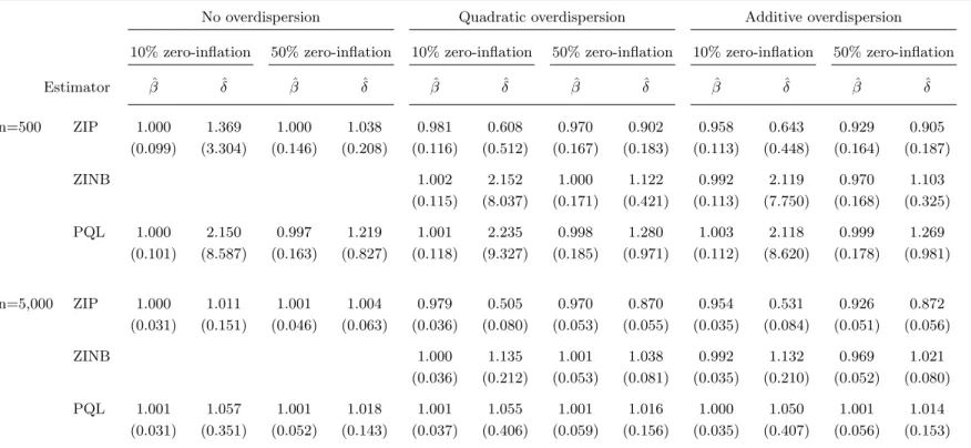
The results of the three simulation setups are displayed in Table 1. The table is divided into three panels, each presenting the results for one of the three setups. Following the focus in the literature, we concentrate on the main parameters of interest, the semi-elasticity of the parent processβ and the change in the log-odds of strategic zerosδ whose true values are 1. The main entries in the tables are the mean of the QL and ML estimates ˆβand ˆδover the 10,000 replications. The numbers in parentheses give the standard deviations.
— Table 1 about here —
The left-hand panel titled “No overdispersion” shows the results for the first setup in which the data generating process is a ZIP model. The first row of results is for the ZIP ML estimator on samples of 500 observations. The ZIP estimates of ˆβ are very close to the true value on average, regardless of whether the degree of zero-inflation is 10% or 50%. Higher degrees of zero-inflation imply less information from which to estimate β, and so the standard deviation is higher with 50% zero-inflation. The opposite is the case withδ. Low degrees of zero-inflation imply having to identify the effect of z on strategic zeros with little information. The Monte Carlo results suggest that 10% zero-inflation may be too little to estimateδreliably with 500 observations: Not only is the standard deviation of ZIP large (3.304), but also the finite sample bias considerable (36.9%). With 50% zero-inflation, the bias is down to 3.8% and the standard deviation to 0.208. PQL estimates β well, too. In the process with 10% zero-inflation, the efficiency loss of PQL is negligible. With 50% zero-inflation it is around 10%. However, the sample size is too small for PQL to estimate δ acceptably. With 5,000 observations, the performance of PQL improves
substiantially. While for β the picture is the same as with the smaller sample, PQL now also obtains satisfactory estimates of δ. However, some finite sample bias is still visible and the efficiency loss relative to ZIP is quite large.
The middle panel (“Quadratic overdispersion”) contains results obtained under the second setup where unobserved heterogeneity is causing the parent model to exhibit quadratic overdis-persion. As ZINB correctly specifies the CEF and the variance function, the panel additionally includes results from this estimator. The pattern for the ZINB ML estimates on 500-observations samples echoes the one for ZIP ML before: Whileβ is estimated quite precisely and free of bias, there is not enough information to get tolerable estimates ofδ. Increasing the sample size to 5,000 improves ZINB’s performance. With 10% and 50% zero-inflation, the remaining biases in δ are 13.5% and 3.8%, respectively. PQL’s performance is quite remarkable here, as its estimates dis-play visibly smaller biases (5.5% and 1.6%). However, its standard deviations are about twice as large as ZINB’s. Regarding the estimation ofβ, there are no noteworthy differences between ZINB and PQL. Inconsistency of ZIP is reflected in substantial biases in all reported mean estimates.
In the right-hand panel, the data are drawn from a process with additive overdispersion ofy∗
, so that both ZIP and ZINB only specify the CEF correctly. ZIP estimation again yields estimators that are not consistent for the true value ofβ in any of the entries of the table. While the biases are not very large, their persistency in the larger sample size unmasks them as asymptotic biases. The biases in the estimated δ, on the other hand, are not only persistent but also very large. The ZINB estimator does not work well either. With 10% zero-inflation and 5,000 observations its performance is similar to before displaying a substiantial bias forδ (13.2%), although now in addition a smaller bias of around -1% is detectable forβ. In the data with 50% zero-inflation the bias inδ is smaller, but the meanβ misses the true value by -3.1%.3 By contrast, the performance
of PQL is much better throughout. Indeed, a look at PQL’s results across the three panels shows that the presence and form of overdispersion bears no effect on its performance.
3
4.3 Further results without exclusion restrictions
In the simulations of Table 1, the regressorsx andz provide independent variation to the parent process and the zero-inflation process, an ideal setting. In applications, regressors are usually correlated. Moreover, exclusion restrictions may often not be justifiable. To address these issues, we repeated the simulations drawing x and z from a bivariate normal distribution with 50% correlation. It is reassuring that results were very similar to those in Table 1. In a next step, we increased the correlation to 100%. This is equivalent to a specification with one regressor which enters both parts of the model. The estimation of such a model demands considerably more of the data, and sample sizes of 500 observations proved too small to get satisfactory results even for the estimation of β. Therefore, Table 2 presents simulation results for the specification without exclusion restrictions with samples of 5,000 and 50,000 observations.
Even with 5,000 observations estimation can be challenging. Correctly specified ZIP ML estimation of the ZIP model is adequate (left-hand panel “No overdispersion”). Likewise, ZINB ML estimation of the quadratic overdispersion process (middle panel) is tolerable, although -reminiscent of the results in Table 1 - estimation of δ with 10% zero-inflation is coupled with substantial finite sample bias. The PQL estimator does not perform well here, suffering from even larger biases. The standard deviation of PQL estimates is about one order of magnitude larger than those of the ML estimates. As we will illustrate with the application in the next section, however, PQL estimation with such sample sizes may not be problematic if additional regressors are available: Variation from more regressors can help estimating the parameters more precisely.
When passing to the results corresponding to 50,000 observations the improvement in PQL’s performance is noteworthy. In all three setups the finite sample bias is only between 0.9%-1.7% forβ and 2.3%-4.5% forδ. While ZIP ML estimation is more precise and less biased in the ZIP setup, it displays large biases of up to -15.4% forβand -82.9% for δin the additive overdispersion setup. In the quadratic overdispersion process, the biases of PQL are often smaller than those of the correctly specified ZINB. Moreover, in the additive overdispersion setup, where ZINB has a similar inconsistency problem as ZIP, it exhibits biases up to -11.6% inβ and 31.2% inδ.
To summarize, the results from the Monte Carlo experiments in this section demonstrate the robustness of the PQL estimator in zero-inflated, finite samples, and the biases that can arise when using its two most common ML competitors.
5
Illustration: demand for physician services
We illustrate PQL estimation of a count model with logit zero-inflation in a well-known health economics application. In particular, the goal is to estimate how health insurance and other socio-demographic characteristics affect the frequency of doctor visits. The dataset is identical to the one used in Cameron and Trivedi (1986). The sample of 5,190 individuals is extracted from the Australian Health Survey 1977-78. The dependent variable is the number of consultations with a doctor or specialist in the two-week period prior to the interview. The mean is 0.302, the variance 0.637. Further details, and a motivation of the selection of explanatory variables, are given in Cameron and Trivedi (1986) and the references quoted therein.
Regressors include demographics (sex, age, age squared), income, various measures of health status (number of reduced activity days (actdays); general health questionnaire score (hscore); recent illness; two types of chronic conditions (chcond1, chcond2)), and three types of health in-surance coverage (levyplus, freepoor, freerepat - the former representing a higher level of coverage and the latter two a basic level supplied free of charge).
Table 3 contains the regression results for the PQL estimator (in the first two columns) as well as for the fully parametric ZIP (in columns 3 and 4) and ZINB (in columns 5 and 6) models. In each case, the same regressors enter the logit model for zero-inflation and the log-linear CEF of the parent model. As discussed earlier, this means that the PQL estimator has two solutions. Since all three estimates of the ZI parameter vectorδ largely coincide in the signs of their elements, it is unlikely that we are erroneously reporting PQL estimates of −δ for the ZI part (and of β+δ for the parent process). Moreover, there is no significant difference in the magnitude of standard errors across models - ZIP’s standard errors are smaller than ZINB’s and PQL’s, the latter two being roughly similar. Thus, the precision of PQL estimation should be fine even though there are no exclusion restrictions.
A likelihood ratio test between ZIP and ZINB clearly favors the latter. While this is an indication of the presence of unobserved heterogeneity and overdispersion, it does not mean, however, that the ZINB is the “right” model. If the overdispersion is misspecified, the ZINB estimator is inconsistent, regardless of fitting the data better than ZIP.
— Table 3 about here —
It is reassuring, therefore, that the parameter estimates are quite insensitive to the choice of specification in many instances, but there are exceptions. For instance, the ZINB model detects no statistically significant effect of having a chronic health condition in either part of the model. Under PQL, the second indicator has large negative and statistically significant effect on the probability of an extra zero and thus increases the expected number of visits. Inferences from PQL and ZINB also differ regarding insurance status. “Freepoor” and “Levyplus” are statistically significant in the ZINB but not so in the PQL model, suggesting some caution in interpreting these effects.
6
Concluding remarks
The main quantities of interest in most count data applications are the conditional expectation function, changes in the probability of strategic zeros, and semi-elasticities of the parent count model with respect to some regressors. For instance, all applications cited in the introduction without exception limited the discussion of their estimation results to the CEF and such effects. This paper proposed a new approach based on Poisson Quasi-Likelihood estimation as a way to estimate these quantities without having to specify more than the CEF, as opposed to the full distribution as is necessary with the traditional ZIP and ZINB ML estimators.
The key advantage of using PQL over ZIP and ZINB is its robustness to misspecification. Given the pervasive uncertainty about the data generating processes in practice, using estimators for ZI models seems unwise if concerns about bias from higher order misspecification exist. The relatively mild misspecifications of the DGP presented in the Monte Carlo experiments frequently resulted in noticeable biases, suggesting that PQL may be the better choice for estimating ZI
models compared to ZI ML estimators in the absence of strong a priori information about the DGP. This conclusion will be the more compelling the larger the data set at hand.
References
Aghion, Philippe, Richard Blundell, Rachel Griffith, Peter Howitt and Susanne Prantl (2009), The Effects of Entry on Incumbent Innovation and Productivity,Review of Economics and
Statistics, 91, 20-32.
Albert A. and J.A. Anderson (1984), On the Existence of Maximum Likelihood Estimates in Logistic Regression Models,Biometrika, 71, 1-10.
Bauer, Thomas, Silja G¨ohlmann and Mathias Sinning (2007), Gender Differences in Smoking Behavior,Health Economics, 16, 895-909.
Cameron, A. Colin, and Pravin K. Trivedi (1986), Econometric models based on count data: Comparisons and applications of some estimators and tests,Journal of Applied
Economet-rics, 1, 29-53.
Cameron, A. Colin, and Pravin K. Trivedi (1998), Regression Analysis of Count Data,
Cam-bridge, MA: Cambridge University Press.
Campolieti, Michele (2002), The recurrence of occupational injuries: Estimates from a zero-inflated count model,Applied Economics Letters, 9, 595-600.
Chang, Fwu-Ranq and Pravin K. Trivedi (2003), Economics of Self-Medication: Theory and Evidence,Health Economics, 12, 721-739.
Clark Ken, Simon A. Peters, and Mark Tomlinson (2005), The determinants of lateness: Evidence from British workers,Scottish Journal of Political Economy, 52(2), 282-304.
Gourieroux, Christian, Alain Monfort and Alain Trognon (1984a), Pseudo Maximum Likelihood Methods: Theory,Econometrica, 52, 681-700.
Gourieroux, Christian, Alain Monfort and Alain Trognon (1984b), Pseudo Maximum Likelihood Methods: Application to Poisson models,Econometrica, 52, 701-721.
Hall, Daniel B., and Jing Shen (2010), Robust estimation for zero-inflated Poisson regression,
Scandinavian Journal of Statistics, 37, 237-252.
Heitmueller, Axel (2004), Job mobility in Britain: Are the Scots different? Evidence from the BHPS,Scottish Journal of Political Economy, 51(3), 329-358.
Ho, Woon-Yee, Peiming Wang and Joseph D. Alba (2009), Merger and acquisition FDI, relative wealth and relative access to bank credit: Evidence from a bivariate zero-inflated count model,International Review of Economics and Finance, 18, 26-30.
Kahn, Matthew E. (2005), The Death Toll from Natural Disasters: The Role of Geography, Income, and Institutions,Review of Economics and Statistics, 87, 271-284.
Keller, Wolfgang, and Arik Levinson (2002), Pollution Abatement Costs and Foreign Direct Investment Inflows to U.S. States,Review of Economics and Statistics, 84, 691-703.
Lambert, Diane (1992), Zero-inflated Poisson regression with an application to defects in man-ufacturing,Technometrics34, 1-14.
List, John A. (2001), Determinants of securing academic interviews after tenure denial: evidence from a zero-inflated Poisson model,Applied Economics, 33, 1423-1431.
Mullahy, John (1986), Specification and Testing of Some Modified Count Data Models,Journal
of Econometrics, 33, 341-365.
Papadopoulos, Georgios, and Joao M.C. Santos Silva (2008), Identification Issues in Models for Underreported Counts, University of Essex, Discussion Paper No. 657.
Pizer, Steven D., and Julia C. Prentice (2011), Time Is Money: Outpatient Waiting Times and Health Insurance Choices of Elderly Veterans in the United States, Journal of Health
Economics, 30, 626-636.
Sari, Nazmi (2009), Physical Inactivity and its Impact on Healthcare Utilization, Health
Sarma, Sisira, and Wayne Simpson (2006), A mircroeconometric analysis of Canadian health care utilization,Health Economics, 15, 219-239.
Sheu, Mei-Ling, Teh-Wei Hu, Theodore E. Keeler, Michael Ong and Hai-Yen Sung (2004), The effect of major cigarette price change on smoking behavior in California: a zero-inflated negative binomial model,Health Economics, 13, 721-791.
Stephan, Paula E., Shiferaw Gurmu, Albert J. Sumell and Grant Black (2007), Who’s patenting in the university? Evidence from the survey of doctorate recipients,Economics of Innovation
and New Technology, 16(2), 71-99.
Street, Andrew, Andrew Jones and Aya Furuta (1999), Cost sharing and pharmaceutical utili-sation and expenditure in Russia,Journal of Health Economics, 18, 459-472.
White, Halbert (1982), Maximum Likelihood Estimation of Misspecified Models,Econometrica,
50, 1-25.
Winkelmann, Rainer (2008),Econometric Analysis of Count Data, fifth edition, Berlin: Springer.
Yen, Stephen T., Chao-Hsiun Tang and Shew-Jiuan B. Su (2001), Demand for Traditional Medicine in Taiwan: A Mixed Gaussian-Poisson Model Approach, Health Economics, 10,
Appendix: Stata code for PQL estimation of zero-inflated count
models
The Stata code below first loads the program for PQL estimation of zero-inflated count models,
pqlzi, and then exemplifies its use with a dataset from the Stata website, fish.dta. The only purpose of the example is to illustratepqlzi’s use; the particular model estimated on this data is nonsensical.
Programpqlziuses mean functionπλinstead of (1−π)λ. We often found this to have better convergence properties. It means that all the estimates from the binary part (eq2-output) have the “wrong” sign. E.g. “-1.81” should be read as “1.81”. If preferred, this can be changed by deleting the two “+ ‘theta2’” bits in the program.
clear all
** Load pqlzi program capture program drop pqlzi program define pqlzi args lnf theta1 theta2 quietly replace ‘lnf’ = ///
- exp(‘theta1’ + ‘theta2’)/(1+exp(‘theta2’)) ///
+ $ML_y1*ln(exp(‘theta1’ + ‘theta2’)/(1+exp(‘theta2’))) /// - lnfactorial($ML_y1)
end
** Use Stata’s example dataset webuse fish
** Get initial values for pqlzi
poisson count persons livebait /* get initial values for count part */ mat po = e(b)
logit count child camper /* get initial values for binary part */ mat lo = e(b)
** Estimate pqlzi model
ml model lf pqlzi (eq1: count = persons livebait) (eq2: child camper), vce(robust) ml init po lo, copy skip /* load initial values */
ml maximize /* estimate pqlzi model */ ** Compare to other ZI models
zinb count persons livebait, inflate(child camper) /* compare to zinb */ zip count persons livebait, inflate(child camper) /* compare to zip */
Table 1: Monte Carlo results
No overdispersion Quadratic overdispersion Additive overdispersion 10% zero-inflation 50% zero-inflation 10% zero-inflation 50% zero-inflation 10% zero-inflation 50% zero-inflation
Estimator βˆ δˆ βˆ δˆ βˆ δˆ βˆ δˆ βˆ δˆ βˆ δˆ n=500 ZIP 1.000 1.369 1.000 1.038 0.981 0.608 0.970 0.902 0.958 0.643 0.929 0.905 (0.099) (3.304) (0.146) (0.208) (0.116) (0.512) (0.167) (0.183) (0.113) (0.448) (0.164) (0.187) ZINB 1.002 2.152 1.000 1.122 0.992 2.119 0.970 1.103 (0.115) (8.037) (0.171) (0.421) (0.113) (7.750) (0.168) (0.325) PQL 1.000 2.150 0.997 1.219 1.001 2.235 0.998 1.280 1.003 2.118 0.999 1.269 (0.101) (8.587) (0.163) (0.827) (0.118) (9.327) (0.185) (0.971) (0.112) (8.620) (0.178) (0.981) n=5,000 ZIP 1.000 1.011 1.001 1.004 0.979 0.505 0.970 0.870 0.954 0.531 0.926 0.872 (0.031) (0.151) (0.046) (0.063) (0.036) (0.080) (0.053) (0.055) (0.035) (0.084) (0.051) (0.056) ZINB 1.000 1.135 1.001 1.038 0.992 1.132 0.969 1.021 (0.036) (0.212) (0.053) (0.081) (0.035) (0.210) (0.052) (0.080) PQL 1.001 1.057 1.001 1.018 1.001 1.055 1.001 1.016 1.000 1.050 1.001 1.014 (0.031) (0.351) (0.052) (0.143) (0.037) (0.406) (0.059) (0.156) (0.035) (0.407) (0.056) (0.153)
Notes: Entries are the average estimates over 10,000 replications. Standard deviations in parenthesis. True value: β=δ= 1.
Table 2: Further Monte Carlo results: No exclusion restriction on regressors
No overdispersion Quadratic overdispersion Additive overdispersion 10% zero-inflation 50% zero-inflation 10% zero-inflation 50% zero-inflation 10% zero-inflation 50% zero-inflation
Estimator βˆ δˆ βˆ δˆ βˆ δˆ βˆ δˆ βˆ δˆ βˆ δˆ n=5,000 ZIP 0.999 1.011 1.000 1.003 0.988 0.488 0.985 0.853 0.865 0.176 0.847 0.673 (0.035) (0.143) (0.063) (0.080) (0.048) (0.105) (0.073) (0.076) (0.063) (0.119) (0.081) (0.076) ZINB 0.983 1.127 0.988 1.030 0.928 1.318 0.880 0.939 (0.044) (0.210) (0.072) (0.100) (0.049) (0.429) (0.081) (0.134) PQL 1.138 1.699 1.136 1.345 1.179 1.896 1.150 1.415 1.180 1.662 1.193 1.423 (0.585) (3.939) (0.713) (1.580) (0.659) (4.499) (0.772) (1.615) (0.658) (3.629) (1.081) (1.870) n=50,000 ZIP 1.000 1.002 1.000 0.999 0.990 0.483 0.984 0.849 0.866 0.171 0.846 0.669 (0.075) (0.043) (0.020) (0.025) (0.014) (0.033) (0.022) (0.023) (0.020) (0.038) (0.024) (0.023) ZINB 0.985 1.107 0.989 1.024 0.930 1.312 0.884 0.925 (0.013) (0.061) (0.022) (0.032) (0.015) (0.120) (0.024) (0.042) PQL 1.011 1.037 1.010 1.023 1.013 1.045 1.009 1.027 1.012 1.038 1.017 1.026 (0.075) (0.211) (0.197) (0.056) (0.084) (0.237) (0.213) (0.065) (0.077) (0.217) (0.211) (0.061)
Notes: Entries are average estimates over 10,000 replications (1,000 repl. for n=50,000). Standard deviations in parenthesis. True value: β=δ= 1.
Table 3: Zero-Inflation models for number of doctor consultations (n=5,190)
PQL ZIP ZINB
Variable ZI Parent ZI Parent ZI Parent
Sex -0.275 0.003 -0.488*** -0.027 -0.592*** 0.010 (0.228) (0.135) (0.171) (0.072) (0.228) (0.084) Age×10−2 8.864** 3.784* 10.496*** 3.128** 10.677** 2.103 (3.986) (2.212) (3.271) (1.297) (4.386) (1.541) Age squared×10−4 -10.611* -3.882* -13.337*** -3.409** -13.821*** -2.187 (4.379) (2.341) (3.690) (1.374) (5.002) (1.639) Income -0.269 -0.288 -0.437* -0.295*** -0.365 -0.214 (0.349) (0.203) (0.264) (0.113) (0.346) (0.133) Levyplus -0.381 -0.032 -0.433** -0.034 -0.640** -0.095 (0.253) (0.158) (0.197) (0.096) (0.264) (0.114) Freepoor 0.278 -0.385 0.308 -0.377 0.111 -0.481* (0.830) (0.512) (0.508) (0.239) (0.659) (0.283) Freerepat -0.974** -0.254 -1.149*** -0.215* -1.375*** -0.189 (0.339) (0.202) (0.305) (0.117) (0.447) (0.140) Illness -0.345** 0.002 -0.416*** 0.049** -0.672*** 0.052* (0.092) (0.045) (0.081) (0.025) (0.156) (0.029) Actdays -1.114** 0.047*** -1.256*** 0.083*** -1.787*** 0.104*** (0.198) (0.014) (0.238) (0.006) (0.653) (0.008) Hscore -0.080* 0.016 -0.097** 0.018 -0.105* 0.023* (0.043) (0.020) (0.039) (0.011) (0.056) (0.014) Chcond1 -0.242 -0.078 -0.127 -0.013 -0.119 -0.000 (0.262) (0.164) (0.199) (0.092) (0.279) (0.108) Chcond2 -0.754** -0.144 -0.604** -0.034 -0.489 0.055 (0.352) (0.180) (0.306) (0.103) (0.414) (0.121) Const. 1.452** -0.618 0.786 -1.050*** 0.622 -1.233*** (0.739) (0.472) (0.572) (0.255) (0.753) (0.296) α 0.578 (.086) Log-likelihood -3,174.2 -3,107.6
Notes: Standard errors in parentheses (robust standard errors for PQL). ***, **, * denote statistical significance at the 1%, 5%, 10% significance levels, respectively. αindicates the overdispersion parameter of the negative binomial type II distribution.
Working Papers of the Socioeconomic Institute at the University of Zurich
The Working Papers of the Socioeconomic Institute can be downloaded from http://www.soi.uzh.ch/research/wp_en.html
0908
Consistent estimation of zero-inflated count models, Kevin E. Staub, Rainer
Winkelmann, Revised version, August 2011, 21 p.
0907
Competitive Screening in Insurance Markets with Endogenous Wealth
Heterogeneity, Nick Netzer, Florian Scheuer, April 2009, 28 p.
0906
New Flight Regimes and Exposure to Aircraft Noise: Identifying Housing Price Effects
Using a Ratio-of-Ratios Approach, Stefan Boes, Stephan Nüesch, April 2009, 40 p.
0905
Patents versus Subsidies – A Laboratory Experiment, Donja Darai, Jens Großer,
Nadja Trhal, March 2009, 59 p.
0904
Simple tests for exogeneity of a binary explanatory variable in count data regression
models, Kevin E. Staub, February 2009, 30 p.
0903
Spurious correlation in estimation of the health production function: A note, Sule
Akkoyunlu, Frank R. Lichtenberg, Boriss Siliverstovs, Peter Zweifel, February 2009,
13 p.
0902
Making Sense of Non-Binding Retail-Price Recommendations, Stefan Bühler, Dennis
L. Gärtner, February 2009, 30 p.
0901
Flat-of-the-Curve Medicine – A New Perspective on the Production of Health,
Johnnes Schoder, Peter Zweifel, January 2009, 35 p.
0816
Relative status and satisfaction, Stefan Boes, Kevin E. Staub, Rainer Winkelmann,
December 2008, 11 p.
0815
Delay and Deservingness after Winning the Lottery, Andrew J. Oswald, Rainer
Winkelmann, December 2008, 29 p.
0814
Competitive Markets without Commitment, Nick Netzer, Florian Scheuer, November
2008, 65 p.
0813
Scope of Electricity Efficiency Improvement in Switzerland until 2035, Boris Krey,
October 2008, 25 p.
0812
Efficient Electricity Portfolios for the United States and Switzerland: An Investor
View, Boris Krey, Peter Zweifel, October 2008, 26 p.
0811
A welfare analysis of “junk” information and spam filters; Josef Falkinger, October
2008, 33 p.
0810
Why does the amount of income redistribution differ between United States and
Europe? The Janus face of Switzerland; Sule Akkoyunlu, Ilja Neustadt, Peter Zweifel,
September 2008, 32 p.
0809
Promoting Renewable Electricity Generation in Imperfect Markets: Price vs. Quantity
Policies; Reinhard Madlener, Weiyu Gao, Ilja Neustadt, Peter Zweifel, July 2008,
34p.
0808
Is there a U-shaped Relation between Competition and Investment? Dario Sacco,
July 2008, 26p.
0807
Competition and Innovation: An Experimental Investigation, May 2008, 20 p.
0806
All-Pay Auctions with Negative Prize Externalities: Theory and Experimental
Evidence, May 2008, 31 p.
0805
Between Agora and Shopping Mall, Josef Falkinger, May 2008, 31 p.
0804
Provision of Public Goods in a Federalist Country: Tiebout Competition, Fiscal
Equalization, and Incentives for Efficiency in Switzerland, Philippe Widmer, Peter
Zweifel, April 2008, 22 p.
0802
The effect of trade openness on optimal government size under endogenous firm
entry, Sandra Hanslin, March 2008, 31 p.
0801
Managed Care Konzepte und Lösungsansätze – Ein internationaler Vergleich aus
schweizerischer Sicht, Johannes Schoder, Peter Zweifel, February 2008, 23 p.
0719
Why Bayes Rules: A Note on Bayesian vs. Classical Inference in Regime Switching
Models, Dennis Gärtner, December 2007, 8 p.
0718
Monoplistic Screening under Learning by Doing, Dennis Gärtner, December 2007,
29 p.
0717
An analysis of the Swiss vote on the use of genetically modified crops, Felix
Schläpfer, November 2007, 23 p.
0716
The relation between competition and innovation – Why is it such a mess? Armin
Schmutzler, November 2007, 26 p.
0715
Contingent Valuation: A New Perspective, Felix Schläpfer, November 2007, 32 p.
0714
Competition and Innovation: An Experimental Investigation, Dario Sacco, October
2007, 36p.
0713
Hedonic Adaptation to Living Standards and the Hidden Cost of Parental Income,
Stefan Boes, Kevin Staub, Rainer Winkelmann, October 2007, 18p.
0712
Competitive Politics, Simplified Heuristics, and Preferences for Public Goods,
Felix Schläpfer, Marcel Schmitt, Anna Roschewitz, September 2007, 40p.
0711
Self-Reinforcing Market Dominance,
Daniel Halbheer, Ernst Fehr, Lorenz Goette, Armin Schmutzler, August 2007, 34p.
0710
The Role of Landscape Amenities in Regional Development: A Survey of Migration,
Regional Economic and Hedonic Pricing Studies,
Fabian Waltert, Felix Schläpfer, August 2007, 34p.
0709
Nonparametric Analysis of Treatment Effects in Ordered Response Models,
Stefan Boes, July 2007, 42p.
0708
Rationality on the Rise: Why Relative Risk Aversion Increases with Stake Size,
Helga Fehr-Duda, Adrian Bruhin, Thomas F. Epper, Renate Schubert, July 2007,
30p.
0707
I’m not fat, just too short for my weight – Family Child Care and Obesity in
Germany, Philippe Mahler, May 2007, 27p.
0706
Does Globalization Create Superstars?,
Hans Gersbach, Armin Schmutzler, April 2007, 23p.
0705
Risk and Rationality: Uncovering Heterogeneity in Probability Distortion,
Adrian Bruhin, Helga Fehr-Duda, and Thomas F. Epper, July 2007, 29p.
0704
Count Data Models with Unobserved Heterogeneity: An Empirical Likelihood
Approach, Stefan Boes, March 2007, 26p.
0703
Risk and Rationality: The Effect of Incidental Mood on Probability Weighting,
Helga Fehr, Thomas Epper, Adrian Bruhin, Renate Schubert, February 2007, 27p.
0702
Happiness Functions with Preference Interdependence and Heterogeneity: The Case
of Altruism within the Family, Adrian Bruhin, Rainer Winkelmann, February 2007,
20p.
0701
On the Geographic and Cultural Determinants of Bankruptcy,
Stefan Buehler, Christian Kaiser, Franz Jaeger, June 2007, 35p.
0610
A Product-Market Theory of Industry-Specific Training,
Hans Gersbach, Armin Schmutzler , November 2006, 28p.
0609
Entry in liberalized railway markets: The German experience,
Rafael Lalive, Armin Schmutzler, April 2007, 20p.
0608
The Effects of Competition in Investment Games,