A Balanced Secondary Structure Predictor

(1)

University of New Orleans University of New Orleans

ScholarWorks@UNO

University of New Orleans Theses and

Dissertations Dissertations and Theses

Spring 5-15-2015

A Balanced Secondary Structure Predictor

Md Nasrul Islam

University of New Orleans, [email protected]

Follow this and additional works at: https://scholarworks.uno.edu/td Part of the Other Computer Engineering Commons

Recommended Citation Recommended Citation

Islam, Md Nasrul, "A Balanced Secondary Structure Predictor" (2015). University of New Orleans Theses and Dissertations. 1995.

https://scholarworks.uno.edu/td/1995

This Thesis is protected by copyright and/or related rights. It has been brought to you by ScholarWorks@UNO with permission from the rights-holder(s). You are free to use this Thesis in any way that is permitted by the copyright and related rights legislation that applies to your use. For other uses you need to obtain permission from the rights-holder(s) directly, unless additional rights are indicated by a Creative Commons license in the record and/or on the work itself.

(2)

A Balanced Secondary Structure Predictor

A Thesis

Submitted to the Graduate Faculty of the University of New Orleans In partial fulfillment of the Requirements for the degree of

Master of Science in

Computer Science

by

Md Nasrul Islam

(3)

ii

Acknowledgement

First of all, I would like to humbly express my profound gratitude to my supervisor Dr. Md Tamjidul Hoque for being so kind, enduring and at the same time vigilant in every aspect of my

research and academic progress during the whole time I have been here at University of New Orleans. He has been tireless to explain every nuances again and again till I felt little uncomfortable

to understand any concept. I must appreciate his continuous guidance, critical and insightful advice, helpful and inspiring criticism, valuable suggestions and commendable support and quick feedbacks to my queries throughout the way towards completion of my thesis.

Secondly, I would like thank Dr. Christopher M. Summa and Dr. N. Adlai A. DePano for their kind consent to be a board member of my thesis committee, despite their hectic schedule and

important other priorities.

I would also like to thank University of New Orleans for providing me an excellent environment for research and financial support in the form of graduate research assistantship.

I must mention my adorable wife and also my lab partner, Sumaiya Iqbal, for her continuous encouragement and support, each and every day in every aspect of my life. And I would

(4)

iii

List of Figures

Figure 1: (a) An amino acid with its bonds, (b) An amino acid at pH 7.0. ... 8

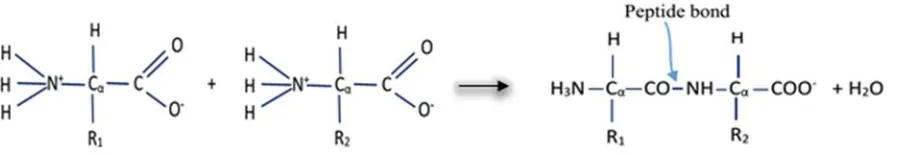
Figure 2: Condensation reaction that forms protein chain by developing peptide bond between two amino acids. Here R1 and R2 stand for side chains. ... 9

Figure 3: Tertiary structure of protein with secondary structure component [39]. ... 13

Figure 4: Tertiary structure of protein. This is a cartoon image of a protein (PDB ID: 1AV5) generated by Jmol, an open source Java based viewer for chemical structures. ... 15

Figure 5: A simple example of protein quaternary structure is the structure of Quinone reductase. This is a cartoon image collected from PDB (PDB ID: 1QRD) generated by Jmol, an open source Java based viewer for chemical structures. ... 16

Figure 6: Yearly growth of X-ray crystallographic structure. Source: PDB [36, 37] ... 19

Figure 7: Yearly growth of NMR structure. Source: PDB [36]. ... 24

Figure 8: A hidden Markov model with 3 hidden states– s1, s2, ands3 and m number of observations denoted by oi that may be emitted from any of these states. Here, 1 ≤ i ≤ m. We also see a start state here. This start state is actually a pseudo state which emits no symbol, rather just indicates the start of the sequence. Here the arrows from one state to another or to itself represent the transitions from one state to another or self-transition, whereas the arrows from states to symbols represent the emission of symbols from corresponding states. ... 33

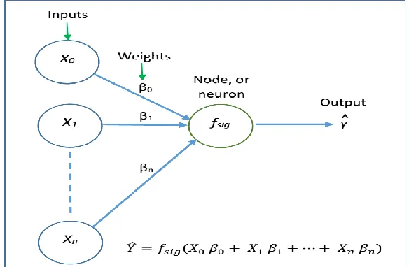
Figure 9: A single neuron or node of an ANN. fsig is the activation function which determines the output. Here xi are the features used, where n = number of feature and i = 1, 2, 3, …n. X0 is known as bias term. ... 39

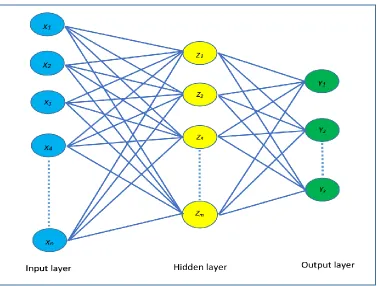
Figure 10: Schematic diagram of a single hidden layer feed-forward neural network with k different output. The units in the middle of the networks are known as hidden nodes. Each node has a derived feature Zm computed form the input of the preceding layer nodes. Here maximum value of m is the number of hidden nodes in a particular hidden layer. ... 40

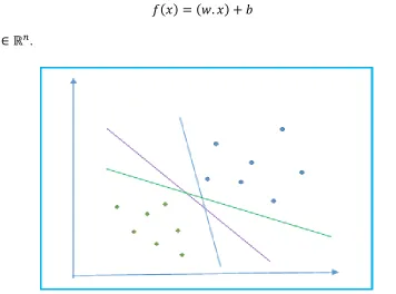
Figure 11: A simplified two class classification problem is shown here. The circular and diamond shaped data points belong to two different classes. The classes may be separated by many different decision boundaries as shown by the solid lines. ... 44

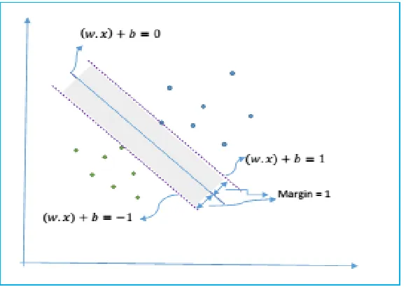
Figure 12: Support vector classifier. The solid line represents the decision boundary while the dashed lines are the boundaries of maximal margin area, shown as shaded area. Data points on the dashed lines are the support vectors. The 1 or -1 values on the right hand side of the equations of the margin boundaries represent the scaled distance from the decision line of the nearest points that belong to +1 and -1 class respectively. ... 45

Figure 13: Algorithm for combining cSVM and SPINE X... 49

Figure 14: This figure demonstrate a cross over operation. C1, and C2 are survival probability based selections as crossover candidates. nC1, and nC2 are two new chromosomes created after crossover. The green highlighted bit in C1 and C2 indicate the randomly selected crossover site. Similar color curly braces show the origin of the part in new chromosome. ... 50

Figure 15: Pseudo code for GA... 51

Figure 16: Binary class accuracies on CB475dataset for different feature set based models. ... 60

Figure 17: Accuracy of E/~E SVM predictor at different window size. ... 61

Figure 18: Comparison of accuracy along with over prediction rate on CB471dataset. ... 63

(7)

vi

(8)

vii

List of Tables

Table 1: A summary of the secondary structure composition of T552test dataset ... 52

Table 2: A summary of the secondary structure composition of CB471test dataset. ... 53

Table 3: A summary of the secondary structure composition of N295test dataset. ... 54

Table 4: A list of all features used in this research. ... 56

Table 5: Description of the feature sets used. ... 57

Table 6: Evaluation criteria. ... 57

Table 7: Comparison of performance of models trained with f29and f51feature sets. ... 58

Table 8: Comparison of the performance of using f29and f51features sets. CB475dataset was extracted from CB513dataset to ensure that the test set is no more than 25%similar to training set to ensure more robust comparison. ... 59

Table 9: Comparison of the performance of using f29and f31features sets. CB475dataset was extracted from CB513dataset to ensure that the test set is no more than 25%similar to training set to ensure more robust comparison. ... 60

Table 10: Accuracy of secondary structure prediction on CB471test dataset. ... 62

Table 11:Precision and recall of secondary structure prediction on CB471test dataset. ... 64

Table 12: Accuracy of secondary structure prediction on N295test dataset. ... 66

Table 13: Precision and recall of secondary structure prediction on N295test dataset. ... 68

Table 14: Rank of all predictors across different performance measure on CB471 test data set. ... 70

(9)

viii

Abstract

Secondary structure (SS) refers to the local spatial organization of the polypeptide backbone atoms

of a protein. Accurate prediction of SS is a vital clue to resolve the 3D structure of protein. SS has three different components- helix (H), beta (E) and coil (C). Most SS predictors are imbalanced as

their accuracy in predicting helix and coil are high, however significantly low in the beta. The objective of this thesis is to develop a balanced SS predictor which achieves good accuracies in all three SS components. We proposed a novel approach to solve this problem by combining a genetic

algorithm (GA) with a support vector machine. We prepared two test datasets (CB471 and N295) to compare the performance of our predictors with SPINE X. Overall accuracy of our predictor

was 76.4% and 77.2% respectively on CB471 and N295 datasets, while SPINE X gave 76.5% overall accuracy on both test datasets.

(10)

1

1. Introduction

1.1 Introduction

In the modern scientific world bioinformatics has attained a very crucial position as a research discipline, promising the potential of benefitting human endeavor to understand and analyze

biological phenomena. It is a multidisciplinary field where computer scientists can provide biologists critical tools to study genomics, proteomics, medicine and many more. Proteomics, as a discipline, studies the function and structure of proteins and requires the processing and analysis

of enormous amounts of data. The number of different structures and functions of proteins in a single organism is staggering [1]. Considering either from a quantitative or a functional

perspective, proteins are arguably the most important macromolecules in all living organisms. They make possible all of the chemical reactions in living cells [1]. More than half of the dry weight of cells are constituted by proteins of various shapes and sizes and they play a significant

role in the functions of cells. Chemical organization of proteins is relatively simple. They are linear chains of amino acids connected through covalent bonds commonly known as peptide bonds [2].

The main constituents of proteins, amino acids, are small molecules with a common backbone consisting of several C, H, O, and N atoms and a side chain with up to 30 more atoms. This apparently simple linear chain of amino acids adopts a specific folded three-dimensional (3D)

shape, which enables proteins to perform various tasks. This 3D shape of a particular protein may not remain fixed, rather, the protein may explore a wide array of kinetically accessible conformations. The spatial arrangement of atoms in a protein macromolecule is called its

(11)

2

are not equally probable. The conformation that exists under a given set of conditions is usually the one that is thermodynamically most stable and has the lowest Gibbs free energy. This structural

dynamism also yields additional functionality to proteins. Some examples of tasks carried out by proteins are transportation of small molecules such as haemoglobin that transports oxygen in the

bloodstream, storage, as done by ferritin for iron storage and release, catalyzing biological functions, providing structure to collagen and skin, controlling sense, regulating hormones, processing emotion, etc. [3]. Without the catalyzing effect of proteins, many chemical reactions in

the cell of living organism would happen in a rate which can be deemed as negligible [1]. Knowledge about the structure of a protein reveals important information about the location of

probable functional or interaction sites, distantly related protein identification, and detection of the important regions of the protein sequence which are crucial in maintaining the structure of the protein, and so on [4]. A widely accepted fundamental principle in protein science is that protein

structure leads to protein function [5]. For these reasons, prediction of protein structure and function has become one of the most important problems in molecular biology. The first successful

discovery of protein structure is credited to Max Perutz and John Kendrew of Cambridge University [6]. Perutz and John Kendrew discovered the high resolution structure of myoglobin and hemoglobin respectively through X-ray crystallography. Since then, X-ray crystallography has

been the most widely used experimental method to determine protein structure. Over 80% of the three-dimensional macromolecular structure data in the Protein Data Bank (PDB) were obtained

by X-ray crystallography [7]. Nuclear magnetic resonance (NMR) spectroscopy is the second most widely used experimental method for obtaining three dimensional structure of proteins at atomic level resolution [8]. More than 10,000 structures, about 16% of the total structures in PDB, have

(12)

3

very time consuming as well as expensive. For example, one experiment cost around $250,000 in 2000 and $65,000 in 2008 [9]. One structure determination through such experimental methods

may take months or even years [10]. The drawbacks of experimental methods are not limited to time and cost only. For some proteins it is not possible to apply such experimental methods. For

example, X-ray crystallography is extraordinarily difficult for membrane protein structure determination. Protein molecules with highly hydrophobic portions generally cannot be crystallized [11]. NMR techniques cannot be applied for larger proteins of size more than 100

KDa. On the other hand, computational approaches have the potential to overcome the previously mentioned difficulties or disadvantages associated with the experimental approaches by utilizing

the correlation between the primary sequence information and the final 3D structure. During the last several decades the amount of biological data has rapidly increased. Genome sequences of a number of species, including human, have been completely mapped thanks to the world-wide

genome sequencing project. The gap between the number of known sequence and the number of known structures is widening rapidly [12]. A detailed understanding of the biological role of the

majority of proteins is not possible through genome sequencing alone, rather we need structural and functional information for that [13]. With increasing research to discover new biological processes and to master existing known processes, the development of well performing and new

computational tools becomes increasingly necessary and useful. If the path of protein folding from sequence to 3D structure can be properly modeled, it will bring about radical benefits in combating

many diseases by solving either fully or partially various currently existing crucial medical, agricultural and biotechnological bottlenecks. Therefore, high throughput computational models for the prediction of protein structure from sequence is an immediate need. For this reason

(13)

4

of genetics [14]. The principle of Anfinsen asserts that all information required to specify the structure of a protein is encoded in its amino acid sequence [15, 16]. However this task of

predicting the 3D structure of protein from sequence information is not straight forward as how to read this information off of the sequence so as to reconstruct 3D structure remains unclear [17].

Mostly because proteins exhibit some general patterns and a degree of regularity in their folding, it is possible to apply computational techniques to investigate this challenging problem. Although prediction of protein 3D structures is the ultimate target, the structure yet cannot be accurately

predicted directly from sequences [12]. However this final 3D structure prediction problem is usually approached by solving course-grained intermediate problems such as secondary structure

prediction (SSP) [12, 18, 19]. Secondary structure (SS) refers to the local spatial organization of a polypeptide backbone atoms of a protein [20]. It may be deemed as a notion of residue-level local sub-structure. Secondary structures are determined by examining the pattern of hydrogen bonds

between side chains and amino acid residues in a protein. As proposed by Pauling and his colleagues, there are mainly two types of secondary structure- alpha helix (α) or helix (H) and beta (β) strand or beta sheet (E) [21]. These are all regular polypeptide folding patterns. Dominant

hydrogen bonding patterns are turn and bridge. Repeated turns give rise to helixes while repeated bridges generate strands [22]. However another type, turn or coil (C), is also considered as a kind

of secondary structure. The third type is generally referred to the structure of those residues which are neither helix nor beta sheet. Prediction of SS greatly simplifies the ultimate 3D structure

prediction problem [12].

From a machine learning point of view, SSP is a classification problem, where based on relevant features we have to decide on each amino acid in a protein belongs to protein secondary

(14)

5

SSP problem has been approached using various machine learning algorithms including neural networks (NN), hidden Markov model (HMM), support vector machine (SVM), etc. Such machine

learning approaches used so far for SSP vary in basic algorithm used, and/or in feature sets employed. Despite numerous effort the accuracy of SSP stuck at around 80% for last five decades.

This accuracy is also very much dataset dependent. Needless to say, the increase in accuracy of

SSP, is crucial for biological and medical development.

In this thesis, we have employed SVM with a radial basis function (RBF) kernel, along with several novel features such as disorder probability, bigram and monogram. SVM is a well performing algorithm in biological application compared with other machine learning algorithms

as they are effective in controlling the classifier’s capacity and the associated potential for over fitting ensuring maximum margin of the decision boundary separating two classes [18]. Instead

of directly trying three class classification, we have employed three binary classifiers viz- H/~H, E/~E and C/~C separately and then to combine. This provides us the opportunity to efficiently attack the problem in simpler form and then to optimally combine them. We consolidated the

predictions from these three binary classifiers to come up with a final three class prediction with optimal weighting using heuristics obtained from a genetic algorithm. We also developed a

meta-predictor by combining the prediction of our combined SVM meta-predictor and SPINE X [23], a state-of-the-art secondary structure predictor. Our meta-predictor comes up with a highly balanced overall prediction as well as the prediction of three secondary structure components with higher

accuracy and improving the accuracy of beta structure prediction significantly in particular.

1.2 Motivation

Since the 3D structure of protein is a pivotal clue to the study of a protein’s function, a good

(15)

6

predict protein 3D structure. Despite numerous experimental and analytical endeavors, protein 3D structure prediction is still an unresolved problem. This issue is commonly known as the protein

folding problem. Notable pioneers, Pauling and Corey devoted decades to find way to predict the accurate structure of amino acids, peptides and other substances that construct the structure of

protein. They suggested that interatomic distances, bond angles and other configurational parameters might aid such prediction [21]. They used such information to develop models of two different hydrogen bonded helical conformations, keeping in mind that such things are likely to

develop significant part of the structure of both globular and fibrous proteins. With thorough analysis of different bond length, hydrogen bond distances and neighboring atoms’ influences,

they proposed the idea of helices with different non-integer number of residues per helix. They also proposed the idea of a planar peptide bond that drastically simplifies the study and the understanding of protein structure. This successful prediction of alpha helix is a significant

contribution of Linus Pauling. He achieved it due to his assumptions of planar peptide bonds, equivalency of amino acids with respect to backbone conformation and hydrogen bonds between

amide protein and the O atom of adjacent residue with an N–O bond distance of 2.72 Å [24]. In this regard, a significant contribution is Anfinsen’s work [25, 26].

Anfinsen and his colleagues established the “Thermodynamic hypothesis” that the three

dimensional structure of a protein in its native environment is the one that minimizes Gibbs free energy of the whole system. This notion ultimately translates into that the native structure is

determined by inter atomic interaction, hence by the sequence of amino acids of protein. This finding brought Anfinsen Nobel prize in 1972. Guzzo in 1965 suggested significant influence of amino acid sequence on the location of helical and non-helical part of a protein structure based on

(16)

7

emphasized on the notion that without considering other components of the cell, the enzymatically active secondary and tertiary structure of protein may be resolved solely from the interaction

between and amino acids and solvent in a solution. For instance, Guzzo said that presence of proline, aspartic acid, glutamic acid, or histidine are important to form a helical disruption.

Further, the famously known Levinthal Paradox suggests that proteins fold into their specific 3D conformations in a time-span way [28] shorter than it would be possible for protein molecules to actually search the entire conformational space for the lowest energy state. Therefore,

hierarchical approaches are very suitable for this critical problem solving. Secondary structure prediction is a critical building block towards protein fold recognition. One reason is that

secondary structure gives local structural preferences which limits the possible number of configurations to each part of a polypeptide chain. In the amino and carboxyl termini of alpha helices, often very strong sequence-structure correlations are observed [29]. Therefore, secondary

structure information significantly reduces the conformational search space for fold recognition. Accurately computing protein structure is also important for crucial biological applications such

as virtual ligand screening [9, 30], structure based protein function prediction [31] and structure based drug design [32]. Therefore, every single advancement towards solving the protein folding problem is vitally important for human kind. For all these reasons we have taken the challenge to

(17)

8

2. Background and Related Works

2.1 Fundamentals of Protein

Proteins are the most versatile macromolecules in living organisms and play significant roles essentially in all biological processes [33]. Proteins are large biological polymers composed of single or multiple chain of amino acid residues. An amino acid is an organic compound that has a central carbon atom, usually known as alpha carbon (Cα) or chiral carbon that uses its four valences to create bond with a carboxylic group, an amino group, a hydrogen atom and a side chain. A simple amino acid molecule along with its ionic condition is shown in the Figure 1.

Figure 1: (a) An amino acid with its bonds, (b) An amino acid at pH 7.0.

Side chains are unique features of amino acids. Side chains distinguish one amino acid from other

amino acids. Their interaction in protein with the surroundings depends on this side chain. Depending on the nature of this side chain, the properties of different amino acids also vary. They

can be hydrophilic, hydrophobic, acidic or basic, etc. The simplest side chain may be a hydrogen atom (H). In general 20 different amino acids are found in protein molecules. These amino acids are monomeric building block of protein. Protein length is usually expressed in terms of amino

(18)

9

from fewer than 20 to more than 5000, however on an average a protein has 350 amino acid residues. The possible space for variation of protein could be as large as 204500 _{or 10}5850_{[1]. Protein}

structure and function are mainly determined by the sequence of amino acids in a particular polymer. Two adjacent amino acids are connected through linear peptide bond. Peptide bonds, a

type of covalent bond, are created through a condensation reaction between the carboxylic group of one amino acids and the amino group of another adjacent amino acid. The general reaction that forms the peptide bond backbone of proteins is shown in Figure 2 below:

Figure 2: Condensation reaction that forms protein chain by developing peptide bond between two amino acids. Here R1 and R2 stand for side chains.

Compound created through peptide bonds are known as polypeptide. In this sense proteins are also polypeptides, however only short chains of amino acids are usually known as polypeptides. The polypeptide chain begins with the amino group and ends with the carboxyl group. Terminal with

amino groups is also known as N- terminus while the terminal with carboxyl group is known as C- terminus. Every protein has a unique amino acid sequence. This sequence is based on the codons

(19)

10

From chemical point of view, proteins are one of the most complex and functionally important molecules [35]. Important properties that enable proteins for a wide variety of functions [33] are

discussed below:

 Polymer type: Proteins are made up of only 20 different amino acids, the combination of those amino acids greatly varies. Such variation of combining amino acids make possible formation of myriad number of different proteins with

different functionalities.

 Functional groups: Protein molecules may contain a wide variety of functional groups such as alcohols, thiols, thioethers, carboxylic acids, carboxamides, etc. These functional groups are oriented in protein molecules in numerous fashion,

which give rise to a broad spectrum of protein functionality. They also interact in such a way that the chemical reactivity of amino acid side chains enhances [35].  Formation of complex assembles: Proteins are capable of interacting with one

another and with other biological macromolecules. Such interactions enable proteins to form complex assemblies. These assemblies may act as

macro-molecular machines which are capable of precisely replicating DNA, transmitting signals within cells, and also helping in many other essential biological processes.  Mix of structural rigidity and flexibility: Some parts of the protein structure may be

very rigid which may act as the skeleton of the macro-molecule while other parts

may be flexible. These flexible parts with their limited flexibility may work as hinges, springs, and levers and may assist in assembling of proteins with one another and with other molecules into complex units, and in transmitting

(20)

11

 Diversity in size, shape and chemical properties: Protein size varies; as we have noted earlier that the number of amino acid residues in a protein may vary from only 20 to many thousands. Protein may be hydrophobic, hydrophilic, fibrous, globular etc. Proteins may also have affinity to binding to a variety of different

compounds, atoms or molecules commonly known as prosthetic groups [1]. Prosthetic groups may be organic such as vitamin or inorganic such as metal ions

that may bind to a specific site of a protein and are important for different functionality of proteins. All these different features add to the spectrum of diverse functionality of protein. A well-known example of prosthetic group is heme which

binds oxygen to protein hemoglobin.

2.2 Structure of a Protein

A fundamental principle in protein science is that the protein structure leads to protein function

[5]. If we want to know how proteins function, we must know the structure of the proteins accurately. Therefore, the study of protein function is inseparable from the study of protein

structure.

It has been though for a long time that proteins are random colloids of structures until it

was shown by Bernal and Crowfoot that if a crystal of pepsin yields a discrete diffraction pattern if placed in a beam of X-ray [36]. This finding is a pioneering evidence that protein structures are not random colloid rather a large structured molecule consists of ordered array of atoms. Now

through studies on a large number of proteins it has been established that protein shows significant degree of structural regularities in terms of repetitive structural patterns, which may be classified

(21)

12

Following discussion focuses on the levels of structure of protein. Protein structures are usually categorized into the following four levels’ of complexities:

 Primary structure  Secondary structure  Tertiary structure and  Quaternary structure

2.2.1 Primary structure

Primary structure is defined as the linear sequence of amino acids. Sequence of amino acids in a particular protein is not random, rather fixed which was first discovered by Frederick Sanger [37].

He established this idea for protein insulin and for the first time determining the complete amino acid sequence of a protein, the B chain of insulin. B chain is one of the two polypeptide chains that form the insulin. Before this discovery, the predominant notion was that the proteins are random

molecules with a kind of center of gravity as well as with appreciable micro-heterogeneity [38]. Therefore, this work of Sanger brought about paradigm shift in the knowledge of scientists in this

field.

Although proteins are linear sequence of amino acids, detail and specific mapping of its

structure from the sequence is not straightforward, rather it has remained as a widely studied yet to solve critical problem of molecular biology.

2.2.2 Secondary structure

Secondary structure (SS) refers to the local spatial organization of a polypeptide’s backbone atoms

of a protein [20]. Secondary structures are determined by examining the pattern of hydrogen bonds

(22)

13

structure- alpha helix (α) or helix (H) and beta (β) strand or beta sheet (E) [21]. These are all regular polypeptide folding patterns. Dominant hydrogen bonding patterns are turn and bridge.

Repeated turns give rise to helixes while repeated bridges generate strands [22]. However another type, turn or coil (C), is also considered as a kind of secondary structure. The third type is generally

referred to the structure of those residues which are neither helix nor beta sheet. In Figure 3 a protein 3D structure with secondary components is shown. To classify the secondary structure, we investigate the geometric properties of peptides to verify their formations.

Figure 3: Tertiary structure of protein with secondary structure component [39].

However, when the structure or, the geometric properties are not yet discovered, we rely on

prediction from the primary sequences alone. The task of secondary structure prediction basically is to predict to which of these three types of structures (α, β or turn) each residue in a particular

sequence belongs. For example, if we consider

LLATGCLLKNKGKSEHTFTIKKLGIDVVVESG…. – a primary sequence of a protein, a

secondary structure prediction method may suggest, say, from first L to the first K are in helix,

(23)

14

secondary structure prediction does not give the complete 3D structure of a protein, which is the famous folding problem. While complete understanding of protein folding is excruciatingly

complicated, however, the problem is usually tried through simpler steps and secondary structure prediction is one such very prominent step [40]. Predicting secondary structure is also important

because there is a strong coupling between secondary and tertiary structure of proteins [41]. Accurate prediction of SS is urgent, since predicted SS is an essential input feature for other important predictors such as tertiary protein structure predictor, disorder predictor, binding and

non-binding predictor, statistical energy function, etc. Successful SSP can also help us to step forward to answer the reasons behind many critical diseases such as Cancer, Cardiovascular

diseases, Alzheimer's disease, type two diabetes, Parkinson's disease and many more.

2.2.3 Tertiary structure

Tertiary structure refers to the folding of its secondary structure element by specifying the position

of each atom in the protein in a three dimensional structure. Scope of secondary structure is within the spatial arrangement of adjacent amino acid residues. On the other hand, tertiary structure encompasses longer-aspects of amino acid sequence by capturing the interactions of amino acids

in the polypeptide sequence that are far apart and belongs to different types of secondary structures. These distant amino acids with respect to their positions in the primary sequence may come closer

when the protein folds and interacts within the completely folded structure of a protein. Therefore, we might say that while secondary structure is all about local sub-structure patterns, tertiary

structure is defined as the global structural conformation of proteins. Although it is well established that the sequence of amino acids determines the three dimensional structure of proteins, precise mapping of three dimensional structure and amino acid sequence remains a big challenge [1].

(24)

15

within certain geometric constraints. These different three dimensional structures of same protein are known as conformations. This conformational variability, however difficult to capture, is very

important for protein functioning [1, 42, 43].

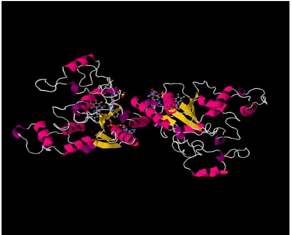
Figure 4: Tertiary structure of protein. This is a cartoon image of a protein (PDB ID: 1AV5) generated by Jmol, an open source Java based viewer for chemical structures.

2.2.4 Quaternary structure

We know that proteins are polypeptide chains. In some instances, two or more polypeptide chains known as subunits may combine and form a structure different from regular tertiary structures,

whereas in contrast the tertiary structure consist of a single polypeptide chain. Spatial arrangement of these subunits is known as protein quaternary structure [20]. The subunits may be identical or

different. The simplest type of quaternary structure consists two identical subunits. This type of structure is known as homo-dimer [44]. An example structure of homo-dimer is shown in Figure 5. In a quaternary structure, there may exist more than 2 subunits as well. Two or more subunits

(25)

16

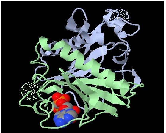
Figure 5: A simple example of protein quaternary structure is the structure of Quinone reductase. This is a cartoon image collected from PDB (PDB ID: 1QRD) generated by Jmol, an open source Java based viewer for chemical structures.

Quaternary structures are sometimes crucial for some important functions. Interactions among subunits in quaternary structure play a vital role in biochemical reaction regulation and catalysis

[45]. For example, the quaternary structure of quinone reductase contains enzyme that catalyzes the reaction of reducing obligatory NAD(P)H-dependent two-electron from quinones and protects

cells against the toxic and neoplastic effects of free radicals and reactive oxygen species that arise from one electron reduction [46]. Such reduction of two-electron helps the process of reductive bioactivation of cancer chemotherapeutic agents such as mitomycin C in tumor cells.

2.3 Functions of Proteins

We already have discussed the reasons for which proteins are involved in a wide array of

(26)

17

 Antibody: Some specialized proteins participate in the defense mechanism of the living body to identify and defend the attack of bacteria, viruses, and other foreign intruders. These proteins travel through the blood stream and helps the white blood cells to destroy antigens.

 Movement: Some proteins help in cell movement and muscle contraction. Example of such proteins are actin and myosin [47]. Myosin acts as a molecular motor which converts the

chemical energy to mechanical energy and thus generates force and movement.

 Enzyme: A very important and fundamental task of protein is that it acts as enzyme. Enzyme proteins are catalyst that significantly increase the chemical reactions within a cell. These enzyme proteins are important because they catalyze most of the biological reactions

[47]. Lactase and pepsin are the two important examples of enzyme protein. Lactase helps to break down the sugar lactose of milk while pepsin helps in digestion of proteins in food.  Transportation: Proteins are important agents in various transportations within living

organisms. Protein like hemoglobin transports oxygen in the blood [48]. Cytochrome bc

complexes help in electron transportation as well as proton translocation across the membranes of bacteria, mitochondria, and chloroplasts [49].

 Hormonal functions: Some proteins known as hormones coordinate different function in the body. For example, insulin is responsible for regulating glucose metabolism by

controlling the blood-sugar concentration. Somatotropin is well known as growth hormone [50] which stimulates protein production in muscle cells.

 Structural support: Some proteins, usually fibrous give structural support. For example, Keratine is one of the widely known structural protein [51]. It strengthen the covering part

(27)

18

 Storage: Some proteins help in storing amino acids. For example, ovalbumin is found in the white part of egg. Amino acids stored by proteins help in the embryonic development of animals or plants.

2.4 Approaches to Secondary Structure Prediction

Protein secondary structure prediction (SSP) approaches may be categorized into two broad areas:  Experimental approach

 Computational approach

2.4.1 Experimental approach

Two most widely used experimental approaches for protein secondary structure prediction are X-ray crystallography and Nuclear Magnetic Resonance (NMR) [52]. The other experimental

methods used are: fiber diffraction, electron microscopy, and so on [53]. Most structural solution at atomic level resolution is solved either by X-ray crystallography or NMR [54].

2.4.1.1 X-ray crystallography:

In 1895, Wolhelm Röntgen discovered X-ray [55], an epoch-making event in the history of science. The first successful deployment of X-ray crystallography in determining protein structure

is the credit of two Cambridge scientists, Max Perutz and John Kendrew because of their discovery of the structures of hemoglobin and myoglobin respectively [6]. Since then, X-ray crystallography

is widely used for protein structure determination. Over 80% of the three-dimensional macromolecular structure data in the Protein Data Bank (PDB) were obtained by X-ray crystallography [7]. In the Figure 6, we can see the growth of structures in PDB solved by X-ray

(28)

19

X-ray [53]. In the following paragraph, a brief discussion of how X-ray crystallography works in determining macromolecular structure of protein is presented.

Figure 6: Yearly growth of X-ray crystallographic structure. Source: PDB [36, 37]

X-ray crystallography in protein is basically a form of very high resolution microscopy, which

facilitates us to visualize atomic level protein structure. It works on the principle of well-known optical phenomena- interference and diffraction. Superimposed light waves from any source

enhanced each other in one direction, while destruct each other in another direction. The enhancement process is known as constructive interference while the later one is called destructive interference. After agitating a surface with light of certain wave-length, we may visualize its

structure by analyzing the diffraction or interference pattern of the light waves diffracted from that surface. To simulate the atomic structure, the wave-length of the incident light has to be of the

(29)

20

distances between atoms of a protein vary between 1-3 Å(approx.). X-ray may be found with wavelength range of 0.05-100 Å. If X-ray beam of proper wave-length is imposed on a particular

protein crystal, which is actually a regularly spaced molecules and atoms, it will create certain diffraction pattern specific to that particular protein [6]. Such diffraction pattern was first described

by Bragg in 1913 [56]. However, we have to keep it in mind that diffraction signal from a single protein molecule is very weak. Therefore, to have suitable diffraction pattern, we have to use ordered three- dimensional array of protein molecules, which we call crystal [57]. If the molecules

are not properly ordered in the crystal, the diffraction pattern will not yield an adequately high resolution structure with subtle detail. A crystal of similar protein may be considered as a 3D

diffraction grating as unit cells of highly similar structural motifs are repeated through the entire crystal in a periodic style. The larger unit cells, the more diffraction pattern may be observed obtaining, thereby, a more discernable signal [53]. Therefore, more specifically, if a crystal of

particular protein is exposed to X-rays, a diffraction pattern is found consisting of a series of reflected light rays with varying intensities because of the scattering of X-rays by the electrons of

atoms in the crystal. If we know the geometry or symmetry of the crystal well, we may obtain the diffraction spots for every ordered atom in the molecule by rotating the crystal through some defined angle as determined by its symmetry. Each diffraction spot actually represents the

diffracted beam which is defined by three well known parameters- amplitude, wavelength and phase. We must know all of these three parameters to correctly obtain the location of each atom in

three dimensional space. Amplitude can easily be determined from the intensity of the spot. Wavelength is actually dependent on the selection of used X-ray. Phase is the most critical parameter among these three as it is lost during X-ray measurement. Therefore, it remains as an

(30)

21

methods. Many different methods exist for determining phases in protein crystallography. Most of them typically start with an initial approximate electron-density distribution in crystal which is

iteratively improved until a reliable model is attained [53]. This is very important to keep in mind that when the crystal of protein is exposed to X-ray, diffraction occurs simultaneously from all the

molecules in the crystal lattice. Intensities of reflections by any single atom is influenced by the reflections of many other atoms in the same crystal. Therefore, partial derivation of structure of any part of the crystal is not possible without modeling the whole [53]. This factor is taken into

account as the final three dimensional structure is obtained through a time-average of all the pictures of entire lattice [43].

Although X-ray crystallography has widely been used by scientific community to obtain 3D structure of protein, the method is not completely flawless, owing particularly to the limited resolution and un-precise phase information, among many other reasons. There is no hard and fast

methodology for it, rather is subject to experience, individual preference and expectations. Therefore, errors in X-ray crystallography is almost unavoidable [58]. DePristo, Bakker and

Blundell found some errors in several structures obtained through X-ray crystallography [42]. They also opined that accuracy of X-ray crystal structures has been widely overstated and that the analyses depending on small changes in atom position may be flawed. In the following discussion,

some loop-holes of X-ray crystallography will be discussed.

To determine a precise structure of a protein through X-ray crystallography, first we need

a proper crystal to be formed which will produce quality diffraction. In practical situation, having the crystal with desired accuracy/quality is not always an easy task [59]. For new proteins, the right way of making the crystal may not be known. If the crystal obtained for crystallography is

(31)

22

may never be sure whether a suitable crystal may be obtained or not. Therefore, although, rapid invention of modern computer software and algorithm, development of high quality X-ray sources

and synchrotron radiation [60] have eased the challenges of crystallography, finding the right crystal remains as a major bottle-neck for this method. However, still it takes month or even year

to find a single structure of protein from this method [10] .

Proteins are dynamic and heterogeneous macro molecules [52, 61, 62]. Dynamic in a sense that structure of protein molecules are actually not stationary rather they evolve among different

possible conformation. This concept also refers to the translation and rotation of the entire protein molecule, domain reorientation, conformation exchange, side chain rotation, bond vibration, etc.

[63]. Scientists also found that proteins show individual anisotropic motion as well as collective large-scale motion over time [61]. Because of the complex energy issues of protein, they show large population of significantly different conformations distinguished by high energy differences

[64-66]. However these dynamism and heterogeneity are largely responsible for different functions of proteins [65, 67]. In X-ray crystallography this molecular dynamics is restrained, whereas it

reports larger expected uncertainties of around 0.5 Åwhich yields less accurate structure compared to that obtained through theoretical calculations [68, 69].

We have seen from the above discussion that for X-ray crystallography, protein molecule

have to be crystallized. However, some regions of the protein in crystalline form may have highly different conformation of structure than the structure of that region in solution or native

environment [70]. Because in reality proteins are not crystalline, rather they work in a highly concentrated aqueous environment, widely known as native environment of protein. For this reason, the obtained structure from crystal may not represent the native situation structure. This

(32)

23

maintaining all required characteristics such as purity, singularity (not stuck with one or more other proteins), etc. [71].

Since large amount of solution (around 30-70%) is present in protein crystals, these are highly likely to damage if exposed to X-ray. Such event may disorder the molecules within the

crystal lattice [43]. This event is known as radiation damage, which occurs mainly because of the primary interactions between the molecules that forms the crystal and the X-ray beam [72]. Such reaction generates heat leading to vibration of the molecules and also provides sufficient energy

to break the bonds between atoms in a molecule. This is another limitation of X-ray crystallography. Radiation damage may be reduced if data is collected at liquid nitrogen

temperature. This technique of using liquid nitrogen temperature has become common practice.

2.4.1.2 Nuclear magnetic resonance:

Nuclear magnetic resonance (NMR) spectroscopy is the second available method for obtaining

three dimensional structure of protein in atomic level resolution [8]. Data that we obtain through NMR is complementary to X-ray crystallography in many aspects. The works of Adelinda et. al.

found that X-ray crystallography and NMR have different advantages and disadvantages in terms

of sample preparation, data collection and analysis. They showed a comparison of 263 unique proteins screened by both NMR spectroscopy and X-ray crystallography in their structural

proteomics pipeline. They found only 21 targets (8%) were deemed amenable to structure determination by both methods. However, when applied both methods in their pipeline the

(33)

24

about 16% of the total structures in PDB, are solved by NMR [7]. The growth of NMR resolved structure in PDB is shown in the Figure 7 below:

Figure 7: Yearly growth of NMR structure. Source: PDB [36].

In 1957, the first NMR spectrum for a protein (ribonuclease) was reported [74, 75]. Importance

of NMR is immense in this field, because its output includes not only structural data but also important information of molecular dynamics, conformational equilibriums as well as intra or

intermolecular interactions [76-78]. Instead of producing a direct image of protein, NMR produces huge amount of indirect data, from which we may find the three dimensional structure of macromolecules after complex computation, such as Fourier transformation and analysis [54].

(34)

25

states are separated by a small energy barrier. Jump from one state to another is accompanied by a small electromagnetic radiation or absorption. Two main components of a NMR experiment are:

 a strong field of super conductive magnet capable of producing highly homogeneous strong static magnetic field

 a console which can produce electromagnetic waves in an expected combination

A concentrated solution of molecule of interest is kept in a bore of the super conductive magnet in

room temperature. A slight imbalance in the nuclear magnetic moment oriented parallel and anti-parallel creates small polarization of the nuclear spin in the sample. This magnetization can be

manipulated to the desired level of the analyzer applying suitable electromagnetic irradiation [54, 79, 80]. This electromagnetic radiation provides the required energy to shift the spin from one

phase to another [33]. Every nuclei in NMR spectrum is detected by its characteristic resonance frequency as different nuclei’s resonance frequencies widely varies [54]. For example, resonance

frequency of a proton (1_{H) is 4 times higher than that of a carbon (}13_{C) nucleus. Although the}

resonance frequencies of the nuclei of same atoms are usually within a very narrow range, the frequencies vary at different locations of a molecule for various local interactions among nuclei.

NMR signals are observed after disturbing the spin equilibrium with suitable radio frequencies. The system usually returns to equilibrium within 100 miliseconds through free induction decay

(FID). Meanwhile, the FID and NMR signals are recorded. Afterwards, NMR frequency spectrum

is measured through Fourier transformation of these data. Detail of the protein spectra is analyzed based on bond and space correlation. Bond correlations group individual spins into overall spin

(35)

26

A unique feature of NMR spectroscopy is that it can be conducted in highly concentrated solution to obtain atomic resolution structure [8, 33] whereas X-ray crystallography is done on crystal of

protein. Therefore NMR environment better mimics the native environment of protein compared to that X-ray crystallography does as in general protein remains in concentrated aqueous solution.

Structure obtained through NMR can capture the dynamic nature of protein structure by producing not a single structure but an ensemble of different conformation [81]. Because of this ensemble derivation NMR has been a popular method for the structural studies of disordered protein where

a definite single structure is very unlikely [82]. Because of the feasibility of NMR in solution, it may also be conducted in real living cell [63, 83]. We know that protein functions in solution and

the concentration of the solution can reach as high as 400 g/l [63]. Therefore, we can say that NMR is conducted in an experimental environment which is more like native environment for protein functionality, because most biological reaction occurs in a concentrated solution environment [84].

However, most NMR experiments are done in a single protein solution with a concentration much lower than that in cell [85, 86] because it is a big challenge to keep protein mono-dispersed in a

solution having concentration higher than 0.5mM [87]. Although NMR spectroscopy is uniquely identified for its capacity to determine structure of protein in solution of atomic level resolution [8], NMR can be conducted in solid state as well [88] which is suitable for determining the

structures of insoluble macro-molecules. In PDB there are 38 unique protein structure determined through solid state NMR as on 19 May 2014 [89].

(36)

27

A pivotal element in NMR spectroscopy is the energy difference between two spin states, which when irradiated with suitable radiation, emits or absorbs certain nuclei specific electromagnetic

radiation. However, the emission depends mainly on the net number of parallel or anti-parallel spins, which is usually very small in room temperature to generate a good NMR signal [54]. For

example difference of the number of spins oriented parallel or anti-parallel for 1H is only 60 per million in room temperature and in the maximum magnetic field strengths available for NMR. For this reason, NMR is usually considered as an insensitive technique.

Structure from NMR is estimated by analyzing the NMR spectrum generated by individual active atom nuclei. However, this analysis becomes almost impossible with reasonable accuracy

when the protein size is very large, especially when molecular weights of protein exceeds 50-60 KDa (kilo-Dalton) [54, 90]. This limitation of size is mainly because of two factors: first, larger molecules exhibits shorter NMR signal relaxation time and slower tumbling rate. Second,

increased number of active nuclei in larger molecules increases the local interaction and complexity of NMR spectrum [91]. There have been significant advancement of the NMR

technology during past few decades [92]. Because of this progress, the size limit of protein molecule that can be studied with NMR has been reported as high as 100 KDa with the same detail that was found for smaller proteins previously [93].

However, insightful, this multiple structure derivations, known as the ensemble, from NMR has a short coming in homology modelling, where we have to select one single structure

[81]. Because in the ensembles all possible structures derived under structural constraints can differ widely. In such case, protein crystallography is a better choice.

Experimental methods such as X-ray crystallography and NMR have so far helped

(37)

28

limitations of both the methods is that those are highly time consuming and expensive task [9]. Therefore, development and advancement of computational methods is a significant requirement

in this field, given the higher and increasing volume of genome sequence data becoming available and waiting to be analyzed for 3D structure to know its function.

2.4.2 Computational Approaches

To analyze the massive amount of protein sequences generated by genome project highly efficient theoretical methods for predicting SS is of immense importance as experimental methods are

highly time consuming, costly and in some cases inefficient [9, 23]. Scientists have been attempting to solve SSP problem with a wide variety of computational models for last five decades, however the accuracy stuck around 80%. Scientist have been attempting to solve SSP problem

applying a wide variety of theoretical models or machine learning approaches such as artificial neural network (ANN), hidden Markov model (HMM), support vector machine (SVM), etc. In this

chapter we will briefly discuss the theory and applications of these machine learning approaches.

2.4.2.1 Hidden Markov Model:

Concept of Hidden Markov Model (HMM) stemmed from the concept of Markov process. Therefore, for the sake of clarity, after a short discussion of Markov process we will ultimately focus on HMM. A Markov process is a stochastic process that satisfies Markov property and

Markov property is defined as the property that in any stochastic process the next state depends only the present state with some conditional probability but not on the state or series of states

preceding the present one. We can express this relation as:

P(𝑞𝑡 = 𝑠𝑖) = P(𝑞𝑡 = 𝑠𝑖 | 𝑞𝑡−1 = 𝑠𝑗) (1)

where, si and sjare two consecutive states in a given sequence, i and j may or may not be the same

(38)

29

Since the next state depends only on the present state and not on any past states, Markov property is also called memorylessness of a stochastic process. A stochastic process is said to satisfy Markov

property, therefore, is qualified to be a Markov process, if the prediction of a discrete state at any point of time or position in the process using only the immediate preceding state information is

identical to the prediction of that state using the full information of the process. We may express this relation by extending (1) as:

P(𝑞𝑡 = 𝑠𝑖) = P(𝑞𝑡 = 𝑠𝑖 | 𝑞𝑡−1 = 𝑠𝑗) = P(𝑞𝑡 = 𝑠𝑖 |𝑞_𝑡−1 = 𝑠𝑗, 𝑞_𝑡−2= 𝑠𝑘 , … 𝑞₀= 𝑠𝑥 ) (2)

where, s subscripted with i, j, k… x indicates any possible state.

This means, that any discrete state in Markov process depends only on the previous state information and is independent of any other observation prior to the previous one [94]. More

specifically, this type of Markov process is known as first order Markov process. Markov process can be of any order [95], however, to introduce Markov process here we will confine ourselves within first order Markov process only. A Markov process with finite number of states is known

as Markov chain. In a Markov chain, transition from one state to another is governed by a transition probability matrix. It is to be noted that, a state may allow self-transition as well, i.e., the next state

may be the same as the present one in a Markov process or chain. So far we have not focused on the probability of finding any state at the beginning of the sequence. This phenomena is governed by another set of probabilities. Therefore, a Markov chain is a single stochastic process which can

fully be defined with:  a set of states

 a set of probabilities that indicates the probability of finding any possible state at the beginning of the sequence

(39)

30

If we have all of these three set of information mentioned above, we may estimate how probable a given sequence of states is using Bayesian formula given the Markov process. We may also

stochastically develop different possible sequence of states using this Markov process.

Let us consider a situation, where we have a sequence of stochastic observations or

outcomes. Each observation is generated from one of a set of states according to some probabilities. We do not know the specific state that has generated any particular observation in the sequence. Therefore, the states of the observation sequence are hidden. However, we know the

corresponding probabilities of generating all of the observations by all of the states. We may go from one hidden state to another or to itself according to another set of probabilities known to us.

Now we have to estimate the sequence of hidden states that might have generated the given stochastic sequence of observations. This sequence of hidden state is usually known as path. We may apply HMM to solve this problem.

An HMM is an extension of Markov process consisting of finite number of hidden states which are capable of self-transitioning as well as transitioning to other states according to some

probabilities, and from each state we may observe a visible outcome from a possible set of outcomes according to another set of probabilities. Therefore, unlike a Markov chain which has a single stochastic process of state transition, HMM is “a doubly embedded stochastic process that

is not observable (hidden), but can only be observed through another set of stochastic processes

that produce the sequence of observations” [96]. The set of visible outcomes may be represented

(40)

31

From now on, we will also refer to visible outcome or observation from any state as emission of symbol as a generalized expression. However in secondary structure context emission of symbols

and emission of amino acids are equivalent. Therefore, in the context of secondary structure, the emission of amino acids and the emission of symbols or observations may interchangeably be

used. Here in the secondary structure prediction context, state means different type of secondary structures: helix, turn or sheet. In HMM, the state, from where the symbol is emitted, remains invisible or hidden [97] similar to a given protein sequence of unknown structure where we do not

know the secondary structure to which every amino acid belongs. The secondary structure information of every amino acid in a protein sequence remains unknown or hidden until and unless

the structure is revealed through experiments such as X-ray crystallography, NMR or through computational approaches. If we model protein sequences with necessary parameters required to define a HMM, the secondary structures will represent the hidden states, whereas the set of letters

that represents corresponding set of amino acids will represent the visible set of symbols. Every state will have a set of probabilities to emit any of the 20 different symbols representing 20

different amino acids or residues. Transition between connected states is governed by another set of probabilities, known as transition probabilities. For example, probability of finding the next symbol in helix after a sheet structure in a protein sequence is the transition probability of sheet

state to go to a helix state. Using the HMM we can predict the path, the sequence of states, for a given observation sequence of symbols when all the parameters necessary to fully describe a HMM

is available.

An HMM can fully be described using the following factors [96]:

(41)

32

 A transition probability matrix A, for transitioning from one state to another. Here any element of A, aij = P(qt = sj| qt-1 = si ), 1 ≤ i ≤ n , 1 ≤ j ≤ n and qt represents any state at position t of a sequence.

 A set of emitted symbols, O = {o1, o2, o3……. om } where, m = number of symbols required to represent all the possible visible outcomes.

 An emission probability matrix E, that represents the probability of emitting any possible symbol from any state. Here any element of E, eij = P(oj|si ), 1 ≤ i ≤ n and 1 ≤ j ≤ m, oj ϵO,

and si ϵ S

 A set of probabilities that represents the probability of finding any state at the beginning,

B = {b1, b2, b3…….. bn}, where any element bi = P(qt=0 = si), 1 ≤ i ≤ n

In Figure 8, an example of a simple HMM with 3 states and m symbols is shown. Every arrow that shows state-transition is associated with a probability value in the transition probability matrix A

and every arrow that shows emission of symbol is associated with a probability value in the emission probability matrix E. Every Arrow from start state is associated with a probability value

in the beginning probability matrix B. Here we see that every state is self-connected as well as both way connected to all other states and every state may emit all possible symbols. In reality it may or may not be the case. If it is not possible to transit from one state to another, probability of

such transition will be 0. If it is not possible for any state to emit any of the symbols, associated emission probability will be 0. In other words, any impossible transition or emission has an

(42)

33

s3 s2

s1

o1 o2 o3 om

Start

Figure 8: A hidden Markov model with 3 hidden states– s1, s2, ands3 and m number of observations denoted

by oi that may be emitted from any of these states. Here, 1 ≤ i ≤ m. We also see a start state here. This start

state is actually a pseudo state which emits no symbol, rather just indicates the start of the sequence. Here the arrows from one state to another or to itself represent the transitions from one state to another or self-transition, whereas the arrows from states to symbols represent the emission of symbols from corresponding states.

At any given position t > 0 of a sequence, the probability of finding any symbol om (m ≥1) from any state qt = sj depends on the probability of transitioning from state qt-1 = si to qt = sj and the

probability of emitting the symbol om from the state sj. If t = 0, which indicates the beginning of the sequence, the probability of finding any symbol om from any state sj depends on the probability of finding sj at the beginning and the probability of emitting om from the state sj. Therefore, if we

have all the five information - S, A, O, E and B, we may find the sequence of hidden states for any related query sequence of symbols using Bayesian formula. Finding the hidden path is known as

decoding [98]. For any query sequence, only S and O sets are known. A, E and B are called HMM parameters. We can estimate these parameters by training our HMM with a large number of training sequences for which we know some relevant attributes and the hidden paths. Among

(43)

34

is the Maximum Likelihood Estimation (MLE) [99]. It maximizes the probability of training sample with respect to the model. Once the HMM is trained, i.e., the parameters are estimated, we can

stochastically estimate the unknown path of states for any query sequence of nature similar to the training sequences. However there could be as high as nl different paths for a sequence of length l

with n number of possible hidden states, given all states are connected to each other. Therefore, finding the most likely path is important. Recursive Viterbi algorithm is the mostly used one to find the path with maximum probability [98]. This algorithm offers an effective means to find the

most likely state sequences of a finite state discrete time Markov process in terms of maximum posteriori probability.

HMM may be a good choice for sequence analysis because of two reasons mainly. First, the model is based on mathematical structure, therefore theoretically sound for a wide range of application. Second, it works very well in several practical applications, such as speech

recognition, temperature measurement, biological sequence analysis and similar application [96]. The protein secondary structure prediction process is a biological sequence analysis problem, and

the solution is to assign a right label of structure on every residue or amino acid of the sequence [97]. The labels are usually helix, sheet or turn, to indicate the structure of each amino acid. We can easily obtain the transition and emission probability matrixes from a large number of training

sequences of known structure. We may also obtain the initial state probabilities for every state. Therefore, we may estimate the unknown sequence of hidden states (the secondary structures) for

a query sequence of protein utilizing HMM.

Asai, Hayamizu and Handa implemented HMM based protein secondary structure prediction model for the first time [100, 101]. They trained only four HMMs for helix, sheet, turn