Dynamic Ray Scheduling to Improve Ray Coherence and Bandwidth Utilization

(1)

Dynamic Ray Scheduling

to Improve Ray Coherence and Bandwidth Utilization

Paul Arthur Navr´atil, Donald S. Fussell Calvin Lin and William R. Mark Department of Computer Sciences

The University of Texas at Austin

Abstract

The performance of full-featured ray tracers has historically been limited by the hardware’s floating point computational power. However, next generation multi-threaded multi-core architectures promise to provide sufficient CPU throughput to support real time frame rates. In such systems, limited memory system performance in terms of both on-chip cache and DRAM-to-cache bandwidth is likely to bound overall system performance. This paper presents a novel ray tracing algorithm that both improves cache utilization and reduces DRAM-to-cache bandwidth usage. The key insight is to view ray traversal as a scheduling problem, which allows our al-gorithm to match ray traversal computations and intersection com-putations with available system resources. Using a detailed simu-lator, we show that our algorithm significantly reduces the amount of data brought into the cache in exchange for the small overhead of maintaining the ray schedule. Moreover, our algorithm creates units of work that are more amenable to parallelization than tradi-tional Whitted-style ray tracers.

Index Terms: I.3.7 [Computer Graphics]: Ray Tracing—

1 Introduction

Full-featured ray tracing can produce high-quality images but not at interactive frame rates. Floating-point CPU power has tra-ditionally been the limiting factor, but modern CPUs have par-tially removed this barrier, as several current systems trace pri-mary and hard-shadow rays—generated from point lights—at in-teractive rates [13, 12, 21, 18, 1]. New chips with many processing cores promise to overcome this computational bound on ray trac-ing, and ray tracing’s embarrassingly parallel nature would seem to lend itself well to such architectures. However, these multi-core architectures introduce a new bottleneck in the memory-system, be-cause bandwidth to cache must be shared among many cores. This contention is exacerbated by the use of a complex lighting model, which is necessary for photo-realistic images. Complex lighting al-gorithms, such as Monte-Carlo methods and photon mapping [8], can generate incoherent memory accesses and can require the use of additional data structures [8]. We conclude, then, that improv-ing the memory efficiency of ray tracimprov-ing will facilitate real-time ray tracing of scenes with complex lighting.

Recursive ray tracers [20] are not memory-efficient because they traverse rays depth-first. Consecutive primary rays may be tested for intersection against the same geometry, but these tests can be widely separated in time. For example, all child rays of the first primary ray must be traversed before the second primary ray can begin. If the scene is small enough or the cache large enough, the impact of this inefficiency can be masked, but the trend is toward larger scenes rendered using a complex lighting model. Optimiza-tions such as the tracing of rays in SIMD-friendly packets [19] or the use of ray frustums [12] help, but only if rays are sufficiently

coherent, which is typically only the case for primary and perhaps shadow rays. These techniques can be considered simple schedul-ing schemes designed to improve the memory access behavior of the ray tracer. Unfortunately, they offer little benefit for the inco-herent rays in a globally illuminated scene.

Pharr et al. [11] use a more sophisticated scheduler, which im-proves memory efficiency for scenes that are much too large to fit into main memory. They process rays according to their location in scene space independently of their spawn order. Rays traverse a uniform grid, and they are queued at any grid cell that contains geometry. When a cell is selected for processing, all rays queued at that cell are tested for intersection against geometry in the cell. Rays that do not intersect an object traverse to the next non-empty cell. This approach significantly reduces bandwidth usage between disk and main memory and increases the utilization of geometry data in main memory. However, the algorithm is not suited for managing traffic between main memory and the processor cache because it allows ray state to grow unchecked, and because the ac-celeration structure does not adapt to the local geometric density of the scene. These two factors create workloads of highly vari-able sizes, the effects of which are masked at main memory scale (hundreds of MB) but cannot be masked at cache scale (hundreds of KB).

In this paper, we present an algorithm that schedules the pro-cessing of rays byactively managingboth ray and geometry state to maximize cache utilization and bandwidth utilization. We view Pharr et al.’s algorithm and Whitted’s recursive algorithm as two points on a continuum that varies the number of rays that can be active in the system at once. In this view, our new algorithm gen-eralizes both algorithms, selecting the appropriate point along the continuum based on the available resources of the host architecture. To demonstrate its feasibility, we use a detailed simulation to show that our algorithm provides significant reduction in the amount of geometry loaded when traversing incoherent secondary rays, with relatively little overhead to handle ray state. Our algorithm per-forms best when visible geometry is large with respect to available cache. For example, on the 164K trianglegrovescene rendered with hard shadows and diffuse reflections with 512KB cache avail-able, our algorithm reduces DRAM-to-L2 bandwidth consumption 7.8×compared to packet ray tracing. We conclude that our notion ofdynamically scheduled raysprovides data access patterns that are spatially coherent both in the scene and in the machine address space. Our algorithm can be combined with current ray tracing op-timizations for coherent ray data, and, unlike those opop-timizations, it promises to scale for use with complex lighting models. 2 Dynamic Ray Scheduling

The goal of our new ray tracing algorithm is to actively manage ray and geometry state to provide better cache utilization and lower bandwidth requirements, which will in turn lead to faster execution. Our algorithm is rooted in two concepts: Rays can be traced independently (non-recursively), and rays can be queued at regions in scene space where the geometry in that region fits completely in available memory. Taken together, these concepts permit tight control of the use of memory resources because, for any particular

(2)

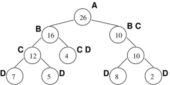
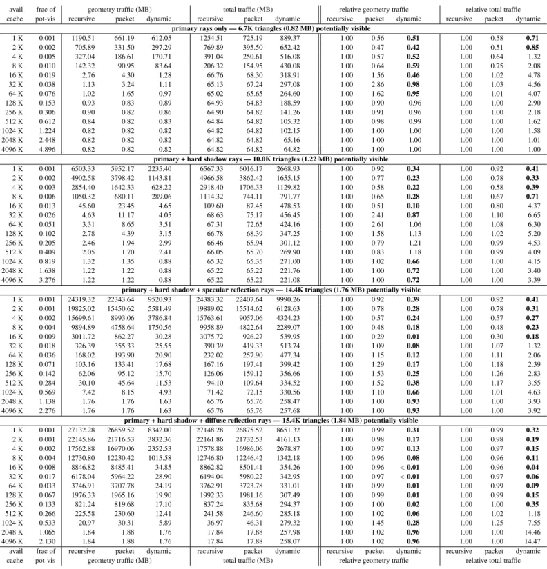
B 26 16 10 4 12 10 8 2 7 5 A B C D D C D D D C

Figure 1: Queue Point Selection — Here, we demonstrate how our queue point selection algorithm works on a toy k-d tree. We measure the amount of cache available to hold geometry and determine the

maximum amount of geometry (gmax) that can be loaded without

exceeding available cache capacity. We select the first node on each branch of the tree that contains geometry: g≤gmax. In this figure,

ifgmax≥26, the root (markedA) is the only queue point, and our

algorithm degenerates to Whitted-style ray tracing, because all ge-ometry fits in cache. If26>gmax≥16, the internal nodes markedB

are queue points. If16>_g_max≥10, theCnodes are queue points. If gmax≤10, the leaves (markedD) are queue points. Note that even

ifgmax is smaller than the amount of geometry at a leaf, that leaf

is made a queue point because there is no remaining acceleration structure beneath it (see Section 2.2).

queue point, there is a known, tight upper bound on the amount of data that must be touched to process all the rays in that queue.

Our algorithm seeks to optimize both (1) bandwidth utilization between main memory and the lowest level of processor cache and (2) utilization of the lowest level of processor cache itself. Without loss of generality, we will refer to DRAM-to-L2 bandwidth and L2 utilization in our discussion, since these are common components of the multi-core hardware that we target.

The algorithm described here uses a k-d tree as the acceleration structure, but it could be adapted to other acceleration structures, including regular grids, hierarchical grids, and bounding volume hierarchies. The ability of the acceleration structure to adapt to varying densities of scene geometry directly affects schedule qual-ity by limiting the flexibilqual-ity that we have in choosing queue points for rays. Our discussion will provide insight as to how the accel-eration structure interacts with other parts of the algorithm, but a thorough analysis of the impact of different acceleration structures is beyond the scope of this paper.

2.1 Traversal Algorithm

Our traversal algorithm traces rays from the root of the acceleration structure down to queue points, where further ray processing is de-ferred. It later iterates over these queue points to complete all ray traversals. To simplify our discussion, we first describe the traversal of primary rays only; then we generalize the discussion to handle secondary rays. See Section 2.2 for implementation details. 2.1.1 Traversing Primary Rays

We select queue points in the acceleration structure based on the amount of geometry that fits in available cache. Each queue point is the root of a subtree of the acceleration structure, a subtree that contains no more geometry than will fit into L2 cache. See Figure 1 for an example. If the entire scene fits into cache, then the root of the acceleration structure is the only queue point, and the traversal degenerates to Whitted’s recursive algorithm.

Our algorithm also efficiently schedules for worst-case condi-tions. Sometimes the construction of the acceleration structure can-not adapt to dense local geometry. At such points in a k-d tree, a leaf with an unusually large amount of geometry is placed in the acceleration structure. If the geometry at that leaf exceeds cache capacity, a recursive ray traversal willalwaysthrash the cacheeach

timesuch a leaf is pierced by a ray. Our algorithm treats such leaves as a separate scheduling problem, loading blocks of both rays and geometry to process the queue efficiently.

Our algorithm queues all primary rays, then iterates over the queues until all rays have terminated or have left the bounds of the scene. When a queue is processed, each ray traverses any of the re-maining subtree and is tested for intersection against the geometry at each leaf of the subtree that the ray might reach. Once a ray is se-lected at this stage, it is processed until either a successful intersec-tion is found or until the ray exits the bounds of the subtree. If the ray exits the bound of the subtree, it continues its traversal through the full acceleration structure, either to the next queue point or until it exits the bounds of the scene.

When a ray intersects a surface, we can either shade the inter-section point immediately (as in ray casting) or save it for deferred casting of secondary rays. A pixel id is maintained with the ray so that the proper pixel can be shaded. When supersampling, samples can be blended in the framebuffer as they arrive. If secondary rays are cast, then the point is shaded iteratively as each secondary ray is processed.

2.1.2 Traversing Secondary Rays

To handle secondary rays, our algorithm proceeds in generations: Shadow rays from the current generation are processed, then any newly spawned non-shadow rays are processed. By processing rays in generations, we limit the amount of active ray state in the system while still providing coherent access to scene geometry.

To generate shadow rays and other secondary rays, we maintain the intersection points for the current generation of rays. For each point light, we trace shadow rays from the light toward the inter-section points, which makes the traversal identical to the primary ray traversal method. Shadow rays inherit both the pixel id and the shading information from their spawning ray. Thus, when light vis-ibility has been determined, the shading contribution, if any, can be added to the appropriate pixel.

Once all shadow rays for the current generation have terminated, we traverse newly spawned non-shadow rays. Each new ray starts at the queue point that contains its origin. Our algorithm then iterates over queue points to traverse rays, as before. While our algorithm may achieve less coherence here than for primary and shadow rays, it can achieve better ray-object coherence than a recursive ray tracer by allowing many secondary rays to be active at once. Once all rays of this new generation have been processed, any resulting intersec-tion points are used to generate the next generaintersec-tion of shadow and secondary rays. This process continues until no new secondary rays are generated.

2.2 Implementation Sketch

We now describe how our algorithm can be implemented on a multi-core processor, assuming a 4MB L2 cache. We keep geom-etry and acceleration structure data cached while streaming rays to keep threads maximally occupied.

We represent k-d tree nodes using eight bytes, similar to the k-d tree used in PBRT [10]. We use an additional bit from the least-significant end of the mantissa of the split location to indi-cate whether a node is a queue point, leaving 20 bits for the single-precision mantissa representation. We expect this quantization to not significantly affect the quality of the k-d tree. With this repre-sentation, 128K nodes can remain resident if we reserve 1MB of the L2 for nodes. If the k-d tree is larger, we have the option of reserving more space or maintaining only the top of the tree, from the root down to the queue points. If we maintain only the top of the tree, we must load each subtree before processing its associated queue. This situation will only occur for extremely large scenes, where the added cost for loading the subtree will be insignificant compared to the cost of loading the associated geometry.

(3)

We also maintain a table that associates each queue point with a buffer in main memory that contains the actual ray queue. We keep this table and its associated buffers in memory so that rays can be enqueued quickly without having to load data to compute the address to which the ray should be sent. This table costs 8 bytes per entry, and we expect 32K queue points to be sufficient for most trees, so the table requires 256KB.

Rays must be cached to perform traversals and intersections, yet we expect to have hundreds to thousands of rays queued at each point. For example, if the camera point lies within the acceleration structure, all primary rays will begin in one queue. If we bring in too many rays, we evict other needed data from cache, so we buffer only enough rays to mask the latency of the initial cache miss on a leaf’s geometry. We know that all queued rays must be traversed through the active subtree, so this work will be available as long as there are queued rays. A single ray traversal step in a k-d tree is a ray-plane intersection test, made simpler because the plane is guaranteed to be axis-aligned. The ray-plane intersection test can be computed with a multiply, an add, and a comparison. With in-struction latency, the test takes about seven cycles to complete [14]. We estimate about ten traversal steps to take a ray from the queue point to a leaf. Assuming current DRAM latencies, two to four rays per thread should be sufficient to prevent idle threads.

We use a tight, 64-byte ray representation, with support for adap-tive sampling. Our ray layout supports up to 160-bit color, which must be included with each ray for linear processing. We include space for a pointer to adaptive sampling information, if required. We pad the structure to 64 bytes to maintain cache alignment.

Finally, we must cache geometry. We select queue points in the acceleration structure so that the geometry in the subtree will fit in available cache, taking into account the acceleration structure, ray buffer, etc., described above. We could load all geometry in the subtree immediately, but we cannot know which geometry, if any, will actually be required. To avoid spurious geometry loads, we lazily load geometry when a ray needs it for an intersection test. If a queue point is at a leaf, then we load the geometry immediately because it definitely will be tested for intersection.

For systems where cache resources are very limited, it is possi-ble to have a queue point at a leaf of the acceleration structure that contains more geometry than will fit in available cache. A Whitted-style ray tracer will thrash the cache each time a ray pierces such a leaf. Our algorithm permits more flexible approaches by treating this condition as a separate scheduling problem. The amount of ge-ometry at each leaf can be computed when building the acceleration structure, so we can detect a thrashing condition before loading any geometry. In such cases we create cache-sized blocks of geometry and iterate over them as we test for intersection against the rays in the ray buffer. This iterated processing technique results in fewer overall cache loads than uncontrolled cache thrashing.

3 Experimental Methodology

We now present results from an unoptimized ray tracer with a sim-ulated L2 cache. We evaluate the performance of our algorithm in terms of cache utilization and bandwidth consumption.

To obtain the cache measurements in our simulation, we create a memory trace with explicit reads and writes and run that trace through various cache configurations using Dinero IV [6], a light-weight trace-driven simulator. We simulate cache sizes in power-of-two increments from 1KB to 4MB, with 64B cache lines. This range of sizes allows us to measure the performance of our algo-rithm both when cache resources are scarce and when they are plen-tiful. Each cache is fully associative to eliminate conflict misses. Thus, after the cache is warm, all misses are capacity misses.

Our simulator is single-threaded, which eliminates multi-threaded cache issues, such as false sharing, from our measure-ments. In an optimized implementation, threads will

collabora-tively process the rays at a single queue point. Because the ge-ometry associated with each queue point fits in available cache, we expect to avoid most thread-related contention.

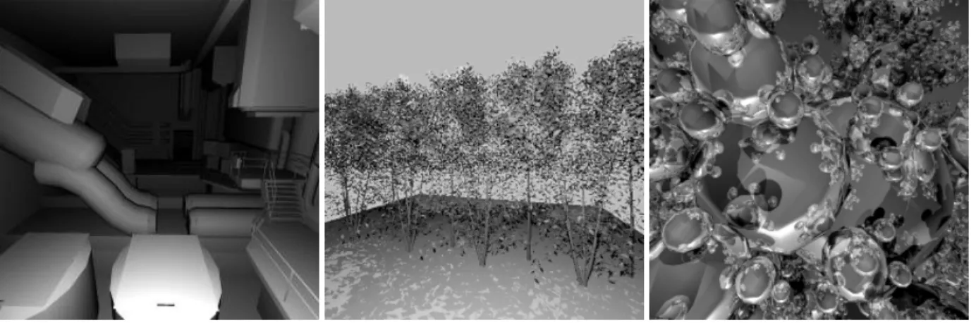
We test our algorithm on three scenes, shown in Figure 2. The scenes are rendered at 1024×1024 resolution for all runs except for diffuse reflections, where they are rendered at 512×512 resolu-tion. These models provide a variety of total geometry, potentially-visible geometry, and geometric topology. We use a small architec-tural scene (room: 47K triangles), a grove of tree models (grove: 164K triangles), and a four-level sphereflake model from the Stan-dard Procedural Database scenes [7] (sphereflake: 797K trian-gles). We specifically mention potentially-visible geometry when tracing primary and secondary rays because it more accurately mea-sures the geometry loaded when rendering. Total geometry affects the size and quality of the acceleration structure and whether the scene can fit in main memory, but it does not impact the geometry traffic between main memory and processor cache unless all geom-etry must be tested for intersection.

We compare our algorithm against two recursive ray tracers: A single-ray tracer using rays ordered along a Hilbert curve, and a ray packet tracer using 8×8 packets tiled over the image plane. We use a Hilbert curve ordering for single rays since this ordering is known to produce good image-plane coherence for rays [16]. We use an 8×8 packet size since it is the midpoint of currently popular packet sizes (4×4 [12, 18] — 16×16 [17]) and it was recently found to provide the most speed-up in this range [2].

4 Results and Discussion

This section shows that dynamic ray scheduling can improve cache utilization for geometry data by as much as an order of magnitude over recursive ray tracing. These savings will become increasingly important as additional lighting and shading data are stored in scene space, both increasing the amount of data that must be loaded and decreasing the available cache space for geometry.

4.1 Interpreting the Result Charts and Tables

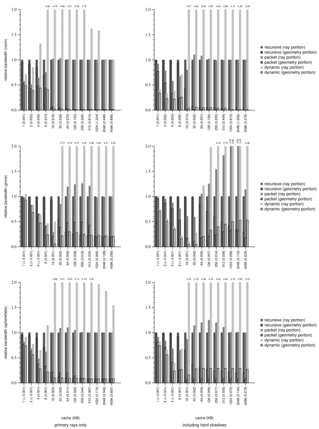
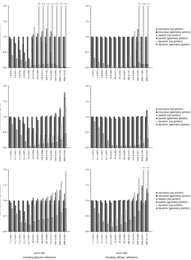
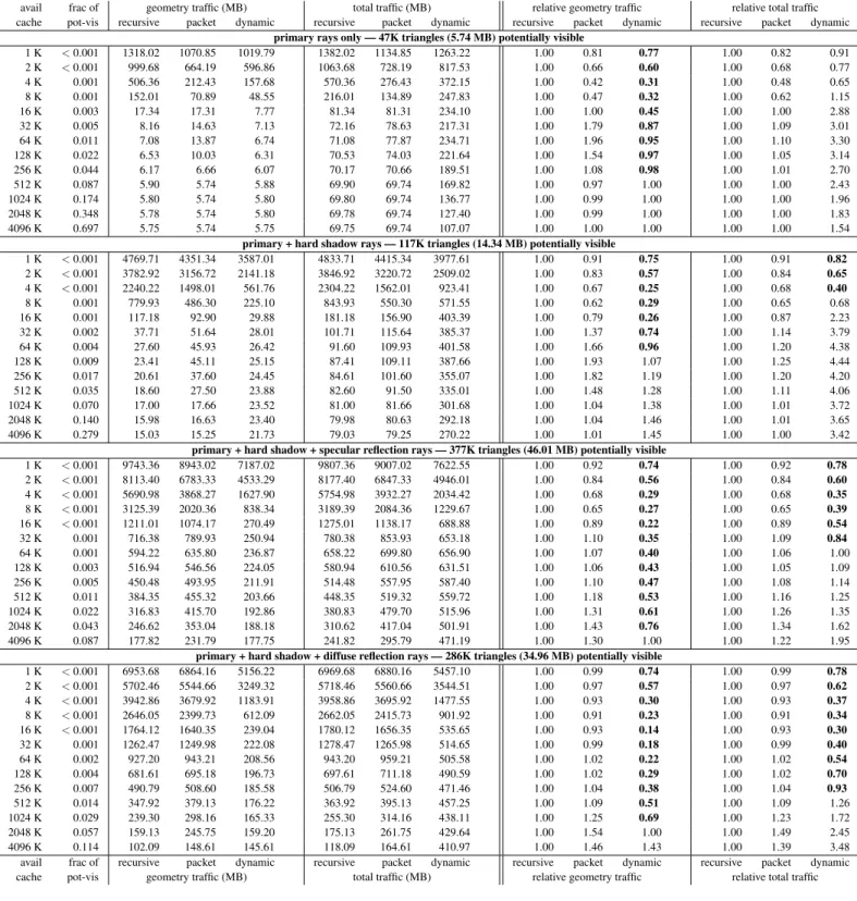
Figures 3–4 provide a comparison of our approach to both a single-ray tracer and a single-ray packet tracer. Figures 5–7 in the appendix show both the raw bandwidth measurements and the measurements normalized to the recursive ray tracer performance. Thus, smaller numbers represent a larger advantage for our algorithm. For exam-ple, 0.25 indicates a 4×bandwidth reduction over the recursive al-gorithm, 0.10 indicates a 10×reduction, and 0.01 indicates a 100× reduction.

For each scene/render configuration, we list the amount of ge-ometry that ispotentially visible. This is the amount of geometry that is tested for intersection against at least one ray, and thus it is the total amount of geometry that must be loaded into the cache. This amount represents the cache pressure from geometry more ac-curately than either total geometry or visible geometry, since total geometry includes geometry that is culled by the acceleration struc-ture and visible geometry omits geometry that is tested for intersec-tion but either is not hit or is occluded by other nearby geometry.

The tables include both the size of the available cache and the fraction of the potentially visible geometry that fits in that sized cache. This fraction expresses the cache pressure in the system for a particular combination of scene and cache size. Smaller values indicate greater pressure. Values greater than 1.0 indicate that all potentially visible geometry can be cached, which minimizes cache pressure. This fraction allows a fair comparison among scenes with different amounts of potentially visible geometry. Cache sizes that hold similar fractions of geometry should be compared (for exam-ple, 32K forroomand 512K for grove), rather than comparing results for the same cache sizes.

When tracing shadow rays, the amount of potentially visible ge-ometry differs slightly among our algorithm and the other

(4)

algo-Figure 2: Test scene images — We test our algorithm on three scenes: room,grove, andsphereflake. Note that the geometry artifacts in roomare contained in the scene specification and are not due to our ray tracer.

rithms. This is because shadow rays in our algorithm are traced from the light source to the non-shadow hit point, whereas in the other algorithms trace from hit point toward the light source. 4.2 Tracing Primary Rays

In Figures 5–7, we present our measurements for tracing primary rays only. These results show that our algorithm reduces geometry traffic between DRAM and L2 for all cache sizes at the cost of increased ray traffic. Ray traffic is more desirable than geometry traffic, since a thread must block for a geometry load but can switch to another ray if one is available. In other words, we want to keep geometry in cache and stream rays, as long as there are enough rays in cache to keep all threads busy.

Further, our algorithm significantly reduces geometry traffic when system resources are scarce. When the data load on the sys-tem is greatest, our algorithm adapts to make efficient use of avail-able resources. Recursive ray tracing cannot adapt in this way and thrashes the cache with geometry data. The problem is that recur-sive ray tracing maximally constrains the amount ofray trafficat the potential cost of increased geometry traffic. Our algorithm re-laxes this constraint, allowing ray traffic to grow while significantly reducing geometry traffic. Thus our algorithm can make efficient use of system resources and adapt to various system loads. 4.3 Tracing Secondary Rays

Our algorithm performs well when secondary rays are traced in ad-dition to primary rays. We present measurements for tracing pri-mary rays, shadow rays from three point-lights, specular reflections, and diffuse reflections. We separate the specular and diffuse reflec-tion cases to better observe their respective behavior. All reflecreflec-tions are limited to two bounces.

We use hemispherical sampling to generate diffuse reflection rays, similar to techniques used in Monte-Carlo global illumina-tion techniques and in photon-mapping [8]. Nine reflecillumina-tion rays are generated per sample, using a 3×3 sampling grid over the hemi-sphere. Each bounce has only a 10% chance of generating another sampling round. Our sampling is insufficient for accurate global illumination simulation, but it provides a reasonable approximation of system performance when tracing maximally incoherent rays.

In Figures 5–7, we show the extent to which our algorithm re-duces traffic from main memory to processor cache when tracing hard shadows and incoherent reflection rays (both specular and dif-fuse). The relative performance of our algorithmincreasesas ray incoherence and ray density increase, and the total data traffic of our algorithm never explodes as in the recursive algorithms.

Our algorithm performs best when visible geometry is large compared to available cache and when many rays are active at once. For example, on the 164K triangle grovescene rendered with hard shadows and diffuse reflections with 512KB cache avail-able, our algorithm reduces DRAM-to-L2 bandwidth consumption 7.8×compared to packet ray tracing. In contrast, on the 797K tri-anglesphereflakescene with the same configuration, our algo-rithm does not reduce bandwidth consumption because the scene is over-tessellated for the sampling rate used. Each sphere is at full resolution irrespective of the ray samples that access it. For such scenes, a multi-resolution system similar to Djeu et al. [5], with coarsification added, would boost our algorithm’s performance.

Our algorithm does comparatively worse when the working set of the recursive algorithm fits in available cache. However, we be-lieve these negative results will not translate into negative system performance because they only occur when much of the scene fits in cache. Further, recursive algorithms cannot maintain locality un-der complex lighting models. Global illumination approximations can generate tens to hundreds of secondary rays per primary ray, each of which may access new, uncached geometry. A recursive ray tracer will eventually thrash the cache with geometry data, whereas our algorithm will continue to process these rays coherently. 5 Related Work

As mentioned earlier, our work builds on several previous ray scheduling schemes to create an algorithm in which both geome-try and rays are actively managed. We now discuss this and other related work to better distinguish the contributions of our algorithm. All recursive ray tracers implement some form of Whitted’s orig-inal recursive ray tracing algorithm [20]. Recent innovations to the basic algorithm include the use of SIMD instructions to trace multiple rays in parallel [19] and the tracing of a frustum of rays through the acceleration structure to eliminate upper level traver-sal steps [12]. These techniques can increase the number of rays active in the system at once, but they do not allow rays to be dy-namically scheduled: Once a ray (or packet of rays) is selected for traversal, the selected ray(s)and all child raysmust be traced to completion before another selection choice is made. The fixed ac-tive ray state in these algorithms hampers their ability to prevent thrashing or to effectively hide latency. Recently, Boulos et al. [2], attempted to achieve real-time frame rates on a current workstation-class system for both Whitted-style ray tracing with full specular effects and distribution ray tracing [3], but without ray schedul-ing. They achieve interactive rates for their Whitted-style tracer for both primary and secondary rays by employing clever methods of organizing secondary rays. Further, Boulos et al., observe that

(5)

1 (0.001) 2 (0.002) 4 (0.005) 8 (0.010) 16 (0.019) 32 (0.038) 64 (0.076) 128 (0.153) 256 (0.306) 512 (0.612) 1024 (1.224) 2048 (2.448) 4096 (4.896) 0.0 0.5 1.0 1.5 2.0

relative bandwidth (room)

2.08 4.784.56 4.07 2.90 2.18 1 (0.001) 2 (0.002) 4 (0.003) 8 (0.006) 16 (0.013) 32 (0.026) 64 (0.051) 128 (0.102) 256 (0.205) 512 (0.409) 1024 (0.819) 2048 (1.638) 4096 (3.276) 0.0 0.5 1.0 1.5 2.0

recursive (ray portion) recursive (geometry portion) packet (ray portion) packet (geometry portion) dynamic (ray portion) dynamic (geometry portion) 4.37 6.65 6.30 5.20 4.534.09 4.15 3.40 3.39 1 (< 0.001) 2 (< 0.001) 4 (< 0.001) 8 (0.001) 16 (0.001) 32 (0.002) 64 (0.004) 128 (0.008) 256 (0.016) 512 (0.032) 1024 (0.065) 2048 (0.129) 4096 (0.258) 0.0 0.5 1.0 1.5 2.0

relative bandwidth (grove)

2.73 3.72 3.51 3.042.58 2.44 2.31 2.20 1 (< 0.001) 2 (< 0.001) 4 (< 0.001) 8 (< 0.001) 16 (0.001) 32 (0.002) 64 (0.003) 128 (0.007) 256 (0.014) 512 (0.028) 1024 (0.056) 2048 (0.112) 4096 (0.224) 0.0 0.5 1.0 1.5 2.0

recursive (ray portion) recursive (geometry portion) packet (ray portion) packet (geometry portion) dynamic (ray portion) dynamic (geometry portion) 2.02 2.02 2.542.75 3.06 3.33 3.46 1 (< 0.001) 2 (< 0.001) 4 (0.001) 8 (0.001) 16 (0.003) 32 (0.005) 64 (0.011) 128 (0.022) 256 (0.044) 512 (0.087) 1024 (0.174) 2048 (0.348) 4096 (0.697) cache (KB) 0.0 0.5 1.0 1.5 2.0

relative bandwidth (sphereflake)

primary rays only 2.883.01 3.30 3.14 2.702.43 1 (< 0.001) 2 (< 0.001) 4 (< 0.001) 8 (0.001) 16 (0.001) 32 (0.002) 64 (0.004) 128 (0.009) 256 (0.017) 512 (0.035) 1024 (0.070) 2048 (0.140) 4096 (0.279) cache (KB) 0.0 0.5 1.0 1.5 2.0

including hard shadows

recursive (ray portion) recursive (geometry portion) packet (ray portion) packet (geometry portion) dynamic (ray portion) dynamic (geometry portion) 2.23 3.79 4.38 4.44 4.204.06 3.72 3.65 3.42

Figure 3: Relative traffic from main memory to processor cache for primary rays only and including hard shadows — These charts show relative bandwidth traffic, normalized to single-ray recursive performance, for primary rays only and for primary rays plus hard shadow rays. Numbers less than one indicate better bandwidth utilization compared to single-ray recursive tracing. The total bar height represents total relative bandwidth used. The lower bar portion represents the bandwidth used for geometry data, and the upper bar portion represents bandwidth used for ray data. Note that the charts are bounded at2.0. Please refer to Figure5–7 for the underlying data.

(6)

1 (0.001) 2 (0.001) 4 (0.002) 8 (0.004) 16 (0.009) 32 (0.018) 64 (0.036) 128 (0.071) 256 (0.142) 512 (0.284) 1024 (0.569) 2048 (1.138) 4096 (2.276) 0.0 0.5 1.0 1.5 2.0

relative bandwidth (room)

2.06 2.39 2.833.55 4.63 3.93 3.92 1 (0.001) 2 (0.001) 4 (0.002) 8 (0.004) 16 (0.008) 32 (0.017) 64 (0.033) 128 (0.067) 256 (0.133) 512 (0.266) 1024 (0.533) 2048 (1.065) 4096 (2.130) 0.0 0.5 1.0 1.5 2.0

recursive (ray portion) recursive (geometry portion) packet (ray portion) packet (geometry portion) dynamic (ray portion) dynamic (geometry portion) 7.55 14.46 14.47 1 (< 0.001) 2 (< 0.001) 4 (< 0.001) 8 (< 0.001) 16 (0.001) 32 (0.002) 64 (0.003) 128 (0.006) 256 (0.013) 512 (0.025) 1024 (0.051) 2048 (0.102) 4096 (0.204) 0.0 0.5 1.0 1.5 2.0

relative bandwidth (grove)

1 (< 0.001) 2 (< 0.001) 4 (< 0.001) 8 (< 0.001) 16 (0.001) 32 (0.002) 64 (0.003) 128 (0.006) 256 (0.013) 512 (0.025) 1024 (0.051) 2048 (0.102) 4096 (0.204) 0.0 0.5 1.0 1.5 2.0

recursive (ray portion) recursive (geometry portion) packet (ray portion) packet (geometry portion) dynamic (ray portion) dynamic (geometry portion)

1 (< 0.001) 2 (< 0.001) 4 (< 0.001) 8 (< 0.001) 16 (< 0.001) 32 (0.001) 64 (0.001) 128 (0.003) 256 (0.005) 512 (0.011) 1024 (0.022) 2048 (0.043) 4096 (0.087) cache (KB) 0.0 0.5 1.0 1.5 2.0

relative bandwidth (sphereflake)

including specular reflections

1 (< 0.001) 2 (< 0.001) 4 (< 0.001) 8 (< 0.001) 16 (< 0.001) 32 (0.001) 64 (0.002) 128 (0.004) 256 (0.007) 512 (0.014) 1024 (0.029) 2048 (0.057) 4096 (0.114) cache (KB) 0.0 0.5 1.0 1.5 2.0 including_diffuse_reflections

recursive (ray portion) recursive (geometry portion) packet (ray portion) packet (geometry portion) dynamic (ray portion) dynamic (geometry portion) 2.45 3.48

Figure 4: Relative traffic from main memory to processor cache including specular reflections and including diffuse reflections — These charts show relative bandwidth traffic, normalized to single-ray recursive performance, for primary rays, hard shadow rays, and reflections. Numbers less than one indicate better bandwidth utilization compared to single-ray recursive tracing. The total bar height represents total relative bandwidth used. The lower bar portion represents the bandwidth used for geometry data, and the upper bar portion represents bandwidth used for ray data. Note that the charts are bounded at2.0. Please refer to Figure5–7 for the underlying data.

(7)

shading computation may soon overtake visibility computation as the primary system cost. Note that our algorithm could accept a modified form of their secondary ray organization technique. Also, because our algorithm operates in local regions of scene space, it facilitates the grouping of similarly shaded points, making efficient use of shading computation.

Pharr et al. [11], take an approach quite different from the Whit-ted tracing model. Their ray scheduling algorithm permits ray re-ordering by using a linear formulation of the rendering equation [9], where the outgoing radiance is the weighted sum of the incoming radiances. This formulation computes radiance as rays are traced rather than accumulating it on the recursion stack. Pharr et al.’s al-gorithm targets efficient use of main memory and traffic between disk and RAM to render models that cannot fit in main memory. Pharr et al. use Monte-Carlo-based global illumination to model indirect diffuse lighting, a technique that uses many sample rays per primary ray.

Since Pharr et al.’s algorithm targets a higher level of the memory hierarchy, there are aspects of it that are poorly suited for RAM-to-cache traffic. The acceleration structure is a uniform grid, which, because it is non-adaptive, makes it difficult to constrain the amount of geometry at any particular cell. This variance can be masked at the RAM level, but at the cache level it complicates effective scheduling. Also, while rays can be reordered under Pharr et al.’s algorithm, the number of active rays is not bounded. Instead, the algorithm actively seeks to get deep into the ray tree quickly, so many secondary rays of many ray generations are active in the sys-tem at once. Again, while this technique may be effective when considering disk to RAM traffic, the ray state explosion that results can cause serious thrashing in cache-sized memories. Our tech-nique controls both geometry state and ray state to ensure efficient operation within a given system.

We are aware of two implementations of algorithms similar to that of Pharr et al. Dachille and Kaufman [4] used Pharr et al.’s ray deferring algorithm in a hardware-based volume rendering sys-tem. They use specialized hardware to perform standard volume rendering and volume rendering with a simplified global illumina-tion model. In this system, rays are collected at each cell of the volume, much the way that rays are collected in Pharr et al.’s uni-form grid. Cells are then scheduled for processing as in Pharr et al.’s algorithm. They were able to achieve interactive frame rates on a simulation of their hardware. Because they use direct volume rendering, there is no significant geometry traffic per cell: The sys-tem loads the eight vertices of the cell and trilinearly interpolates each sample along each ray. Thus, their system does not manage geometry traffic at all. Steinhurst et al. [15], use Pharr-like reorder-ing to obtain better cache performance for photon mappreorder-ing. Like Pharr et al., their system experiences ray state explosion. However, its effects cannot be masked at the cache level, and the performance of their system suffers. We expect that our algorithm would per-form better on this task because it actively manages ray state, and our results on diffuse reflection rays support this expectation. 6 Conclusions and Future Work

We have presented a ray tracing algorithm that dynamically sched-ules rays in order to actively manage both ray and geometry data. In so doing, our algorithm significantly reduces geometry traffic be-tween DRAM and L2 cache with a moderate increase in ray traffic. Our algorithm dramatically reduces bandwidth consumed between main memory and processor cachewhen cache resources are scarce andwhen the scene is highly sampled, thus permitting the efficient ray tracing of large, complex scenes.

We have three areas for future work. First, we will expand our re-search ray tracer to include other ray-based algorithms such as pho-ton mapping [8] and distribution ray tracing effects [3]. Second, we will investigate different ray scheduling methods that may further

reduce bandwidth consumption. Third, we will complete the op-timized implementation of our system as described in Section 2.2, which will target the latest multi-core multi-threaded commodity architecture.

Acknowledgments

Thanks to Peter Djeu, the Real-Time Graphics and Systems group at UT, and the anonymous reviewers for their insight and helpful comments. Special thanks to Jim Hurley and Stephen Junkins at Intel for their enthusiastic support of ray tracing research. This re-search was supported in part by NSF grants EIA-0303609, ACI-0313263, ACI-9984660 and CCF-0546236; by a grant from the In-tel Research Council; and by a fellowship from the IC2Institute at UT-Austin.

References

[1] C. Benthin, I. Wald, M. Scherbaum, and H. Friedrich. Ray Tracing on the CELL Processor. InProceedings of the 2006 IEEE Symposium on

Interactive Ray Tracing, pages 25–23, 2006.

[2] S. Boulos, D. Edwards, J. D. Lacewell, J. Kniss, J. Kautz, I. Wald, and P. Shirley. Packet-Based Whitted and Distribution Ray Tracing. In

Proceedings of Graphics Interface 2007, 2007.

[3] R. L. Cook, T. Porter, and L. Carpenter. Distributed Ray Tracing. In

Proceedings of SIGGRAPH 84, pages 137–145, 1984.

[4] F. Dachille IX and A. Kaufman. GI-Cube: An Architecture for Volu-metric Global Illumination and Rendering. In2000 SIGGRAPH /

Eu-rographics Workshop on Graphics Hardware, pages 119–128, 2000.

[5] P. Djeu, W. Hunt, R. Wang, I. Elhassan, G. Stoll, and W. R. Mark. Razor: An architecture for dynamic multiresolution ray tracing.ACM

Transactions on Graphics (conditionally accepted), 2007.

[6] J. Edler and M. D. Hill. Dinero IV cache simulator (http://www.cs.wisc.edu/∼markhill/DineroIV/), 1998.

[7] E. A. Haines. A Proposal for Standard Graphics Environments.IEEE

Computer Graphics & Applications, 7(11):3–5, 1987.

[8] H. W. Jensen. Global Illumination using Photon Maps. In

Eurograph-ics Rendering Workshop 1996, pages 21–30, 1996.

[9] J. T. Kajiya. The Rendering Equation. InProceedings of SIGGRAPH, pages 143–150, 1986.

[10] M. Pharr and G. Humphreys.Physically Based Rendering: From

The-ory to Implementation. Morgan Kaufmann, 2004.

[11] M. Pharr, C. Kolb, R. Gershbein, and P. M. Hanrahan. Rendering Complex Scenes with Memory-Coherent Ray Tracing. InProceedings

of SIGGRAPH, pages 101–108, 1997.

[12] A. Reshetov, A. Soupikov, and J. Hurley. Multi-Level Ray Tracing Algorithm.Proceedings of SIGGRAPH, 24(3):1176–1185, 2005. [13] J. Schmittler, S. Woop, D. Wagner, P. Slusallek, and W. J. Paul.

Real-time Ray Tracing of Dynamic Scenes on an FPGA Chip. InGraphics

Hardware 2004, pages 95–106, 2004.

[14] P. Slusallek, P. Shirley, W. Mark, G. Stoll, and I. Wald. Parallel & Distributed Processing. InACM SIGGRAPH 2005 Courses, 2005. [15] J. Steinhurst, G. Coombe, and A. Lastra. Reordering for Cache

Con-scious Photon Mapping. InProceedings of GI, pages 97–104, 2005. [16] D. Voorhies. Space-Filling Curves and a Measure of Coherence. In

Graphics Gems II, pages 26–30, 485–486. 1991.

[17] I. Wald, S. Boulos, and P. Shirley. Ray Tracing Deformable Scenes Using Dynamic Bounding Volume Hierarchies.ACM Transactions on

Graphics, 26(1):6, 2007.

[18] I. Wald, T. Ize, A. Kensler, A. Knoll, and S. G. Parker. Ray Trac-ing Animated Scenes UsTrac-ing Coherent Grid Traversal.Proceedings of

SIGGRAPH, 25(3):485–493, 2006.

[19] I. Wald, P. Slusallek, C. Benthin, and M. Wagner. Interactive Ren-dering with Coherent Ray Tracing. Computer Graphics Forum, 20(3):153–164, 2001.

[20] T. Whitted. An Improved Illumination Model for Shaded Display.

Communications of the ACM, 6(23):343–349, 1980.

[21] S. Woop, J. Schmittler, and P. Slusallek. RPU: a programmable ray processing unit for realtime ray tracing.ACM Transactions on Graph-ics, 24(3):434–444, 2005.

(8)

room — 47K triangles (5.76 MB)

avail frac of geometry traffic (MB) total traffic (MB) relative geometry traffic relative total traffic cache pot-vis recursive packet dynamic recursive packet dynamic recursive packet dynamic recursive packet dynamic

primary rays only — 6.7K triangles (0.82 MB) potentially visible

1 K 0.001 1190.51 661.19 612.05 1254.51 725.19 889.37 1.00 0.56 0.51 1.00 0.58 0.71 2 K 0.002 705.89 331.50 297.29 769.89 395.50 652.42 1.00 0.47 0.42 1.00 0.51 0.85 4 K 0.005 327.04 186.61 170.71 391.04 250.61 516.08 1.00 0.57 0.52 1.00 0.64 1.32 8 K 0.010 142.32 90.95 83.64 206.32 154.95 430.08 1.00 0.64 0.59 1.00 0.75 2.08 16 K 0.019 2.76 4.30 1.28 66.76 68.30 318.91 1.00 1.56 0.46 1.00 1.02 4.78 32 K 0.038 1.13 3.24 1.11 65.13 67.24 297.08 1.00 2.86 0.98 1.00 1.03 4.56 64 K 0.076 1.02 1.65 0.97 65.02 65.65 264.60 1.00 1.62 0.95 1.00 1.01 4.07 128 K 0.153 0.93 0.83 0.89 64.93 64.83 188.59 1.00 0.90 0.96 1.00 1.00 2.90 256 K 0.306 0.90 0.82 0.86 64.90 64.82 141.26 1.00 0.91 0.96 1.00 1.00 2.18 512 K 0.612 0.84 0.82 0.83 64.84 64.82 105.32 1.00 0.98 0.99 1.00 1.00 1.62 1024 K 1.224 0.82 0.82 0.82 64.82 64.82 102.15 1.00 1.00 1.00 1.00 1.00 1.58 2048 K 2.448 0.82 0.82 0.82 64.82 64.82 65.16 1.00 1.00 1.00 1.00 1.00 1.01 4096 K 4.896 0.82 0.82 0.82 64.82 64.82 64.82 1.00 1.00 1.00 1.00 1.00 1.00

primary + hard shadow rays — 10.0K triangles (1.22 MB) potentially visible

1 K 0.001 6503.33 5952.17 2235.40 6567.33 6016.17 2668.93 1.00 0.92 0.34 1.00 0.92 0.41 2 K 0.002 4902.58 3798.42 1143.81 4966.58 3862.42 1655.15 1.00 0.77 0.23 1.00 0.78 0.33 4 K 0.003 2854.40 1642.33 628.22 2918.40 1706.33 1129.82 1.00 0.58 0.22 1.00 0.58 0.39 8 K 0.006 1050.32 680.11 289.06 1114.32 744.11 791.77 1.00 0.65 0.28 1.00 0.67 0.71 16 K 0.013 45.60 23.45 4.65 109.60 87.45 478.53 1.00 0.51 0.10 1.00 0.80 4.37 32 K 0.026 4.63 11.17 4.05 68.63 75.17 456.45 1.00 2.41 0.87 1.00 1.10 6.65 64 K 0.051 3.31 8.65 3.51 67.31 72.65 424.16 1.00 2.61 1.06 1.00 1.08 6.30 128 K 0.102 2.78 4.39 3.15 66.78 68.39 347.25 1.00 1.58 1.13 1.00 1.02 5.20 256 K 0.205 2.46 1.94 2.99 66.46 65.94 301.12 1.00 0.79 1.21 1.00 0.99 4.53 512 K 0.409 2.05 1.70 2.41 66.05 65.70 269.90 1.00 0.83 1.18 1.00 0.99 4.09 1024 K 0.819 1.32 1.35 0.88 65.32 65.35 271.00 1.00 1.02 0.66 1.00 1.00 4.15 2048 K 1.638 1.22 1.22 0.88 65.22 65.22 221.76 1.00 1.00 0.72 1.00 1.00 3.40 4096 K 3.276 1.22 1.22 0.88 65.22 65.22 221.08 1.00 1.00 0.72 1.00 1.00 3.39

primary + hard shadow + specular reflection rays — 14.4K triangles (1.76 MB) potentially visible

1 K 0.001 24319.32 22343.64 9520.93 24383.32 22407.64 9990.26 1.00 0.92 0.39 1.00 0.92 0.41 2 K 0.001 19825.02 15450.62 5581.49 19889.02 15514.62 6128.63 1.00 0.78 0.28 1.00 0.78 0.31 4 K 0.002 15699.61 8993.06 3786.84 15763.61 9057.06 4324.23 1.00 0.57 0.24 1.00 0.57 0.27 8 K 0.004 9894.89 4758.64 1750.56 9958.89 4822.64 2289.07 1.00 0.48 0.18 1.00 0.48 0.23 16 K 0.009 3011.72 862.27 30.28 3075.72 926.27 539.95 1.00 0.29 0.01 1.00 0.30 0.18 32 K 0.018 326.39 355.33 25.55 390.39 419.33 513.74 1.00 1.09 0.08 1.00 1.07 1.32 64 K 0.036 168.02 193.90 20.90 232.02 257.90 477.34 1.00 1.15 0.12 1.00 1.11 2.06 128 K 0.071 103.16 133.41 17.68 167.16 197.41 399.42 1.00 1.29 0.17 1.00 1.18 2.39 256 K 0.142 62.06 95.12 15.70 126.06 159.12 356.66 1.00 1.53 0.25 1.00 1.26 2.83 512 K 0.284 30.10 45.64 11.53 94.10 109.64 334.52 1.00 1.52 0.38 1.00 1.17 3.55 1024 K 0.569 7.42 8.15 4.93 71.42 72.15 330.56 1.00 1.10 0.66 1.00 1.01 4.63 2048 K 1.138 1.76 1.76 1.63 65.76 65.76 258.47 1.00 1.00 0.93 1.00 1.00 3.93 4096 K 2.276 1.76 1.76 1.63 65.76 65.76 257.68 1.00 1.00 0.93 1.00 1.00 3.92

primary + hard shadow + diffuse reflection rays — 15.4K triangles (1.84 MB) potentially visible

1 K 0.001 27132.28 26859.52 8342.00 27148.28 26875.52 8651.32 1.00 0.99 0.31 1.00 0.99 0.32 2 K 0.001 22145.86 21716.53 3832.36 22161.86 21732.53 4161.13 1.00 0.98 0.17 1.00 0.98 0.19 4 K 0.002 17562.88 16970.06 2352.53 17578.88 16986.06 2678.87 1.00 0.97 0.13 1.00 0.97 0.15 8 K 0.004 12730.80 12230.42 1015.58 12746.80 12246.42 1342.18 1.00 0.96 0.08 1.00 0.96 0.11 16 K 0.008 8846.82 8485.41 34.85 8862.82 8501.41 354.26 1.00 0.96 <0.01 1.00 0.96 0.04 32 K 0.017 6178.04 5964.22 28.90 6194.04 5980.22 342.95 1.00 0.97 <0.01 1.00 0.97 0.06 64 K 0.033 3746.91 3707.78 24.19 3762.91 3723.78 331.01 1.00 0.99 0.01 1.00 0.99 0.09 128 K 0.067 1976.33 1965.16 19.90 1992.33 1981.16 307.49 1.00 0.99 0.01 1.00 0.99 0.15 256 K 0.133 821.24 819.68 17.10 837.24 835.68 294.37 1.00 1.00 0.02 1.00 1.00 0.35 512 K 0.266 225.58 230.60 12.41 241.58 246.60 285.18 1.00 1.02 0.06 1.00 1.02 1.18 1024 K 0.533 20.97 30.31 5.89 36.97 46.31 279.32 1.00 1.45 0.28 1.00 1.25 7.55 2048 K 1.065 1.84 1.88 1.76 17.84 17.88 257.98 1.00 1.02 0.96 1.00 1.00 14.46 4096 K 2.130 1.84 1.88 1.76 17.84 17.88 258.07 1.00 1.02 0.96 1.00 1.00 14.47 avail frac of recursive packet dynamic recursive packet dynamic recursive packet dynamic recursive packet dynamic cache pot-vis geometry traffic (MB) total traffic (MB) relative geometry traffic relative total traffic

Figure 5: Traffic from main memory to processor cache forroom — Even on our smallest test scene, both in total geometry and in visible geometry, our algorithm reduces geometry traffic. The most dramatic traffic reduction comes at the smaller tested cache sizes. For diffuse reflection rays, when rays are maximally incoherent, we can reduce geometry traffic by as much astwo orders of magnitude(16K – 128K) and total traffic by as much as an order of magnitude. When the working set for the recursive algorithm fits in available cache, the relative performance of our algorithm suffers because of the overhead to maintain the ray queues. Note that while our relative performance numbers are worse for these resource-plentiful situations, the total bandwidth consumed is relatively low, so the impact on system performance is small.

(9)

grove — 164K triangles (20.11 MB)

primary rays only — 127K triangles (15.49 MB) potentially visible

1 K <0.001 4878.67 4759.77 4611.01 4942.67 4823.77 5198.92 1.00 0.98 0.95 1.00 0.98 1.05 2 K <0.001 3940.24 3274.72 2730.68 4004.24 3338.72 3310.41 1.00 0.83 0.69 1.00 0.83 0.83 4 K <0.001 3091.94 2006.40 1478.22 3155.94 2070.40 2011.84 1.00 0.65 0.48 1.00 0.66 0.64 8 K 0.001 2112.50 874.21 512.41 2176.50 938.21 993.60 1.00 0.41 0.24 1.00 0.43 0.46 16 K 0.001 839.94 194.23 58.30 903.94 258.23 455.63 1.00 0.23 0.07 1.00 0.29 0.50 32 K 0.002 75.01 53.69 30.61 139.01 117.69 378.94 1.00 0.72 0.41 1.00 0.85 2.73 64 K 0.004 25.63 42.82 26.71 89.63 106.82 333.69 1.00 1.67 1.04 1.00 1.19 3.72 128 K 0.008 21.60 42.18 23.66 85.60 106.18 300.77 1.00 1.95 1.10 1.00 1.24 3.51 256 K 0.016 19.21 40.68 20.53 83.21 104.68 252.69 1.00 2.12 1.07 1.00 1.26 3.04 512 K 0.032 17.78 35.07 19.08 81.78 99.07 211.12 1.00 1.97 1.07 1.00 1.21 2.58 1024 K 0.065 16.81 15.53 18.27 80.81 79.53 197.00 1.00 0.92 1.09 1.00 0.98 2.44 2048 K 0.129 16.26 15.49 17.39 80.26 79.49 185.47 1.00 0.95 1.07 1.00 0.99 2.31 4096 K 0.258 15.89 15.49 16.38 79.89 79.49 175.73 1.00 0.97 1.03 1.00 1.00 2.20

primary + hard shadow rays — 146K triangles (17.86 MB) potentially visible

1 K <0.001 16456.48 16369.24 11761.99 16520.48 16433.24 12377.85 1.00 0.99 0.71 1.00 0.99 0.75 2 K <0.001 13453.69 12751.53 6939.68 13517.69 12815.53 7547.35 1.00 0.95 0.52 1.00 0.95 0.56 4 K <0.001 10932.37 9541.58 3831.61 10996.37 9605.58 4393.17 1.00 0.87 0.35 1.00 0.87 0.40 8 K <0.001 8349.56 6299.49 1335.52 8413.56 6363.49 1888.32 1.00 0.75 0.16 1.00 0.76 0.22 16 K 0.001 5205.51 3135.72 185.01 5269.51 3199.72 653.95 1.00 0.60 0.04 1.00 0.61 0.12 32 K 0.002 1747.25 1005.87 94.37 1811.25 1069.87 514.31 1.00 0.58 0.05 1.00 0.59 0.28 64 K 0.003 312.82 331.45 80.48 376.82 395.45 459.08 1.00 1.06 0.26 1.00 1.05 1.22 128 K 0.007 147.59 200.51 70.20 211.59 264.51 418.93 1.00 1.36 0.48 1.00 1.25 1.98 256 K 0.014 93.47 179.10 63.12 157.47 243.10 399.26 1.00 1.92 0.68 1.00 1.54 2.54 512 K 0.028 64.60 169.80 58.19 128.60 233.80 354.22 1.00 2.63 0.90 1.00 1.82 2.75 1024 K 0.056 46.52 159.46 55.15 110.52 223.46 337.96 1.00 3.43 1.19 1.00 2.02 3.06 2048 K 0.112 33.44 132.42 51.85 97.44 196.42 324.04 1.00 3.96 1.55 1.00 2.02 3.33 4096 K 0.224 26.15 38.64 48.00 90.15 102.64 311.68 1.00 1.48 1.84 1.00 1.14 3.46

primary + hard shadow + specular reflection rays — 161K triangles (19.65 MB) potentially visible

1 K <0.001 32234.51 32097.76 24307.08 32298.51 32161.76 25086.99 1.00 1.00 0.75 1.00 1.00 0.78 2 K <0.001 26554.50 25509.81 15047.44 26618.50 25573.81 15819.16 1.00 0.96 0.57 1.00 0.96 0.59 4 K <0.001 21971.56 19602.54 8632.18 22035.56 19666.54 9357.80 1.00 0.89 0.39 1.00 0.89 0.42 8 K <0.001 17897.54 13787.43 3357.71 17961.54 13851.43 4030.91 1.00 0.77 0.19 1.00 0.77 0.22 16 K 0.001 13488.00 8555.37 717.55 13552.00 8619.37 1306.88 1.00 0.63 0.05 1.00 0.64 0.10 32 K 0.002 8413.83 5266.98 456.06 8477.83 5330.98 996.39 1.00 0.63 0.05 1.00 0.63 0.12 64 K 0.003 4141.86 3720.42 378.81 4205.86 3784.42 877.79 1.00 0.90 0.09 1.00 0.90 0.21 128 K 0.006 2658.29 2744.06 318.88 2722.29 2808.06 787.99 1.00 1.03 0.12 1.00 1.03 0.29 256 K 0.013 2053.98 2146.78 279.52 2117.98 2210.78 703.68 1.00 1.05 0.14 1.00 1.04 0.33 512 K 0.025 1587.80 1676.14 248.25 1651.80 1740.14 632.31 1.00 1.06 0.16 1.00 1.05 0.38 1024 K 0.051 1149.28 1302.49 224.13 1213.28 1366.49 594.96 1.00 1.13 0.20 1.00 1.13 0.49 2048 K 0.102 715.54 943.60 202.18 779.54 1007.60 562.51 1.00 1.32 0.28 1.00 1.29 0.72 4096 K 0.204 332.24 644.69 179.82 396.24 708.69 531.92 1.00 1.94 0.54 1.00 1.79 1.34

primary + hard shadow + diffuse reflection rays — 161K triangles (19.62 MB) potentially visible

1 K <0.001 23581.31 23567.99 19718.37 23597.31 23583.99 20105.27 1.00 1.00 0.84 1.00 1.00 0.85 2 K <0.001 19448.90 19350.91 12368.50 19464.90 19366.91 12753.37 1.00 0.99 0.64 1.00 0.99 0.66 4 K <0.001 16195.96 15946.00 7247.89 16211.96 15962.00 7621.18 1.00 0.98 0.45 1.00 0.98 0.47 8 K <0.001 13492.55 13017.76 3037.43 13508.55 13033.76 3397.65 1.00 0.96 0.23 1.00 0.96 0.25 16 K 0.001 11276.60 10581.27 801.17 11292.60 10597.27 1140.42 1.00 0.94 0.07 1.00 0.94 0.10 32 K 0.002 9654.98 8963.49 539.21 9670.98 8979.49 866.23 1.00 0.93 0.06 1.00 0.93 0.09 64 K 0.003 8359.51 7950.33 440.57 8375.51 7966.33 757.26 1.00 0.95 0.05 1.00 0.95 0.09 128 K 0.006 7013.85 6892.24 360.19 7029.85 6908.24 669.42 1.00 0.98 0.05 1.00 0.98 0.10 256 K 0.013 5741.27 5687.78 315.06 5757.27 5703.78 613.09 1.00 0.99 0.05 1.00 0.99 0.11 512 K 0.025 4435.86 4393.57 276.74 4451.86 4409.57 564.75 1.00 0.99 0.06 1.00 0.99 0.13 1024 K 0.051 3008.07 3055.72 245.21 3024.07 3071.72 529.93 1.00 1.02 0.08 1.00 1.02 0.18 2048 K 0.102 1631.21 1682.71 218.59 1647.21 1698.71 500.76 1.00 1.03 0.13 1.00 1.03 0.30 4096 K 0.204 615.06 748.40 182.56 631.06 764.40 463.14 1.00 1.22 0.30 1.00 1.21 0.73 avail frac of recursive packet dynamic recursive packet dynamic recursive packet dynamic recursive packet dynamic cache pot-vis geometry traffic (MB) total traffic (MB) relative geometry traffic relative total traffic

Figure 6: Traffic from main memory to processor cache forgrove— On this larger test scene, the benefit of our algorithm becomes clear. When cache resources are scarce, our algorithm significantly reduces data traffic. When cache resources are plentiful our algorithm achieves better cache utilization with respect to geometry, at the cost of increased ray traffic. The results for incoherent rays (specular and diffuse reflections) are particularly striking, where our algorithm significantly reduces total data traffic even with megabytes of available cache.

(10)

sphereflake — 797K triangles (97.31 MB)

primary rays only — 47K triangles (5.74 MB) potentially visible

1 K <0.001 1318.02 1070.85 1019.79 1382.02 1134.85 1263.22 1.00 0.81 0.77 1.00 0.82 0.91 2 K <0.001 999.68 664.19 596.86 1063.68 728.19 817.53 1.00 0.66 0.60 1.00 0.68 0.77 4 K 0.001 506.36 212.43 157.68 570.36 276.43 372.15 1.00 0.42 0.31 1.00 0.48 0.65 8 K 0.001 152.01 70.89 48.55 216.01 134.89 247.83 1.00 0.47 0.32 1.00 0.62 1.15 16 K 0.003 17.34 17.31 7.77 81.34 81.31 234.10 1.00 1.00 0.45 1.00 1.00 2.88 32 K 0.005 8.16 14.63 7.13 72.16 78.63 217.31 1.00 1.79 0.87 1.00 1.09 3.01 64 K 0.011 7.08 13.87 6.74 71.08 77.87 234.71 1.00 1.96 0.95 1.00 1.10 3.30 128 K 0.022 6.53 10.03 6.31 70.53 74.03 221.64 1.00 1.54 0.97 1.00 1.05 3.14 256 K 0.044 6.17 6.66 6.07 70.17 70.66 189.51 1.00 1.08 0.98 1.00 1.01 2.70 512 K 0.087 5.90 5.74 5.88 69.90 69.74 169.82 1.00 0.97 1.00 1.00 1.00 2.43 1024 K 0.174 5.80 5.74 5.80 69.80 69.74 136.77 1.00 0.99 1.00 1.00 1.00 1.96 2048 K 0.348 5.78 5.74 5.80 69.78 69.74 127.40 1.00 0.99 1.00 1.00 1.00 1.83 4096 K 0.697 5.75 5.74 5.75 69.75 69.74 107.07 1.00 1.00 1.00 1.00 1.00 1.54

primary + hard shadow rays — 117K triangles (14.34 MB) potentially visible

1 K <0.001 4769.71 4351.34 3587.01 4833.71 4415.34 3977.61 1.00 0.91 0.75 1.00 0.91 0.82 2 K <0.001 3782.92 3156.72 2141.18 3846.92 3220.72 2509.02 1.00 0.83 0.57 1.00 0.84 0.65 4 K <0.001 2240.22 1498.01 561.76 2304.22 1562.01 923.41 1.00 0.67 0.25 1.00 0.68 0.40 8 K 0.001 779.93 486.30 225.10 843.93 550.30 571.55 1.00 0.62 0.29 1.00 0.65 0.68 16 K 0.001 117.18 92.90 29.88 181.18 156.90 403.39 1.00 0.79 0.26 1.00 0.87 2.23 32 K 0.002 37.71 51.64 28.01 101.71 115.64 385.37 1.00 1.37 0.74 1.00 1.14 3.79 64 K 0.004 27.60 45.93 26.42 91.60 109.93 401.58 1.00 1.66 0.96 1.00 1.20 4.38 128 K 0.009 23.41 45.11 25.15 87.41 109.11 387.66 1.00 1.93 1.07 1.00 1.25 4.44 256 K 0.017 20.61 37.60 24.45 84.61 101.60 355.07 1.00 1.82 1.19 1.00 1.20 4.20 512 K 0.035 18.60 27.50 23.88 82.60 91.50 335.01 1.00 1.48 1.28 1.00 1.11 4.06 1024 K 0.070 17.00 17.66 23.52 81.00 81.66 301.68 1.00 1.04 1.38 1.00 1.01 3.72 2048 K 0.140 15.98 16.63 23.40 79.98 80.63 292.18 1.00 1.04 1.46 1.00 1.01 3.65 4096 K 0.279 15.03 15.25 21.73 79.03 79.25 270.22 1.00 1.01 1.45 1.00 1.00 3.42

primary + hard shadow + specular reflection rays — 377K triangles (46.01 MB) potentially visible

1 K <0.001 9743.36 8943.02 7187.02 9807.36 9007.02 7622.55 1.00 0.92 0.74 1.00 0.92 0.78 2 K <0.001 8113.40 6783.33 4533.29 8177.40 6847.33 4946.01 1.00 0.84 0.56 1.00 0.84 0.60 4 K <0.001 5690.98 3868.27 1627.90 5754.98 3932.27 2034.42 1.00 0.68 0.29 1.00 0.68 0.35 8 K <0.001 3125.39 2020.36 838.34 3189.39 2084.36 1229.67 1.00 0.65 0.27 1.00 0.65 0.39 16 K <0.001 1211.01 1074.17 270.49 1275.01 1138.17 688.88 1.00 0.89 0.22 1.00 0.89 0.54 32 K 0.001 716.38 789.93 250.94 780.38 853.93 653.18 1.00 1.10 0.35 1.00 1.09 0.84 64 K 0.001 594.22 635.80 236.87 658.22 699.80 656.90 1.00 1.07 0.40 1.00 1.06 1.00 128 K 0.003 516.94 546.56 224.05 580.94 610.56 631.51 1.00 1.06 0.43 1.00 1.05 1.09 256 K 0.005 450.48 493.95 211.91 514.48 557.95 587.40 1.00 1.10 0.47 1.00 1.08 1.14 512 K 0.011 384.35 455.32 203.66 448.35 519.32 559.72 1.00 1.18 0.53 1.00 1.16 1.25 1024 K 0.022 316.83 415.70 192.86 380.83 479.70 515.96 1.00 1.31 0.61 1.00 1.26 1.35 2048 K 0.043 246.62 353.04 188.18 310.62 417.04 501.91 1.00 1.43 0.76 1.00 1.34 1.62 4096 K 0.087 177.82 231.79 177.75 241.82 295.79 471.19 1.00 1.30 1.00 1.00 1.22 1.95

primary + hard shadow + diffuse reflection rays — 286K triangles (34.96 MB) potentially visible

1 K <0.001 6953.68 6864.16 5156.22 6969.68 6880.16 5457.10 1.00 0.99 0.74 1.00 0.99 0.78 2 K <0.001 5702.46 5544.66 3249.32 5718.46 5560.66 3544.51 1.00 0.97 0.57 1.00 0.97 0.62 4 K <0.001 3942.86 3679.92 1183.91 3958.86 3695.92 1477.55 1.00 0.93 0.30 1.00 0.93 0.37 8 K <0.001 2646.05 2399.73 612.09 2662.05 2415.73 901.92 1.00 0.91 0.23 1.00 0.91 0.34 16 K <0.001 1764.12 1640.35 239.04 1780.12 1656.35 535.65 1.00 0.93 0.14 1.00 0.93 0.30 32 K 0.001 1262.47 1249.98 222.08 1278.47 1265.98 514.65 1.00 0.99 0.18 1.00 0.99 0.40 64 K 0.002 927.20 943.21 208.56 943.20 959.21 505.58 1.00 1.02 0.22 1.00 1.02 0.54 128 K 0.004 681.61 695.18 196.73 697.61 711.18 490.59 1.00 1.02 0.29 1.00 1.02 0.70 256 K 0.007 490.79 508.60 185.58 506.79 524.60 471.46 1.00 1.04 0.38 1.00 1.04 0.93 512 K 0.014 347.92 379.13 176.22 363.92 395.13 457.25 1.00 1.09 0.51 1.00 1.09 1.26 1024 K 0.029 239.30 298.16 165.33 255.30 314.16 438.11 1.00 1.25 0.69 1.00 1.23 1.72 2048 K 0.057 159.13 245.75 159.20 175.13 261.75 429.64 1.00 1.54 1.00 1.00 1.49 2.45 4096 K 0.114 102.09 148.61 145.61 118.09 164.61 410.97 1.00 1.46 1.43 1.00 1.39 3.48 avail frac of recursive packet dynamic recursive packet dynamic recursive packet dynamic recursive packet dynamic cache pot-vis geometry traffic (MB) total traffic (MB) relative geometry traffic relative total traffic

Figure 7: Traffic from main memory to processor cache forsphereflake— This scene has the most total and potentially visible geometry in our test set, and it is a worst-case example for our algorithm. Although our performance here is worse than on other test scenes, the bandwidth usage is relatively low in all cases, so we expect our algorithm to have little impact on system performance. This scene is a worst case for our algorithm because the geometry is severely over-tessellated: The smallest spheres are fully represented, which concentrates tens-of-thousands of triangles in the area of a few pixels. As a result, there is very little geometry shared among ray intersections. Also, the queue-points for our algorithm are deep in the k-d tree, which limits the number of rays queued and thus the coherence benefits of our algorithm. For such scenes, a multi-resolution system similar to Djeu et al. [5], with coarsification added, would boost our algorithm’s performance.