Lossy Compression of Quality Values in
Next-Generation Sequencing Data
Veronica Suaste Morales
A dissertation submitted in partial fulfillment of the requirements for the degree of
Master of Science of
Brock University.
Department of Computer Science Brock University
ii
I, Veronica Suaste Morales, confirm that the work presented in this thesis is my own. Where information has been derived from other sources, I confirm that this has been indicated in the work.
Abstract
In recent years costs for sequencing human DNA have dropped drastically. This fact has allowed a fast development of several projects around the world that are generating large amounts of DNA sequencing data. This deluge of data has caused the problem of limited storage space that researchers are trying to solve through compression techniques for DNA sequencing files.
In this work we address the compression of SAM files which is the standard output file for DNA alignment. We specifically studied lossy compression techniques used for quality values reported in the SAM file and we analysed the impact of such lossy techniques in the CRAM format. We present a series of experiments using a data set corresponding to individual NA12878 with three different fold coverages. For these data sets we applied lossy techniques: QVZ [1], LEON [2], Illumina binning [3], and we also introduced a new lossy model, dynamic binning technique. We analysed the compression ratio when using CRAM format and we also studied the impact of all these lossy techniques in the SNP calling process. Our results show that lossy techniques allow a better CRAM compression ratio. We also show that SNP calling performance is not negatively affected. Moreover we confirmed that this process can even boost the SNP calling performance.
Acknowledgements
I would like to thank everyone who helped to complete this work:
• I thank my supervisor Sheridan Houghten for her time and her interest in this research. • I extend my gratitude to Cale Fairchild who provided me with technical support for
storage space in several occasions. Your help is really appreciated.
• I also thank Consejo Nacional de Ciencia y Tecnolog´ıa (CONACYT) for its financial support for my master program.
Contents
1 Introduction 1
1.1 Thesis Structure . . . 2
2 Background 3 2.1 Basic Biological Concepts . . . 3
2.1.1 Genetics and DNA . . . 3
2.1.2 Genes, Chromosomes and Proteins . . . 4
2.2 DNA Sequencing . . . 6
2.2.1 Next-Generation Sequencing . . . 7
2.2.2 DNA Assembly . . . 8
2.3 Human Genome Project . . . 9
2.3.1 The 1000 Genomes Project . . . 9
2.3.2 Platinum Genomes Project . . . 10
2.4 Genome Analysis . . . 10
2.4.1 Mutations and Polymorphisms . . . 10
2.4.2 Variant Calling . . . 11
3 Literature Review of Compression for Sequencing Data 12 3.1 Big Data in Genomics . . . 12
3.2 General Data Compression . . . 13
3.2.1 Measures of Performance . . . 14
3.3 Sequencing Data Compression . . . 15
3.4 Next-Generation Sequencing Data Compression . . . 16
3.4.1 Data formats . . . 16
Contents vi
3.4.3 Reference-free Read Compression . . . 18
3.4.4 Random Access and CRAM Format . . . 19
3.5 Quality Values . . . 19
3.6 Lossy compression for sequencing data . . . 20
3.7 Comparison and Discussion . . . 22
3.8 Objective of this work . . . 23
4 Methodology 24 4.1 Toolkits . . . 24 4.1.1 GATK . . . 24 4.1.2 Samtools . . . 25 4.1.3 HTSlib . . . 25 4.1.4 Picard . . . 25 4.1.5 BWA . . . 25 4.2 VCF Format . . . 25
4.3 Datasets For SNP Calling . . . 26
4.4 Quality Benchmark for SNP Calling . . . 26
4.5 SNP Calling Performance Metrics . . . 27
4.5.1 ROC Curve . . . 28
4.6 Dynamic Binning . . . 28
4.7 Experiments Process . . . 29
5 Results and Analysis I 32 5.1 5x Coverage Experiments . . . 32
5.1.1 Compression Ratio . . . 32
5.1.2 Variant Calling Performance . . . 34
5.1.3 ROC Curve Analysis . . . 35
6 Results and Analysis II 38 6.1 6x Coverage Experiment . . . 38
6.1.1 Compression Ratio . . . 38
6.1.2 Variant Calling Performance . . . 39
Contents vii
7 Results and Analysis III 44
7.1 High Coverage (50x) Experiment . . . 44
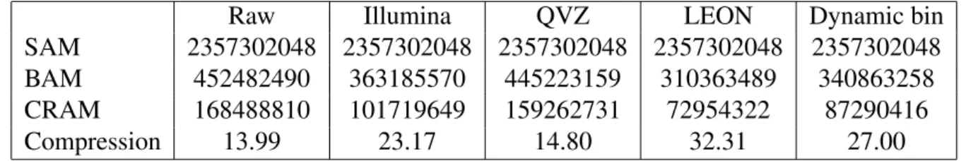
7.1.1 Compression Ratio . . . 44
7.1.2 Variant Calling Performance . . . 46
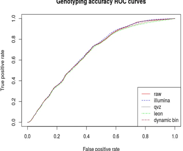
7.1.3 ROC Curve Analysis . . . 47
7.2 Discussion and Analysis . . . 48
8 Conclusions and Future Work 51
Bibliography 53
Appendices 61
A Results of 5x fold coverage experiment 61
B Results of 6x fold coverage experiment 64
List of Figures
2.1 DNA 3D structure. (a) DNA double helix structure. (b) Base pairs formed by
A-T and C-G [4] . . . 5
2.2 Gene structure, [5] . . . 6
3.1 Growth of DNA sequencing [6] . . . 13
3.2 Partial Sam file . . . 17
3.3 Partial Fastq file . . . 18
4.1 Quality values histogram, chromosome 20. Red values are the representatives of each bin. . . 29
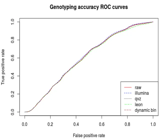
5.1 ROC,chromosome 11 (5x fold coverage). . . 36
5.2 ROC,chromosome 20 (5x fold coverage). . . 37
6.1 ROC,chromosome 11 (6x fold coverage). . . 42
6.2 ROC,chromosome 20 (6x fold coverage). . . 43
7.1 ROC,chromosome 11 (50x fold coverage). . . 48
List of Tables
3.1 SAM format mandatory fields . . . 17 3.2 Q-score Bins for an Optimized 8-level mapping . . . 21 4.1 VCF format specifications . . . 26 4.2 Q-score Bins for dynamic binning, valueci, for a given bin with range[l,r], is
such thatH(ci)≥H(c)∀c∈[l,r]. . . 29 5.1 Chromosome 11 (5x fold coverage), files size(bytes) and compression ratio . 33 5.2 Chromosome 20 (5x fold coverage), files size(bytes) and compression ratio . 33 5.3 Variant calling performance with Illumina ground truth, chromosome 11 (5x
fold coverage). . . 35 5.4 Variant calling performance with Illumina ground truth, chromosome 20 (5x
fold coverage). . . 35 5.5 AUC, Chromosome 11 (5x fold coverage). . . 37 5.6 AUC, Chromosome 20 (5x fold coverage). . . 37 6.1 Chromosome 11(6x fold coverage), files size(bytes) and compression ratio . . 40 6.2 Chromosome 20(6x fold coverage), files size(bytes) and compression ratio . . 40 6.3 Total size after compression, original SAM files size is 66.11GB . . . 40 6.4 Variant calling performance with Illumina ground truth, chromosome 11 (6x
fold coverage). . . 41 6.5 Variant calling performance with Illumina ground truth, chromosome 20 (6x
fold coverage). . . 41 6.6 AUC, Chromosome 11 (6x fold coverage). . . 41 6.7 AUC, Chromosome 20 (6x fold coverage). . . 42 7.1 Chromosome 11 (50x fold coverage), files size(bytes) and compression ratio . 45
List of Tables x
7.2 Chromosome 20 (50x fold coverage), files size(bytes) and compression ratio . 45 7.3 Variant calling performance with Illumina ground truth, chromosome 11 (50x
fold coverage) . . . 46 7.4 Variant calling performance with Illumina ground truth, chromosome 20 (50x
fold coverage). . . 47 7.5 AUC, Chromosome 11 (50x fold coverage). . . 48 7.6 AUC, Chromosome 20 (50x fold coverage). . . 48 7.7 F-score comparison for no quality values. Chromosome 20, ground truth
Chapter 1
Introduction
In recent years the sequencing of human DNA has become a notable field of research from many different areas such as genetics, biology, chemistry, computer science, bioinformatics, etc. The importance that this topic has achieved is due to the broad impact that it has directly on humanity. The influence that it is having on humans goes from understanding DNA, and therefore life and evolution, to health care. In particular, DNA sequencing is being largely used for understanding genetic diseases and their prevention. It also allows the design of specific drugs for specific groups of patients based on their genetic profiles.
In the last twenty years the costs of sequencing human DNA was a barrier for researchers, but since 2015 it became possible to sequence a complete human genome for $1000 [7]. This huge advance in the field implies a large amount of data being generated every day from many big projects around the world such as the 1000 Genomes Project.
It is expected that by the year 2025 [6] two billion human genomes will be sequenced. In general this deluge of data represents a huge challenge from the storage space point of view. Researchers have studied several compression techniques for next-generation output data in an effort to face this problem. The studied approaches for compression of these files vary from general text compression techniques to some more specialized models where the particular properties of DNA strands make the compression more efficient (for example, DNA strands have repetitive content given that the alphabet consists of only 4 letters — A, C, T and G). Nevertheless, there is also much more information reported in the output files than just the DNA sequence (see Section 3.4.1) which makes the compression even more challenging.
Our main target for the study is the quality values reported in FASTQ files, the standard format for storing the output of high-throughput sequencing instruments, as well as SAM (Se-quence Alignment/Map format) files, the standard format for storing read alignments against
1.1. Thesis Structure 2
reference sequences. These quality values report a score per-base associated with the nu-cleotide sequence and can be understood as the probability of an error in the base calling. The alphabet used for these quality scores consists of approximately 40 characters, which repre-sents another barrier for achieving better compression. See Section 3.5 for further information on quality values.
Recently, new lossy models of compression for quality values have been studied [8], [2], [9], [1], [10]. We focus our work in analysing three of them: [2], [1] and [3]. We will also suggest new ideas for adjusting the quality scores, (Section 4.6).
The analysis we will perform is related to the random access CRAM format, see Section 3.4.4. The CRAM format is a new format designed by the European Bioinformatics Insti-tute that compresses SAM/BAM files and achieves 40-50% space saving over the alternative BAM format. The objective of this format is to replace the BAM format and become the stan-dard compression model for sequencing data. We will study the impact of the lossy models mentioned above in this CRAM compression format.
When using lossy compression techniques it is expected that the loss of information should be measured, and the effect of this loss on subsequent tasks performed with the com-pressed data should be also analysed. With the intention of analysing the possible loss of information when adjusting the quality scores, we study the effect that these adjustments will have on the SNP calling performance, which is the process of finding single nucleotide vari-ants in sequencing data. Some recent results [11] suggest that SNP calling performance is not negatively affected, and it can even be boosted when adjusting the quality scores.
1.1
Thesis Structure
This thesis is structured as follows: In Chapter 2 we present the background required to un-derstand this work. Chapter 3 intends to summarize the state of the art related to compression of next-generation output data. Chapter 4 explains all the methodology for the experimen-tal process. Chapter 5, Chapter 6 and Chapter 7 contain the results and the discussion for experiments performed with 5x, 6x and 50x fold coverage data sets, respectively. Chapter 8 concludes this study, and suggests some possible ideas to continue exploring compression of quality values.
Chapter 2
Background
In this chapter we introduce the basic biological concepts required to understand this work. Secondly, we introduce DNA sequencing, its history and the main technologies used for this purpose. Next, we summarize the most important projects related to human genome sequenc-ing around the world and its importance for humanity.
2.1
Basic Biological Concepts
Bioinformatics, according to the Oxford English Dictionary [12], consists of conceptualising biology in terms of molecules and applying informatics techniques to understand and organise the information with these molecules, on a large scale. In other words, this area is about ap-plying knowledge from areas such as applied mathematics, computer science and statistics to analyse physical chemistry of molecules. The recent deluge of biological data, and the prob-lem it represents [13], has made bioinformatics an essential tool for many related applications. In this work we address one of these applications.
2.1.1
Genetics and DNA
Genetics is considered a field of biology for which the principal targets of study are genes. The objective of this area is to understand biological heredity and genetic variation in living organ-isms. The origin of this science dates back to 1865 when Johann Gregor Mendel (1822-1884) published his results about fundamental laws of inheritance that he discovered by working on pea plants for about eight years. The experiments that Mendel performed pointed to the existence of one of the most important biological elements that nowadays we know as genes.
Around the same time Friedrich Miescher in 1869 at the University of T¨ubingen was the first to isolate a substance that he called nucleinand that one hundred years after would be
2.1. Basic Biological Concepts 4
known as DNA. It was in 1953 when James Watson and Francis Crick at the University of Cambridge, based on so many other results and research, discovered and proposed the double helix model of DNA structure. They published their results in the journal Nature [14], [15], and because of this discovery they were awarded the Nobel prize.
After years of research, now we know that DNA, or deoxyribonucleic acid, is a double helix molecule that contains most of the genetic information that makes each individual from each species unique. This structure enables DNA to carry biological information from one generation to the next and it is considered as the blueprint for each living thing. Most DNA is located in the cell nucleus and it is called nuclear DNA. Also, a small portion of DNA can be found in the mitochondria and it is known as mitochondrial DNA or mtDNA. All organisms, in sexual reproduction, inherit half of their nuclear DNA from the male parent and the other half from the female parent. However mitochondrial DNA is inherited in all organisms from the female progenitor.
The two-stranded shape of DNA chemical structure allows biological instructions to be passed along with great precision. Each strand is made up of building blocks known as nu-cleotides and each nucleotide has three parts: a phosphate group, a sugar group and one of four different types of nitrogen bases. The four possible chemical bases are adenine (A), guanine (G), cytosine (C) and thymine (T). The way these bases are ordered dictates the biological instruction contained in the DNA. Another particular property of these bases is that they pair up with each other, A with T and C with G, to form units called base pairs (see Fig 2.1). This property becomes relevant when DNA copies itself during cell division. In this process the double strand structure is split so each one of the strands can be used as template for the pro-duction of the opposite strand. As a result two new double structures are created by pairing up the corresponding bases.
The human genome is built of about 3.2 billion bases considering only one set of chromo-somes. Between each individual, no matter what race, less than 1% of the DNA is different. Research has shown that among these variations of DNA we can find diseases and changes in the cell functions. This is why understanding the human genome is of vital importance.
2.1.2
Genes, Chromosomes and Proteins
The definition ofgenecan be complicated. We simplify the concept by considering a gene as a specific region of DNA that contains instructions usually on how to produce molecules called
2.1. Basic Biological Concepts 5
Figure 2.1:DNA 3D structure. (a) DNA double helix structure. (b) Base pairs formed by A-T and C-G [4]
as per the Oxford English Dictionary [16].
Recent research sets the number of human genes between 20,000 and 25,000 [17] and gene size can vary from a few hundred to more than 2 million bases. Each gene consists of three types of nucleotide sequence (see Fig 2.2):
• Coding regions, called exons, which specify a sequence of amino acids. • Non-coding regions, called introns, which do not specify amino acids.
• Regulatory sequences, which play a role in determining when and where the protein is made as well as how much of the protein is produced.
In human DNA there are always two copies of each gene, one inherited from the mother and the other one from the father. The different forms of the same gene can have differences in their sequence of DNA; these forms are called alleles. The small differences in people’s DNA are what make each person unique in the sense of physical features, although most of the genes are the same in all people.
2.2. DNA Sequencing 6
Figure 2.2:Gene structure, [5]
A long set of nucleotides form genes, and groups of genes are packaged tightly to form important structures in life calledchromosomes. These structures and their DNA are copied as part of the cell cycle and they are passed to daughter cells as part of the process called mitosis and meiosis. Human beings have 23 pairs of chromosomes; 22 pairs of autosomes, which means they look the same in males and females, and one sex pair which differ between males and females.
The process in which genes determine the behaviour of the cell is complex and is con-trolled within each cell. This task consists mainly of two steps calledtranscriptionand trans-lation and is also known as gene expression. This bring us to another important concept, proteins. When a gene is expressed it generates a copy of itself in the form of messenger RNA and then is translated to generate a protein, which is a molecule consisting of long chains of amino acids. Protein structure dictates where it will act and what it will do.
2.2
DNA Sequencing
DNA sequencing is the process in which the precise order of nucleotide bases, adenine, gua-nine, cytosine, and thymine within a DNA molecule, is determined. The importance of this process lies in the fact that the order of the nucleotides determines the instructions for the hereditary properties of life, as well as the biochemical properties. Nowadays knowledge of DNA sequences is indispensable for basic biological research, diagnostics, biotechnology, forensic biology and many other applications.
The first time researchers sequenced DNA molecules was in 1970, by using a series of complicated and time consuming methods. Since then, DNA sequencing methods have evolved and became easier and faster. In 1977 Frederick Sanger introduced thedideoxy
se-2.2. DNA Sequencing 7
quencing method [18], which nowadays is known as Sanger sequencing and until approxi-mately 2005, before the emergence of next-generation sequencing technologies, it was the most used method of DNA sequencing. The Sanger method was the choice of technology to produce the first human genome in 2001. Of course, the time and costs were huge, but the progress in science that this represented was huge as well.
2.2.1
Next-Generation Sequencing
The term next-generation sequencing (NGS) is used to describe a set of modern sequencing technologies such as Illumina (Solexa), Roche 454, Ion Torrent, Oxford Nanopore and others. As a result of these new technologies, DNA sequencing is done more cheaply and quickly than the previous Sanger sequencing technology. Next-generation sequencing is also known ashigh-throughput sequencingand it has revolutionised the study of genomics and molecular biology. NGS is mainly characterized by its improved speed, reduced manpower and reduced cost. All these properties are gained because all these methods are massively parallel, which means that the number of sequence reads for a single experiment is greater than for the experi-ment based on Sanger sequencers. All these DNA sequencing technologies share the property that they cannot read whole genomes in one step. Instead, these machines read small pieces, varying in size from 30 bases to even 30000 bases. These small sequences are calledreads.
2.2.1.1
Illumina (Solexa)
What nowadays we know as Illumina sequencing technologies [19] started in the mid-1990s in the Chemistry Department of Cambridge University with experiments from scientists Shankar Balasubramanian and David Klenerman. The Illumina next-generation sequencing approach differs from the classic Sanger chain-termination method. With these instruments the sequenc-ing is done by synthesis (SBS) technology, tracksequenc-ing the addition of labeled nucleotides as the DNA chain is copied, in a massively parallel fashion. The amount of data that Illumina se-quencing systems can deliver went from 300 kilobases up to one terabase in only a single run, depending on the configuration and instrument used.
As part of the Illumina technologies, there is the most powerful sequencing platform ever created, HiSeq X System, which was released in 2015. The system made it possible to sequence the human genome for only $1000, and is capable of delivering 18,000 of these per year. This sequencing solution is the world’s first to break the thousand dollar human genome barrier.
2.2. DNA Sequencing 8
2.2.1.2
Ion Torrent
This sequencing technology [20] is based on the detection of hydrogen ions that are released during polymerization of DNA. When a nucleotide is incorporated into a DNA strand by a polymerase, a hydrogen ion is released, so if there are two identical bases on the DNA strand the voltage will be double, and the chip will record two identical bases. This detection can be done directly so each nucleotide incorporation is recorded in seconds, because there is no scanning, no cameras and no light like other methods. These technologies were released for the first time in 2010 and up to now they have kept improving, marketing their machines as a rapid, compact and economical sequencer that can be afforded by a large number of laboratories all around the world.
2.2.1.3
Nanopore Technologies
DNA sequencing which works with nanopore-based technology is considered as part of fourth-generation DNA sequencing technologies. It has been under development since 1995 but it was not until February of 2012 that Oxford Nanopore Technologies (ONT) released prelimi-nary experimental results from GridION system [21] using this technology.
A nanopore is a tiny hole with internal diameter at the order of 1 nanometer. In this type of technology the idea is to pass DNA molecules through the nanopore. The scale of the nanopore forces the DNA to pass as a long string, one base at the time. Depending on which base is blocking the nanopore, A, C, T or G, the amount of current needed is different.
2.2.2
DNA Assembly
Given the fact that DNA sequencing machines cannot read the whole genome, the output of this technology is a large set of reads, which are small sub-sequences. The process in which this large set of reads is organized and put back together to re-build the genome is calledDNA assembly. This process has represented a big challenge because of the large amount of data that needs to be processed. There are two main methods of DNA assembly. The first one is
reference alignment consisting of the alignment of all reads against one reference genome. The second one is calledde novo assembly, which does not need a reference genome, making use of the overlaps information contained in the read themselves.
2.3. Human Genome Project 9
2.3
Human Genome Project
After DNA sequencing became widespread since 1977, the idea of large-scale sequencing started to be discussed by human geneticists. It took years for the idea to become an action plan, but finally in 1990 the Human Genome Project (HGP) was announced. The main goal of this project was to complete mapping and understanding of all genes in human beings. The time for doing this was expected to be 15 years.
This project stands as the world’s largest collaborative biological project. At the start it was funded by the Department of Energy and US National Institutes of Health, and later in the UK from the Medical Research Council and Wellcome Trust which helped to run this project on a huge scale, with sequencing centres in France, Germany, China and Japan also joining the big project. The large collaboration around the world made it possible to finish two years before expected. In April 2003, the Human Genome Project was declared complete [22].
The final sequence released by HGP of about 3 billion DNA bases, for the haploid genome, covers about 99% of the human genome for regions that contain genes and it was sequenced to an accuracy of 99.99 percent, which helps to understand better the organization and structure of genes. Besides the human genome, this project included the sequencing of the mouse genome, and the identification of more than 3 million human genetic variations. All sequenced data generated by HGP is available in public databases for all scientists around the world, a fact that has led to an outstanding advance in health science discoveries. The complete human genome sequence started a series of more in-depth comparative studies and generated a large amount of raw data that required specific computing infrastructures, soft-ware implementation and biological data analysis, problems that bioinformatics is trying to solve.
2.3.1
The 1000 Genomes Project
The 1000 Genomes Project was a joint effort among several research groups from the US, UK, China and Germany to produce a catalogue of human genetic variations. This project ran from 2007 to 2015 and its principal goal was to find most genetic variations with frequencies of at least 1% in the populations studied. The large catalogue created has allowed medical researchers to find genetic differences that contribute to rare and common diseases. Locating and analysing these genetic variations leads to discovery of new diagnostic tests and in some cases treatments. The whole project was divided into three phases and respective publications
2.4. Genome Analysis 10
were made public for research purposes: Pilot Analysis [23], Phase 2 Analysis [24] and Phase 3 Analysis [25], [26]. The final version released by the project contains low coverage and exome sequence data for 2,504 individuals from 26 different populations and data for 24 in-dividuals that were sequenced to high coverage for validation purposes. As part of the 1000 Genomes Project the Data Coordination Center (DCC) was set up to manage project-specific data flow, to ensure archival sequence data and to manage community access. This repre-sented a fundamental challenge for bioinformatics considering that as of March 2012 there were more than 260 terabytes of raw data [27].
2.3.2
Platinum Genomes Project
The Platinum Genomes Project is a data set publicly available released by Illumina performed on Illumina HiSeq systems [28]. It has data from the 17 member CEPH pedigree 1463 that was sequenced to 50x depth and one trio sequenced to 200x depth. This project also made public a set of high-confidence variant calls for NA12877 and NA12878 members by taking into account the inheritance constraints in the pedigree and the concordance of variant calls across different methods.
2.4
Genome Analysis
DNA variations are linked to genetic disorders, so they are the target of health researchers. Nowadays, with all of the data obtained from sequencing technologies they are making consid-erable advances and allowing the discovery of treatments and in some cases cures for genetic diseases.
2.4.1
Mutations and Polymorphisms
Mutationis the natural process in which the DNA sequence is changed. More regularly only a single base, A, T, G, C, is substituted for another, but also sometimes a base can be deleted or an extra base can be added. However the cell is able to naturally repair most of these changes and also not all mutations are responsible for something bad or dangerous for the living organism.
Genetic differences that occur in more than 1 percent of the population are called poly-morphisms, and these changes in DNA are common enough to be considered normal variation. Normally these kinds of polymorphisms are the cause for common differences between people such as blood type, complexion, skin color and eye color.
2.4. Genome Analysis 11
Although many polymorphisms in human genomes are not related to a person’s health, some of these variations may influence the risk of developing certain disorders as well as genetic diseases such as cancer among others. What happens is that if a mutation occurs in a functional part of DNA, which is called thecoding area, it may prevent one or more proteins from working properly causing the genetic disorder.
2.4.2
Variant Calling
Variant calling is known as a set of processes for finding variations in data from next-generation sequencing technologies. These computational methods are based on known pop-ulation single nucleotide polymorphisms (SNP). The large amount of data today is making these techniques more challenging and a wide variety of algorithms have been specifically designed.
For understanding how the variant calling algorithms work, first we have to remember how the main NGS technologies work (Section 2.2.1). They generally do sequencing by synthesis. The synthesis process is captured in a series of fluoresce images and base-calling algorithms infer the actual nucleotide information. Then they assign a measure of uncertainty orquality scoreto each base call. Of course base-calling procedures vary depending on the sequencing system. Once having the base-calling and its respective quality score, the process of obtaining a set of genotypes— DNA sequences which determines a specific characteristic (phenotype)— for each individual in a sample is divided into two steps: SNP calling and genotype calling.
SNP calling or variant calling is part of the process that determines where polymorphisms exist or where there is a difference from a reference sequence in at least one of the bases. Genotype calling consists of determining the genotype for each individual which is highly related to the position of a SNP or a variant that has already been called.
Normally the SNP calling process will consist of a series of steps which includes filtering before and after, but the main algorithm is usually a statistical model or some heuristics to predict the likelihood of variation at each locus, based on the quality scores and counts of the aligned reads at that locus.
Chapter 3
Literature Review of Compression for
Sequencing Data
In this chapter we introduce the problem of Big Data related to next-generation sequencing data. We also present an overview of general and particular compression techniques for se-quencing data that already exist. We introduce the quality values, which are the main focus of our research. We summarize the state of the art of lossy compression techniques for quality values and we provide a brief discussion about it.
3.1
Big Data in Genomics
Next-generation sequencing technologies and their continuous improvements have revolution-ized several areas in biology and health sciences by reducing the time and cost required for sequencing. As of 2015 [7] the cost of sequencing the human genome has been reduced to $1000. This fact has led to the generation of a large amount of data, as a typical data file varies from tens to hundreds of gigabytes of disk space. And although, so far, the main successful focus has been investing in data generation [13], the final goal of all this sequencing develop-ment is to be able to analyse and understand DNA, which means that a collateral challenge is not only the storage but the distribution and data analysis as well. For example, the raw data obtained by the 1000 Genomes Project (Section 2.3.1) after six months of activity exceeded the sequence data in NCBI Genbank database accumulated in the preceding 21 years [13].
Big Data in genomics has been compared with three of the largest generators of Big Data: astronomy, YouTube, and Twitter [6], which makes evident the huge challenge that scientists are facing with this issue. For a wider perspective refer to Figure 3.1.
3.2. General Data Compression 13
Figure 3.1:Growth of DNA sequencing [6]
least 2.5 million plant and animal genome sequences, as the result of massive projects around the world [29], [30]. Also, for the same year, they estimate between 1 billion and as many as 2 billion human genomes. Translating all this to disk space, they have determined that until today, even only considering 20 of the largest institutions, the storage required is more than 100 petabytes and they predict that just for human genomes the storage capacity that will be needed in 2025 is as much as 2-40 exabytes.
Considering the challenge of storing such large amounts of data, it is natural to think about data compression. Within the next pages the objective is to show how the Big Data problem in genomics has been tackled, the different techniques that have been used, and all the possibles approaches that still need further research and experiments.
3.2
General Data Compression
In general data compression refers to the set of different techniques for handling huge data of any kind by reducing the space needed to store this data and speed up the data circulation. Strictly speaking, a compression algorithm takes an inputX and generates a representationXc
that requires fewer bits. There is also the inverse process, which operates on the compressed representationXc to generate the reconstruction,Y [31]. Depending on the reconstructionY, data compression schemes can be either alosslesscompression technique ifY is identical to
3.2. General Data Compression 14
X orlossycompression technique ifY is only an approximation forX; the latter implies that the original data cannot be recovered exactly.
3.2.1
Measures of Performance
Evaluation of compression algorithms can be done from many different approaches; it can be evaluated by the relative complexity, the memory required by the algorithm implementa-tion, the speed given by how fast the algorithm performs on a given machine, the amount of compression and how closely the reconstruction resembles the original data.
For measuring the amount of compression the most common technique is called com-pression ratiowhich is simply the ratio of the number of bits required to represent the original data over the number of bits required to represent the data after compression.
In lossy compression, the reconstruction differs from the original data. This difference is calleddistortion. The measure of this distortion is an indicator of the algorithm efficiency. There are many distortion metrics (refer to [31] for more details).
Nowadays data compression is present in almost every application, and is used for text, images, sounds and video. Below we present a broad overview of the most commonly used techniques.
Huffman Coding
Huffman coding is a lossless compression data technique based on Huffman codes developed in 1952 [32], which are a specific type of prefix code.
This algorithm assigns binary codes to symbols of a given alphabet in such a way that the overall number of bits used to encode a typical string formed with those symbols is optimally minimized.
Lempel-Ziv
The Lempel-Ziv algorithm was published for the first time in 1977 [33]. After that, the authors published several variations, all based on the main idea of a sliding window during compres-sion. As result of this algorithm the transmission of the data consists of a set of addresses and the length of the copied segment.
Burrows-Wheeler Transform
Burrows-Wheeler’s Transform [34] is a lossless data compression algorithm, mainly based on block sorting of the input. For each block in the input data, this algorithm applies a reversible
3.3. Sequencing Data Compression 15
transformation, which reorders the data. The idea for reordering is to group characters to-gether. Although the transformation itself does not compress the data, standard compression algorithms can be applied with much more efficient results to the reordered data. The men-tioned efficiency is given because, after the transformation, the probability of finding two instances of the same character close to each other has been substantially increased and this specific property is exploited by a combination of other common algorithms such as move-to-front, Huffman and arithmetic coding.
Arithmetic Coding
The arithmetic coding algorithm for data compression was popularized in 1987 [35] and can be used in lossless and lossy compression models.
The important process of this algorithm consists of the conversion of input data consisting of a set of symbols into a floating-point number in the interval[0,1). The conversion relies on a model to characterize each symbol during the time of processing.
Golomb Coding
In 1960 Solomon W. Golomb [36] invented the data compression codes used for lossless data compression. This algorithm is based on a model of the probability of the values: one natural number is assigned to each value according to its probability, with small values more likely than big ones. One important parameter for the code is the divisor which captures the relationship between size and probability.
3.3
Sequencing Data Compression
Compression of DNA sequencing data started even before the big data revolution that whole human genome sequencing and NGS technologies brought in latter years. The first approaches for sequencing data were based on text compression techniques which were adapted to exploit obvious properties of DNA sequences such as the 4-letter alphabet, regularities and presence of palindromes [37]. All these previous techniques were characterized by using a combina-tion of two different methods: firstly, substitucombina-tional or diccombina-tionary based, where most repetitive sub-sequences are identified and encoded with a representation of smaller size, and secondly, statistical based methods, in which a prediction model is established which assigns probabili-ties to each base based on the data and then uses an encoding scheme that will perform more efficiently based on the probability distribution.
3.4. Next-Generation Sequencing Data Compression 16
Among the most relevant within this path of research we have XM [38] which trains a second-order Markov model on the full data and uses arithmetic encoding[35] relying on the calculated probabilities, CTW-LZ [39] which uses the context tree weighting prediction model and Lempel-Ziv [33] algorithms for compression. BioCompress [40] and BioCompress2 [41] use both Lempel-Ziv and arithmetic encoding, and there are others following the same idea such as GenCompress, [42] DNACompress [43] and GeNML [44].
3.4
Next-Generation Sequencing Data Compression
With all the advances from NGS technologies new challenges also emerged for compression of its output data because these technologies, along with the sequence or read itself, also report additional metadata needed for downstream DNA analysis. This metadata includes a larger alphabet than the 4-letter alphabet, the one that had been considered for sequencing data compression until that time. Therefore new research and techniques for sequencing data were necessary. We will give an overview of the research that has been developed. First we introduce the data formats which are the target for compression in all these problems.
3.4.1
Data formats
3.4.1.1
Sequence Alignment/Map format (SAM)
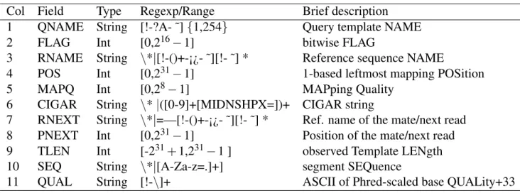
The Sequence Alignment/Map (SAM) [45] format is a generic alignment format for storing read alignments against reference sequences. It has been developed with the main purpose of allowing DNA analysis and the exchange of information from various sequencing platforms. This format consists of an optional header and then each line represents the linear alignment of one read. Each line has 11 mandatory fields described in Table 3.1. For an example of this file see Figure 3.2. There is also BAM format which is the binary version of a SAM file and is designed to compress reasonably well. These two formats are nowadays the industry standards for reporting alignment/mapping information. Also all the important tools for analysis of high-throughput sequencing data require these formats as the input. Examples of these tools are GATK [46], Samtools [47] and FreeBayes [48].
3.4.1.2
FASTQ Format
FASTQ format [49] was originally developed at the Wellcome Trust Sanger Institute and it has become the standard format for storing the output of high-throughput sequencing instruments. This format is used to store the nucleotides sequence and its corresponding quality scores,
3.4. Next-Generation Sequencing Data Compression 17
Col Field Type Regexp/Range Brief description
1 QNAME String [!-?A- ˜]{1,254} Query template NAME
2 FLAG Int [0,216−1] bitwise FLAG
3 RNAME String \*|[!-()+-¡¿- ˜][!- ˜] * Reference sequence NAME
4 POS Int [0,231−1] 1-based leftmost mapping POSition
5 MAPQ Int [0,28−1] MAPping Quality
6 CIGAR String \*|([0-9]+[MIDNSHPX=])+ CIGAR string
7 RNEXT String \*|=—[!-()+-¡¿- ˜][!- ˜] * Ref. name of the mate/next read
8 PNEXT Int [0,231−1] Position of the mate/next read
9 TLEN Int [-231+1,231−1 ] observed Template LENgth
10 SEQ String \*|[A-Za-z=.]+] segment SEQuence
11 QUAL String [!-\]+ ASCII of Phred-scaled base QUALity+33
Table 3.1: SAM format mandatory fields
Figure 3.2:Partial Sam file
each of them encoded with a single ASCII character. Each line in the file uses four lines per sequence, containing the read id (always starts with ’@’), the sequence, an optional description or default ’+’ sign and a last line for the quality values. See Fig 3.3 for a better idea of how a FASTQ file looks.
3.4.2
Reference-based Compression
Considering that DNA strings contain only four possible letters, A, C, G and T, it is expected that there are many repetitions between the sequences, and this property has been broadly ex-ploited for compression techniques of DNA sequencing. The methods grouped as reference-basedfollow two essential steps. First they choose a reference sequence and then only encode
3.4. Next-Generation Sequencing Data Compression 18
Figure 3.3:Partial Fastq file
the differences between the sequence to be compressed and the reference. For a good perfor-mance of this method the choice of the reference sequence is important. There are some cases in which instead of one reference a set of possible references is allowed [50], [51], [52]. As another example, in [53] the genome is divided into blocks and for each position the longest matching block is compressed. Also, in [54], only differences between similar or overlapping reads are encoded. Also, Deorowicz and Grabowski [52] propose a technique which has a reference genome in addition to other short sequences taken from the data to be compressed. There are other approaches focused only on output of NGS technologies, namely SAM and FASTQ formats. For FASTQ format there is Fastqz [55] which encodes the DNA alphabet and uses Lempel-Ziv encoding for matched and mismatched positions against a reference. Gencompress [56], also reference-based, calculates statistics on the mismatches and performs the encoding based on these statistics. For SAM format mzip [57] uses Huffman coding for compressing only position and read length; Samcomp [55] and NGC [58], SlimGene [59] and Quip [60] are also in this category.
3.4.3
Reference-free Read Compression
De novo or reference-free compression is performed without an external reference genome. Instead, this kind of method exploits similarities between reads themselves [55], [61], [62], [63], [64], [65]. Most commonly this technique will use a context-model to predict the bases and then use an arithmetic encoder or they will re-order reads to maximize similarities for consecutive reads allowing a better compression with standard methods. FQZCOMP [55] and DSRC [62] are examples of the context-model compressors; PATHENC [66] is also of
3.5. Quality Values 19
this type complemented with arithmetic encoding. According to [2] read re-ordering methods are the ones that achieve a better compression ratio. Compressors of this type are BEETL [64] which uses Burrows-Wheeler transform, ORCOM [63], MINCE [65] and more recently, LEON [2], which proposes a method based on a probabilistic de Bruijn graph stored in a Bloom filter [67].
3.4.4
Random Access and CRAM Format
Although compression is mainly focused on solving the problem of storage and distribution of Big Data, it is also possible to make more practical the step of analysing the data, by applying particular compression techniques for specific files. This type of compression allows us to access part of the file, from its compressed version, without going through the entire decompression process. For achieving random access compression generally the input is split into blocks and even different compression algorithms can be applied to different blocks within the same file.
Today, BAM format[45] is the standard compression model with random access property achieving compressions of 50-80% of their original SAM file and allowing an accessible and practical analysis of sequencing data using the compressed file. Although it is a huge success and it is supported by most sequencing data analysis tools, the compression ratio achieved is not sustainable in the long run as sequencing data is growing at a big rate. Because of this, researchers have explored new options, and as one of the best results CRAM framework technology has been developed. CRAM [68], based on the work of Fritz et al. [57], is a new format designed by the European Bioinformatics Institute that compresses SAM/BAM files and achieves 40-50% space saving over the alternative BAM format. The objective of this format is to replace the BAM format and become the standard compression model for sequencing data. In recent years it has gained huge popularity in the area and its popularity is expected to grow even more. By now it is supported for the main tools for analysis of sequencing data and also big initiatives such as the 1000 genomes project have their data available for public use stored in this format.
3.5
Quality Values
The base calling process performed for NGS technologies to determine the bases of a DNA string is prone to a different type of error. In order to report the probability of base calling mistakes, sequencers generate a quality score for each nucleotide in the read.
3.6. Lossy compression for sequencing data 20
A quality score indicates the level of confidence of a particular read base and is repre-sented as the probability of the base being correctly determined during sequencing. The higher the score, the lower the probability that the base at that position has been incorrectly called. It is generally computed usingPhred score[69] which is the numberQ=−10log10P, whereP
is the estimated probability of the corresponding nucleotide being incorrect, calculated by spe-cific software running in the sequencing machine. Usually the quality values are represented in a file with a printable ASCII alphabet [33:73] or [64:104], with each value corresponding toQ+33 orQ+64, respectively. The importance of maintaining quality scores as part of the data relies on the fact that they are directly used in next-generation sequencing analysis, such as Single Nucleotide Polymorphism(SNP) detection [70]. Quality scores comprise a signif-icant percentage of sequencing data and they became a bottle neck for compression because the alphabet required to represent all quality values is larger —about 40 characters— than the one required for the read sequence. Therefore compression algorithms designed for the sequence itself will not perform quite as well when applied to quality values. For this purpose, specific algorithms must be provided taking into account particular properties and information that quality scores have themselves.
3.6
Lossy compression for sequencing data
As we mentioned before, there are lossless and lossy techniques for data compression. Nev-ertheless lossy techniques are not allowed for DNA sequences due to the fact that losing or changing one single nucleotide represents a big impact on the possible encoded protein. How-ever researchers have applied this technique not to the DNA sequence itself but to the quality values reported for each base, which represents almost half of the total data in the output file. There are in the literature several techniques trying to solve the problem of quality values compression by using lossy techniques [8],[2],[9], [1],[10].
When lossy compression techniques are applied to any type of data, the natural path to follow is to measure the loss of data and in good cases the missed data should not affect or mislead any other possible output derived from the compressed data. Any lossy technique in this field should show that downstream analysis, SNP calling, is not affected. A good starting point for this type of analysis is [10], which suggests that quality values data is noisy data, and which presents an analysis where losing precision in quality score was actually beneficial for SNP calling.
3.6. Lossy compression for sequencing data 21
Quality Score Bins Mapped Quality score
N(no call) N(no call)
2-9 6 10-19 15 20-24 22 25-29 27 30-34 33 35-39 37 ≥40 40
Table 3.2:Q-score Bins for an Optimized 8-level mapping
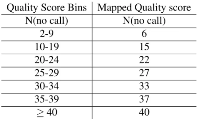
C´anovaset al. [8] proposed a lossy technique where the quality values were separated into blocks of variable size, each block with only one representative value which depends on the distortion measure selected for the user from a set of possible measures. Concurrently, Illumina [3] suggested what today is known as illumina binning, in which the resolution of quality scores was reduced by employing a quality scoring scheme with only eight levels of quality or less. Their complete binning is presented in Table 3.2.
The same year, Ochoa et al. [10] presented QualComp, a lossy compressor for quality scores based on rate distortion. In this framework the user is allowed to specify the number of bits per quality score prior to compression. This compressor works with FASTQ files and performs in clustering model.
More recently, researchers from Stanford University published a new approach,Quality Values ZipQVZ [1], based on the same ideas as [10]. In this work the quality score sequence is modelled as a Markov chain of order one. Then empirical transition probabilities are computed from the data, a collection of Lloyd-Max quantizers are constructed (one for each possible base in each position) and finally an arithmetic encoder is run over the result.
Benoitet al. [2] proposed a reference-free compression model for sequencing data; they present the model for reads compression and they use the same construction for implementa-tion of lossy compression for quality values. Their process consists of building a de Bruijn Graph of the most recurrentk-mersin the sequences, with each read encoded as a path in this graph. For quality score compression, they truncate all quality values above a given threshold. Also all positions covered by at least a certain number of recurrentk-mersare replaced by one representative value, with this number computed based on the quality value so that the lower the quality the higher the number of coveringk-mersis required.
3.7. Comparison and Discussion 22
3.7
Comparison and Discussion
Lossy compression techniques for quality values is a very recently explored area, with the first ideas presented in 2011. During our research on the state of the art of quality values compression we realized that the main ideas have evolved so that nowadays they are used in more new discoveries. We have analyzed results mainly from the most recent research [2], [1], [10], as we consider it contains also previous research and the comparison they presented suggests more worthy results to consider when it comes to studying this topic.
When comparing two or more lossy compression techniques, there is not a general rule about how to proceed. There are many factors involved in the result and there is always a trade off between compression ratio and any other measure, that can be distortion rate, impact on downstream analysis, speed or memory requirements. For measuring distortion rate many different metrics are used as can be appreciated in [8], [1] and [10]. For rating impact on downstream analysis —SNP calling— the scores are normally presented using F-score which considers both precision and recall measures. This measures are defined in Section 4.5.
Qualcomp [10] focusses its comparisons and performance measurement on rate distortion metric, specifically working with mean square error. Qualcomp compression allows the user to specify the number of bits per quality score, so they present the relationship between number of bits per quality score and mean square error.
For downstream analysis they study SNP calling but we note that they consider as ground truth the data resulting from variant calling performed with the original quality values. They also accept that the running time for their algorithm is longer than the ones they are comparing against[61], [55]. Nevertheless they achieve better compression ratio minimizing mean square error and only a little is compromised in SNP calling.
C´anovaset. al[8] presented their work and compared it against Qualcomp. In this case they used several fidelity measures and showed that their method outperformed Qualcomp when considering Max : Min Distanceas the measure. They also based their SNP analysis considering variant calling with original quality values as benchmark. They did not report data for running time and memory storage.
The next year, in 2015, Malysa et al. [1] released QVZ for quality values compres-sion. They also measured their performance with distortion rate metrics, including mean square error, average L1, where d(x,y) =|x−y| and average Lorentzian where d(x+y) =
3.8. Objective of this work 23
of C´anovaset al. for all three choices of distortion metric. Also a few months later they pub-lished an exhaustive analysis on the effect of lossy compression of quality values using QVZ on variant calling [71]. This analysis included SNP calling compared against two different sets for benchmark recently released, one by GIAB (Genome in a Bottle) and adapted by the National Institute of Standardizations and Technology (NIST) and the other one by Illumina as part of the Platinum Genomes project. For their comparisons, along with the previously mentioned algorithms, they also included the Illumnina binning method, see Table 3.2. The main contribution of their work is not only the reduction of storage space but also their proof that SNP calling is not affected. Moreover, they confirm with their experiments that smoothing quality values can improve it.
Benoitet al. [2] presented a model for sequencing data. Their algorithm was based on a probabilistic de Bruijn graph that was designed originally for compression of the sequence (read). Once they built the graph, they also used it to perform a lossy transformation of the quality values. We have to consider this for comparisons because the probabilistic de Bruijn graph has high memory requirements. For comparison against other algorithms they selected models with option to compress with lossy techniques as well [55], [61], [65]. Their new algorithm performed better when considering compression ratio, compression time and decompression time. They also presented SNP calling analysis considering as bench mark set the variants provided by the 1000 genomes project and also showed that lossy techniques on quality values can improve SNP calling.
3.8
Objective of this work
In this work we address the compression of SAM files which is the standard output file for DNA alignment. We specifically study lossy compression techniques used for quality values reported in the SAM. We selected three of the most promising lossy techniques: QVZ [1], LEON [2], Illumina binning [3], and we also introduce a new lossy model, dynamic binning technique. The objective of this study is to analyse and discuss how each of these lossy techniques will perform when using the CRAM compression format for SAM files. Because we are analysing lossy techniques for quality values we also want to provide evidence that these kinds of methods will not impact negatively in the SNP calling process. For such purpose we provide an analysis of SNP calling performance.
Chapter 4
Methodology
In this chapter we present all toolkits and software used for our research. We introduce the data sets for the experiments as well as the sets used as ground truth for evaluation of SNP calling. We also present the metrics for SNP calling performance. And we explain the experimental process followed in our work.
4.1
Toolkits
4.1.1
GATK
GATK stands for Genome Analysis Toolkit [46]. It was developed by the Data Science and Data Engineering group at the Broad Institute. This toolkit is a collection of command-line tools for analyzing high-throughput sequencing data in formats such as SAM/BAM/CRAM (see Section 3.4.1) and VCF (see Section 4.2) with a primary focus on variant discovery and genotyping.
When using GATK for variant calling we follow GATK Best Practices [72], [73], which is the recommended workflow for variant discovery analysis with GATK. This process intends to maximize the technical correctness of the data. The first steps start from the raw reads indicating how to do the mapping to a reference genome, marking duplicates with Picard tools (see subsection 4.1.4) and performing a base quality score recalibration. Once the data has been pre-processed it is ready to continue with the variant discovery process. In this second part the process considers the fact that some of the variation might be caused by mapping and sequencing artifacts. Finding a good trade-off between sensitivity (minimizing false negatives) and specificity (minimizing false positives) can be very difficult, and can also be dependant on the project, Instead, the process maximize sensitivity but they also report a variant quality score recalibration (VQSR) which further allows the user to customize specificity for each
4.2. VCF Format 25
project.
4.1.2
Samtools
Samtools [47] is a suite of programs for interacting with high-throughput sequencing data in formats such as SAM/BAM/CRAM. Samtools makes it possible to work directly with a compressed BAM/CRAM file, without having to uncompress the whole file. We also use this toolkit for making SNP calling throughmpileupcommand, which calculates genotype likeli-hoods supported by the aligned reads and does the SNP calling based on those likelilikeli-hoods.
Bcftools is another module included in samtools and we use it for handling VCF files, see Section 4.2.
4.1.3
HTSlib
HTSlib is a C-library for manipulating file formats such as SAM, CRAM and VCF. It is used for studying high-throughput sequencing data and is the core library used by samtools.
4.1.4
Picard
Picard [74], also created by Broad Institute developers, is an open source under MIT license set of command line tools for manipulating high-throughput sequencing data. We specifically use this toolkit for marking duplicate reads as part of the GATK Best Practices.
4.1.5
BWA
Burrows-Wheeler Aligner (BWA) [75] is a software package for mapping low-divergent se-quences against a large reference genome, such as the human genome. When performing alignments with this software, we considered the reference genome GRCh37 called hu-man g1k v37.fasta available at [76], which corresponds to the reference genome used in phase1 and phase3 of 1000 Genomes Project.
4.2
VCF Format
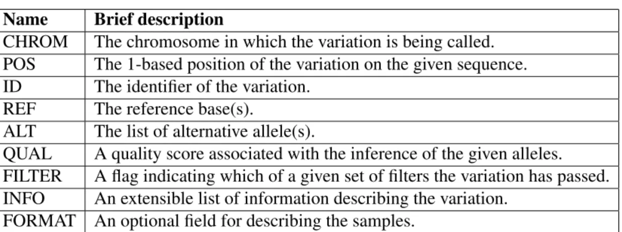
The Variant Call Format (VCF) [77] is a text file format for storing gene sequence variations. It consists of a couple of lines for meta-information, a header line, and then is followed by a number of lines that each contains information about a variation in the genome. It is also possible to store genotype information on samples for each position in this format. There are eight mandatory fields for each reported variation and they have to follow a specific order as well, see Table 4.1 for further explanation. A VCF file will be the output of variant calling
4.3. Datasets For SNP Calling 26
Name Brief description
CHROM The chromosome in which the variation is being called. POS The 1-based position of the variation on the given sequence. ID The identifier of the variation.
REF The reference base(s).
ALT The list of alternative allele(s).
QUAL A quality score associated with the inference of the given alleles. FILTER A flag indicating which of a given set of filters the variation has passed. INFO An extensible list of information describing the variation.
FORMAT An optional field for describing the samples. Table 4.1: VCF format specifications
performed with either GATK tools or Samtools.
4.3
Datasets For SNP Calling
For analyzing the impact of lossy compression models for the quality values we use datasets from 1000 Genomes project. All datasets correspond to the Homo Sapiens individual NA12878. This individual is the daughter in one of the trios sequenced from Utah residents of northern and western European ancestry (CEU). Specifically we use the low coverage ment (6x) to perform the experiments with the whole genome (22 chromosomes). This align-ment is provided by 1000 Genomes project and available at their public repository [78]. We also extracted chromosome 11 and 20 from the whole genome with high coverage alignment (50x), available at the same repository. And finally, for a complete process experiment, we consider the read dataset SRR622461 for the same individual (NA12878) with 5x coverage; for this raw dataset we performed the alignment with bwa software [75]. We have selected individual NA12878 because it is the only one for which a well analysed ground truth set of variants has been developed and has been publicly released.
4.4
Quality Benchmark for SNP Calling
For having a measure of how lossy models can affect SNP calling, we first need to set the baseline that will serve as a reference when comparing the performance of lossless compres-sion against the different lossy comprescompres-sion models. For this purpose we use twoground truth
sets of variants that have been developed and refined specifically for individual NA12878. The first set of variants that we consider as ground truth was released by the Genome in a Bottle consortium (GIAB) [79] and it has been adapted by the National Institute of Standardizations
4.5. SNP Calling Performance Metrics 27
and Technology (NIST). In their work [79] they integrated and arbitrated between 14 data sets from five sequencing technologies, seven read mappers and three different variant callers resulting in a set of variants which allows high-confidence SNP calling without depending on specific caller or sequencing technologies. The second gold standard we used is the one released by Illumina as part of the Platinum Genomes project.
4.5
SNP Calling Performance Metrics
When comparing two different lossy models for quality values, we will evaluate how each one of them affects SNP calling. For this purpose, we consider this problem as a binary classifier for the variants. This will allow us to divide each variant in the resulting VCF file, as True Positive (TP) when the same variant is also part of the ground truth and False Positive (FP) when the variant in the resulting VCF file can not be found in the ground truth. We also examine False Negatives (FN) which are the variants in the ground truth that cannot be found in the resulting VCF file.
By considering this segregation we can do the performance evaluation with typical met-rics such as sensitivity, precision and F-score.
1. Sensitivity, also known as the true positive rate or recall, measures the proportion of correctly identified positives and is given by the expression:
Sensitivity= T P
T P+FN. (4.1)
2. Precision, also known a positive predictive value, measures the proportion of identified positives that are true and is given by the expression:
Precision= T P
T P+FP. (4.2)
3. F-scoreis a metric for accuracy in binary classification. This score considers both pre-cisionandsensitivityby computing the harmonic mean of them. It can be interpreted as a weighted average and is computed as:
F−score=2×Sensitivity×Precision
4.6. Dynamic Binning 28
When analyzing results given by these metrics we interpret them considering that a per-fectSensitivity score of 1.0 indicates that all variants from the ground truth were correctly identified, although it does not indicate how many irrelevant variants were also called as pos-itive. On the other hand, a totalPrecision score of 1.0 means that all obtained variants are relevant but indicates nothing about the total of possible positive variants. Generally there is always a trade-off between these two metrics and depending on the case one could prefer to increase one of them by causing a decrease in the other one. Because of this, F-score, which combines both metrics, will give us a better overall evaluation.
4.5.1
ROC Curve
Receiver Operating Characteristic (ROC) curve is used to visualize the performance of a bi-nary classifier while varying a certain discrimination threshold. This curve is the result of plotting the true positive rate (TPR) against the false positive rate (FPR) with different thresh-olds.
When evaluating variant calling performance with metrics sensitivity, precision and F-score, we considered all variants in an output VCF file to be correct. With this second ap-proach, using ROC as metric, we vary the quality threshold and consider variants in an output VCF file to be correct only if they are above the threshold.
This metric, in this specific problem of variant calling performance, was introduced in the work of William et al. [11]. As in their original work, we follow their design and when comparing different sets of variants we take the union of them as the domain. This rescaling is done with the purpose of addressing the fact that the true negative rate of correctly called variants will be so much larger, as most of the genome will not be variant, and so could cause misleading results. The implication of performing this rescaling is that ROC curves between different plots are not comparable as they will have different domains.
For our analysis we also look at the AUC, area under the curve, which indicates the probability that the binary classifier will rank a random positive case higher than a random negative case. For the AUC, the closer to 1 the better.
For plotting ROC curve and computing AUC, we use ROCR package [80].
4.6
Dynamic Binning
In order to explore new ideas for reducing the alphabet used for quality values, we developed a dynamic binning. As in Illumina binning, this method splits the alphabet into bins. But in
4.7. Experiments Process 29
Quality Score Bins Mapped Quality score
1-10 c1
11-20 c2
21-30 c3
31-40 c4
41-256 c5
Table 4.2:Q-score Bins for dynamic binning, value ci, for a given bin with range[l,r], is such that
H(ci)≥H(c)∀c∈[l,r].
this case it will have 5 bins and the value representing each bin will be the one with the largest number of occurrences belonging to that bin. We apply this method block-wise, which means that the whole file will be split into blocks and for each block the 5-binning will be different depending on its histogram. In our experiment we considered blocks of 1000 reads each, an empirically selected parameter.
For a given block, letHdenote the histogram of the quality values, i.e. for any character
cin that block,H(c)is the number of occurrences of cin the block. The 5-binning for each block is performed according to Table 4.2 where each representative valueci, for a given bin with range[l,r], is such thatH(ci)≥H(c)∀c∈[l,r].
In Figure 4.1 we show an example of a histogram for chromosome 20, 5x coverage, with representative values coloured in red for each bin.
Figure 4.1:Quality values histogram, chromosome 20. Red values are the representatives of each bin.
4.7
Experiments Process
Our purpose with these experiments is to study how we can improve CRAM compression by modifying quality values with four different techniques: QVZ [1], LEON [2], dynamic binning and Illumina binning [3] and also analyze how the lossy models impact on SNP calling.
4.7. Experiments Process 30
In order to perform CRAM compression we need as input a SAM file with the quality val-ues modified by each of the techniqval-ues to analyze. The general work flow of the experiments can be split into the following steps:
1. The very first step is the alignment of the reads to a reference genome. In this case we use BWA MEM command from BWA software and as for the reference genome we work with genome GRCh37. The output of this alignment will be a SAM file that, from now on, we will refer to as the originalSAM and the quality values in it will be the
originalorrawquality scores, as they are the ones provided for the sequencer, in this case, Ilumina technologies.
2. In the second step we create a SAM file for each one of the lossy models that we are analyzing, in which these new files will have the quality scores updated according to each model. Then we convert each SAM file to CRAM format using samtools in order to compare theircompression ratio.
• ForIllumina binningthe process is straight forward and we only modify the code inhtslibso when converting the BAM file to a CRAM file it will apply the corre-sponding transformation to each quality value according to Table 3.2.
• For applying LEON transformation, their software requires a FASTQ file. In this case we create a temporal FASTQ file with the reads and quality values extracted from the originalSAM. We run LEON algorithm with this created file, then we decompress their output and create the new SAM file with the modified quality values.
• On the other hand, the input for QVZ algorithm is only a file with the quality scores, with one read per line. This file is created directly by extracting the quality values from the originalSAM file. Again, once the quality values are processed we decompress the output and create a SAM file with the new quality scores. • As for dynamic binning, we read the file twice. In the first round we compute the
histogram for each block and we create a dictionary of the representative values for each bin corresponding to each block. In the second round we only apply the transformation to the quality values according to the dictionary created in the first round.
4.7. Experiments Process 31
3. Other than only comparing thecompression ratio, we also intend to compare how each of the techniques impact on SNP calling performance. In this step, we follow Best Practices[72], [73] to improve the data.
4. Lastly, we perform the variant calling with two different software tools and compare each one of the lossy models with the mentioned metrics, sensitivity, precision and F-score:
• From Samtools we usesamtools mpileuppipeline.
![Figure 2.1: DNA 3D structure. (a) DNA double helix structure. (b) Base pairs formed by A-T and C-G [4]](https://thumb-us.123doks.com/thumbv2/123dok_us/1356127.2681426/15.892.313.629.143.596/figure-structure-double-helix-structure-base-pairs-formed.webp)
![Figure 2.2: Gene structure, [5]](https://thumb-us.123doks.com/thumbv2/123dok_us/1356127.2681426/16.892.192.747.153.320/figure-gene-structure.webp)
![Figure 3.1: Growth of DNA sequencing [6]](https://thumb-us.123doks.com/thumbv2/123dok_us/1356127.2681426/23.892.138.806.145.527/figure-growth-of-dna-sequencing.webp)
![Table 4.2: Q-score Bins for dynamic binning, value c i , for a given bin with range [l, r], is such that H(c i ) ≥ H(c)∀c ∈ [l, r].](https://thumb-us.123doks.com/thumbv2/123dok_us/1356127.2681426/39.892.302.637.139.261/table-score-bins-dynamic-binning-value-given-range.webp)