World Bank Independence: A Model and Statistical Analysis of U.S. Influence

Full text

(1)World Bank Independence: A Model and Statistical Analysis of U.S. Influence. Robert K. Fleck Department of Agricultural Economics and Economics Montana State University. Christopher Kilby* Department of Economics Vassar College. Vassar College Economics Working Paper #53 June 30, 2005. Abstract: This paper develops a model to test whether World Bank lending caters to U.S. interests. We use country-level panel data to examine the geographic distribution of World Bank lending to 110 countries from 1968 to 2002. After controlling for country characteristics expected to influence the distribution of lending in a manner consistent with the World Bank’s charter and stated allocation mechanisms, we introduce variables reflecting U.S. interests. The empirical results are consistent with a significant U.S. influence, but one which varies across presidential administrations. These findings have important implications because donor influence may reduce the credibility, and hence the development effectiveness, of multilateral aid organizations. Key Words: World Bank, United States, Multilateral Aid JEL Classifications: F35, O19 *. Corresponding author: [email protected]. We gratefully acknowledge helpful comments from two anonymous referees, Margaret McMillan, and participants at the Northeast Universities Development Consortium Conference, the Western Economic Association Conference, the Hamburg Institute of International Economics Conference on the Political Economy of Aid, and the Tri-College summer seminar series at Swarthmore College..

(2) 1. Introduction In recent years, scholars, activists, and the news media have criticized the institutions that distribute foreign aid, charging that donors–most notably the United States–compromise the effectiveness of international aid agencies by pressuring them to deviate from the objectives set out in their charters (The Economist, 2001). One important question raised by these charges is the extent to which multilateral aid allocations respond to donor preferences. This paper examines whether the geographic distribution of World Bank lending reflects U.S. interests. The U.S. is the most influential donor member of the World Bank, a position maintained by the financial structure of the institution, the location of the World Bank in Washington, DC, and the traditional nomination of the World Bank president by the United States. Catherine Gwin (1997) argues that the U.S. has been able to influence World Bank policy when significant U.S. interests are at stake (for example, limiting unfriendly governments’ access to loans). Other researchers and activists claim that the “Washington Consensus” of neo-liberal policies promoted by the World Bank in its policy advice and structural adjustment programs furthers the U.S. agenda. This critique in effect views the World Bank as a thinly disguised tool of the United States government. The World Bank itself maintains that, true to its charter, it is an independent, apolitical, multilateral institution in which all decisions are guided by economic analysis and the best interests of the citizens of borrowing member nations. Perhaps the most basic element of independence for an international aid agency is that its funding allocation decisions depend on equity and efficiency criteria rather than directly reflecting the interests of donor countries. We examine this aspect of World Bank operations, developing a theoretical model which we test with country-level panel data on the geographic distribution of World Bank Group lending from 1968 to 2002. In this framework, independence from the U.S..

(3) should yield a geographic distribution of loans that depends on country characteristics such as population, GDP per capita, and the quality of the policy environment. Controlling for these factors, measures of U.S. interests should be unrelated to the allocation of funds. If the World Bank does respond to pressure from the U.S. in allocating funds, measures of U.S. interests will likely explain some of the cross-recipient and inter-temporal variation in World Bank lending. The paper’s theoretical model of donor-agency interaction develops this insight. The model considers the case of two aid recipients that are identical except that one is favored by the donor. The agency (e.g., the World Bank) prefers a higher budget equally distributed between the recipients, while the donor (e.g., the U.S.) has an ideal budget level and prefers an unequal distribution with the larger share allocated to its favored recipient. Although the agency could adhere to an equal allocation, donor contributions increase if the agency allocates a larger share to the donor’s favored recipient.1 The model predicts that: 1) the allocation process will be biased (relative to equal distribution) in the direction favored by the donor; 2) the allocation bias will be larger when the donor bias is larger; and 3) the allocation will be closer to the donor ideal when donor bargaining power increases (as may happen, for example, during triennial IDA replenishment negotiations). To measure U.S. interests, the empirical analysis uses several variables based on U.S. bilateral aid allocation, U.S. trade statistics, and commercial financial flows. The empirical results are consistent with a significant U.S. influence, but one which varies across presidential administrations. These findings have important implications for the development effectiveness of aid because donor influence may reduce the credibility, and hence the effectiveness, of multilateral aid organizations.2 The literature on aid effectiveness has typically found multilateral aid to be superior to bilateral aid in many “quality” dimensions–all of which depend on the independence of 2.

(4) the multilateral aid institution. Even self-interested donors should balance the short run benefits from controlling a multilateral agency against the long run reduced usefulness of the agency as its credibility is undermined. The impact of donor influence in multilaterals has an important role to play as the ongoing debate over good policies and aid effectiveness continues to shape the aid allocation process (Burnside and Dollar, 2000; Easterly et al., 2004; Klitgaard et al., 2005). 2. Aid Allocation and World Bank/U.S. Relations This paper bridges two distinct branches of the foreign aid literature, one on the allocation of aid and the other on the influence of donors over multilateral aid agencies. The aid allocation literature is primarily empirical, drawing on data collected by the OECD’s Development Assistance Committee and, in some cases, individual donor agencies. The literature on donor influence is based largely on institutional analysis with supporting case studies. The empirical aid allocation literature spans more than thirty years and explores a variety of questions. One major thread examines donor allocation data in an effort to uncover the motives for giving aid.3 Another approach takes the recipient perspective and focuses on allocation outcomes in terms of donor concentration and aid intensity (O’Connell and Soludo, 2001). This work on aid allocation is important for studies of the effect of aid on growth: it provides insight into how the criteria for allocation influence the effectiveness of aid, and it assists in addressing endogeneity problems in aid and growth regressions (Alesina and Weder, 2002; Boone, 1996; Burnside and Dollar, 2000; Mosley,1987). Aid allocation data reveal the “quality” of aid and the degree to which donors achieve target levels of funding.4 Much of the literature focuses on bilateral aid, but some studies cover multilateral organizations.5 Many studies have examined U.S. bilateral aid.6 Although the U.S. provides a relatively large share of bilateral aid funds (the U.S. was the largest donor until 1989 and has been periodically 3.

(5) since then), the quality of U.S. aid has been widely criticized. A substantial literature argues that U.S. aid allocation is not conducive to promoting development (McGillivray, 1989; Zimmerman, 1993) and is characterized by a bias toward middle income countries (Clark 1992). Numerous studies find U.S. bilateral aid allocation to be motivated primarily by geopolitics (especially during the Cold War era), secondarily by commercial interests, and, to a lesser extent, by humanitarian concerns.7 There is an ongoing debate over the influence of recipient countries’ human rights records on U.S. bilateral aid, with much of the analysis comparing allocation patterns across different presidential administrations.8 Studies of U.S. food aid reveal that these programs serve a variety of objectives including humanitarian concerns, geopolitical interests, and the disposal of agricultural surplus (Ball and Johnson, 1996; Eggleston, 1987; Shapouri and Missiaen, 1990). Cold War geopolitics have been an important factor in U.S. aid allocations and, consequently, as areas of confrontation shifted and eventually subsided, U.S. aid allocations have changed (Ball and Johnson, 1996; Meernik et al., 1998). Changes in U.S. administrations have also shifted U.S. foreign aid policies and allocation patterns (Eggleston, 1987; Fleck and Kilby, 2005; Poe, 1991).9 A largely separate and non-econometric literature has examined the influence of member states on the policies and practices of multilateral development banks (Ascher, 1983; Gwin, 1997; Krasner, 1981; Moulton, 1978; Schoultz, 1982; Sherk, 1993). Gwin’s (1997) chapter in the World Bank’s 50th anniversary retrospective focuses on U.S. influence and draws on much of the preceding literature on World Bank governance. Using numerous case studies, Gwin argues that the U.S. has had substantial influence. In several instances, the World Bank appears to have “bent the rules” in favor of the U.S. position, on occasion directly violating the institution’s charter in order to retain U.S. support (e.g., McNamara’s famous letter to the U.S. Congress pledging not to lend to Vietnam). Gwin’s position is that U.S. presidential administrations have sufficient tools to direct World Bank 4.

(6) policy and lending (killing measures before they reach a vote, conditioning funding on policy reform, lobbying other members to support the U.S. position, etc.), but that significant effort is required. She argues that the U.S. Congress has less influence because its instruments of control are too blunt. In a narrow sense, this literature finds that the U.S. increases the effectiveness of development aid in some cases (e.g., promoting accountability through oversight and the creation of the Operations Evaluation Department) but not in others (denying aid to certain regimes in Latin America, most notably Chile, and elsewhere).. In a larger sense, however, the literature finds that U.S.. influence–specifically, the appearance of influence–has tended to undermine the credibility of the World Bank as an independent multilateral organization. In contrast, the World Bank has repeatedly argued that it remains true to its charter and multilateral character. In each episode identified by Gwin and others, the World Bank has justified its actions as consistent with the mandate stated in its charter, pointing to reasons other than donor pressure. For example, the World Bank justified suspension of lending to Chile under Ienda on the basis of Chile’s nationalization of foreign assets without adequate compensation. It has cited unsound economic policies as the reason for denying aid to Vietnam and other countries that have antagonized the U.S. There is a largely unexplored area of overlap between these literatures: to what extent does the allocation of funds by multilateral aid agencies reflect the narrow interests of their major donors? The most important empirical work related to the World Bank is by Frey and Schneider (1986), who explore some aspects of the relationship between the World Bank and its major donors (United Kingdom, France, U.S., West Germany, Japan, Italy, and the Benelux). They test four competing models of World Bank lending activity, concluding that the “politico-economic” model, in which donor interests matter, performs best. Specifically, “colonies and dominations” enter positively and 5.

(7) significantly for the U.K., France, and the U.S., while share of exports is positive and significant for the U.K., France, the U.S., and the Benelux.10 A recent working paper by Andersen et al. (2005) studies the influence of the U.S. on World Bank by including a proxy for U.S. geopolitical interests in a model of IDA credit allocation. Using annual data on IDA commitments and UN voting similarity in a Heckman selection model, the authors find that alignment with the U.S. in UN voting increases the size of IDA credits but not the probability of receiving a credit. A broad set of control variables is included; notably, the weighted average of exports from DAC countries to the recipient country enters as positive but insignificant in all specifications.11 Harrigan et al. (2004) examine the timing of World Bank and IMF program loans in the Middle East and North Africa from 1975 to 2000. Using the cases of Algeria, Egypt, Jordan, Morocco, and Tunisia, Harrigan et al. demonstrate that approval of World Bank and IMF program loans often followed the adoption of policies favorable to the U.S. position (e.g., peace accords with Israel, support of the first Gulf war, anti-fundamentalist actions). Econometric analysis of the probability of receiving an IMF loan supports this interpretation. Other econometric studies of the IMF similarly uncover evidence of U.S. influence. For example, looking at the number of conditions in IMF letters of intent between 1997 and 2003, Dreher and Jensen (2003) find that countries which vote with the U.S. in the UN face significantly fewer conditions when borrowing from the IMF. The tendency toward political business cycles in developing countries suggests that the IMF should specify more conditions on loans preceding elections even if such conditions reduce incumbent re-election prospects. Dreher and Jensen find exactly this but only when governments have not backed the U.S. position in the UN. For pro-U.S. governments, the number of conditions is actually lower prior to election, improving their chances 6.

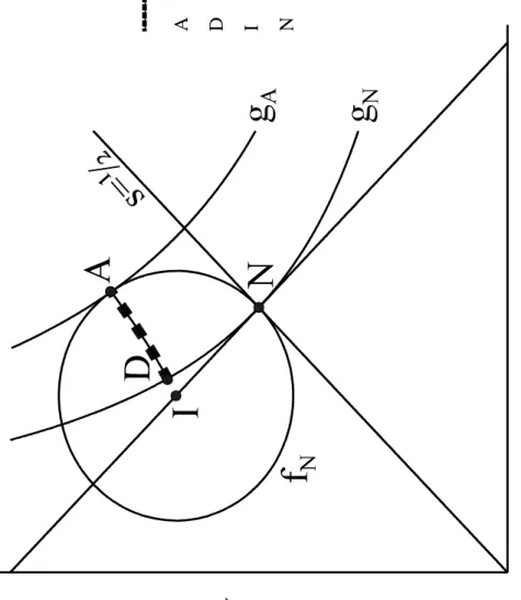
(8) for re-election.12 3. A Model of Agency-Donor Interaction This section presents a theoretical model to analyze the distribution of aid by a multilateral agency when (i) the agency relies on funding from an influential donor and (ii) the agency and donor have different preferences over benefit distribution. The model characterizes an agency that is dependent on a donor for funding, but can decide independently how to allocate funds between aid recipients. For simplicity, we consider the case of two recipients. Denote: x. Aid allocated to recipient x.. y. Aid allocated to recipient y.. B=x+y. Budget.. s=y/B. Budget share to recipient y.. "0[0,1]. Bargaining parameter measuring the donor bargaining position. "=0 indicates the agency has all the bargaining power and, thus, obtains all the gains from bargaining, i.e., the bargaining outcome is the point in the core favored by the agency (point A in Figure 1). "=1 indicates the donor has all the bargaining power, i.e., the bargaining outcome is the point in the core favored by the donor (point D in Figure 1).. Assumptions: A1. Donor Preferences. The donor maximizes the following objective function: f(x,y) = !(x!xI)2!(y!yI)2. where: 0<xI<yI. This generates circular indifference curves centered on the donor’s ideal point I=(xI,yI).13 A2. Agency Preferences. The agency’s objective function g(x,y) exhibits positive, diminishing returns and is symmetric and homothetic. This implies standard-shaped indifference curves, symmetric about x=y, smooth, convex, and with constant slope along a ray from the origin.14. 7.

(9) A3. Structure of Game. The donor selects the budget for the agency, which in turn allocates that budget between recipients x and y. If no bargaining occurs, policy is a simple Nash equilibrium in which the donor’s strategy is budget size (B) and the agency’s strategy is an allocation of shares (s). If bargaining occurs, the simple Nash equilibrium serves as the endowment point for determining the core; the donor and agency bargain to some point in the core. The bargaining outcome is denoted by s"="sD+(1!")sA where sD is the donor’s preferred share in the core and sA is the agency’s preferred share in the core.15. Policy Outcomes We present the model’s solution as propositions followed by a graphical illustration. These propositions explain how policy outcomes depend on whether or not bargaining occurs, on the relative bargaining power of the agency and the donor if bargaining does occur, and on donor preferences. Appendix A proves each proposition.. P1. Without bargaining, the donor does not influence allocation. Without bargaining, donor preferences influence only the total budget, not the share of the budget going to each recipient. The outcome will allocate the budget evenly between recipients: B=xI+yI, s=½.. P2. With bargaining, the donor does influence allocation. With bargaining, donor preferences influence the relative shares of aid going to recipients, not just the total aid budget: B>xI+yI, s>½.. P3. With bargaining, donor influence varies with bargaining power. With bargaining, bargaining power influences the share of aid going to each recipient. The share (s) for the donor’s favored recipient moves away from ½ as the bargaining power of the donor (") increases: Ms/M" > 0.. P4. With bargaining, the degree of donor bias influences allocation. All else equal, a higher donor ideal share to recipient y results in a higher value of s at the bargaining outcome. With sI=yI/(xI+yI): Ms/MsI > 0. [Figure 1 about here] In Figure 1, first consider the non-bargaining case. Faced with any fixed budget line, the. agency allocates aid evenly, as represented by the 45 degree line (s=½). This follows from the symmetry of the agency’s indifference curves. Given an agency strategy of an allocation along this 8.

(10) 45 degree line, the donor maximizes f by selecting the budget line running through its ideal point. Thus, in the absence of bargaining, the outcome is the simple Nash equilibrium (N in Figure 1), which allocates aid equally between the two recipients. The donor has no influence on aid allocation. If the agency and donor do bargain, the outcome will be in the core, where recipient x will receive less than will recipient y. An increase in the donor’s relative bargaining power (") will move policy along the core, so that policy moves away from A and toward D, yielding an increased value of f, a decreased value of g, and a higher value of s. Finally, if the donor’s ideal point shifts so that sI increases (decreases), the core shifts so that s increases (decreases).16 Applying the Model Practical application of the model requires controlling for aspects of recipient heterogeneity that the theoretical analysis omits. Most important are characteristics that enter official aid allocation criteria, such as differences in need and absorptive capacity. With Q representing these country characteristics and sWB representing a recipient’s share of World Bank lending, the model predicts: sWB=s(Q,",sI) where MsWB/M">0 and MsWB/MsI>0. Controlling adequately for country characteristics presents several challenges. To capture official aid allocation criteria, Q must include a large number of variables–only some of which will be available for the majority of developing countries.17 At the same time, broad sample coverage is important to minimize sample selection problems, particularly since we examine allocation between countries. The potential for selection bias is clear because countries with few published statistics tend to differ systematically from other countries and, thus, may correspond disproportionately to country x in the theoretical model.18 Our approach to this problem is to include both a limited set of widely available country 9.

(11) characteristics (Q) and the bilateral aid shares from a group of small donors (sSD). Numerous studies have found that these countries (Canada, Denmark, the Netherlands, Norway, and Sweden–sometimes termed “like-minded donors”) allocate their aid in a more humanitarian manner than do large donors such as the U.S., Japan, France, and the U.K. (Alesina and Dollar, 2000; Hoadley, 1980; McGillivray, 1989; Rao, 1997; Rodrik, 1995; Stokke, 1989).19 Furthermore, small donors have little direct influence over World Bank loan allocation. A contribution-based voting structure gives these countries little power on the Board of Executive Directors while, ironically, their willingness to contribute limits their influence during the triennial IDA replenishment. Thus, any link between small donor bilateral aid allocation and World Bank loan allocation is driven by common development concerns.20 We follow a similar approach to proxy for U.S. interests, using a set of U.S. interest variables Z and the U.S. bilateral aid share (sUS). These variables should reflect the U.S. ideal point (I) and hence identify the influence of sI on s (Proposition 3). While U.S. aid allocation notoriously reflects U.S. interests, it may not be entirely self-interested, hence the importance of including the humanitarian variables described above. The discussion above is summarized in the following aid allocation equation (suppressing country and time subscripts): sWB = Q$0 + sSD$1 + Z$2 + sUS$3 + ,. (1). With variables defined appropriately (e.g., higher Z indicating greater U.S. interest), the model predicts that $2=0 and $3=0 if there is no bargaining (i.e., no donor influence). With bargaining, the model predicts $2>0. In principle, U.S. influence could yield an ambiguous sign for $3. If U.S. policy is to use bilateral and multilateral aid as complements (i.e., the U.S. uses bilateral and. 10.

(12) multilateral aid to pursue the same objectives in the same countries), then U.S. influence means. $3>0. If the U.S. views them as substitutes (perhaps because the U.S. does not want to give visible support), then $3<0. It is possible that multilateral aid could be seen as a substitute in some cases and a complement in others.21 An important caveat to the discussion above is the question of the agency’s own biases.22 There is a substantial literature arguing that, even bracketing donor influence, the World Bank’s objective function is not exclusively developmental due to principal-agent problems and other bureaucratic factors (Martens et al., 2002). Numerous internal reports as well as work by academics (Kilby, 2000) find evidence of a “pressure to lend,” suggesting a bias toward new lending at the expense of development impact. In terms of our empirical work, these issues are relevant if World Bank institutional biases are correlated with but not caused by our measures of donor interest. However, constructing variables to proxy for such biases is challenging.23 Notably, much of the discussion of institutional biases (Tendler, 1975) focuses on the capital and import intensity of projects and on the overall level of lending rather than on biases toward or against particular recipient countries. Issues such as defensive lending are country-specific but difficult to disentangle from donor interest and recipient need. We might tell a purely bureaucratic story where a country would receive more funding if overall lending in its regional division within the World Bank were below target. But constructing a variable to capture this would require data not currently available. In short, institutional biases clearly exist and are important; how to capture them and the degree to which they might influence our results in this context remains an open question. 4. Data The dependent variable in the estimated equations is a country’s share of World Bank lending (sWB) and corresponds directly to its theoretical counterpart. It is defined as World Bank lending to 11.

(13) country i in year t, divided by World Bank lending to all included countries in year t. Lending is measured as “Total Official Gross,” i.e., gross disbursements of World Bank loans (IDA, IBRD, and IFC).24 Parallel to factors represented by Q in the previous section, all specifications include eleven variables to control directly for cross-recipient heterogeneity. Country size as measured by population is an important allocation criterion which may enter nonlinearly (e.g., a bias against large countries) so the estimated equation includes recipient country population as a share of population in included countries in a given year (POP), its square (POP2) and the population growth rate (POP_GROW). To control for poverty (and perhaps creditworthiness and the potential for aid effectiveness), three national income variables are included: per capita GDP (GDP), its square (GDP2), and growth rate (GDP_GROW). Three trade-related variables–an index of openness (OPEN), share of world exports (WORLD_EX), and share of world imports (WORLD_IM)–reflect the quality of the policy environment and the country’s importance in world trade.25 Finally, two variables capture commercial financial flows: (i) the net flow (where positive) into the country as a share of net commercial flows (where positive) into all included countries that year (WORLD_COMP) and (ii) the net flow (where positive) out of the country as a share of net commercial flows (where positive) out of all included countries that year (WORLD_COMN). These variables may reflect access to world capital markets as well as financial crises. Inclusion of the world trade and financial variables is particularly important as we use parallel U.S.-only variables to reflect U.S. interests. Proxies for the U.S. ideal point include four U.S. commercial interest variables (corresponding to Z). Two variables reflect trade with the U.S.: U.S. exports to the country as a share of U.S. exports to all included countries (US_EX) and U.S. imports from the country as a share 12.

(14) of U.S. imports from all included countries (US_IM). These variables reflect the country’s importance to the U.S. as a trade partner while allowing for imports and exports to play different roles (as suggested by the politics of trade policy). The other two variables are based on U.S. commercial financial flows: (i) the net flow (where positive) into the country as a share of net U.S. flows (where positive) into all included countries that year (US_COMP) and (ii) the net flow (where positive) out of the country as a share of net U.S. flows (where positive) out of all included countries that year (US_COMN).26 Ex ante, large flows in either direction might give the U.S. an incentive to encourage lending to a country. As explained in Section III, we use two bilateral aid variables to capture additional humanitarian and donor interest factors. sUS is U.S. bilateral aid to country i in year t as a share of U.S. bilateral aid to all included countries in year t. sSD is small donor bilateral aid to country i in year t as a share of small donor bilateral aid to all included countries in year t. [Table 1 about here] Table 1 presents descriptive statistics. The panel of 3035 annual observations covers 110 countries between 1968 and 2002.27 The dependent variable sWB, the share of World Bank lending a country receives, averages just over 1%; 345 observations have sWB=0 while the maximum of 25.1% is India in 1968. In view of the range in observed values for both the dependent and independent variables in Table 1, an important econometric concern is the presence of influential outliers.28 For this reason, we test the robustness of all results to the treatment of outliers. In some cases, results do change and are so noted. 5. Empirical Results We estimate the World Bank share equation (1) via feasible generalized least squares with an AR1 error structure. Because the number of countries is greater than the number of years, we must restrict 13.

(15) the autocorrelation parameter to be the same across panels (Beck and Katz, 1995). Table 2 presents estimates based on the full sample. Column 1 is the most basic specification omitting the bilateral aid proxies for U.S. interests (sUS) and development concerns (sSD) as well as commercial financial flows. Column 2 adds sUS and sSD while Column 3 adds commercial financial flows.29 [Table 2 about here] The column 1 coefficients on official aid allocation variables (POP, POP2, POP_GROW, GDP, GDP2, GDP_GROW, OPEN, WORLD_EX, WORLD_IM) are typical of estimates for these variables in other specifications and samples. The estimated coefficient for POP is positive and significant both statistically and in terms of magnitude, indicating that country size is a major determinant World Bank funding levels. The negative, significant quadratic term is indicative of a bias against large countries (notably India and China).30 Population growth is insignificant (conditional on the other included variables). The positive linear and negative quadratic terms for per capita GDP suggest a slight middle income bias (with aid share peaking around a GDP per capita of $4,500 in purchasing power parity terms). However, if we restrict variables to ±2 standard deviations from their means, neither term is significant (individually or jointly in specifications for Columns 1, 2, or 3). In practice, the data restriction affects only the high GDP per capita observations. Thus, if we limit the influence of high income countries which receive very little World Bank funding, income is not an important determinant of World Bank flows within the group of borrowing countries.31 Neither GDP growth nor openness are significant (again, conditional on the other included variables). World trade shares (WORLD_EX and WORLD_IM) enter positively but neither is significant. However, both variables are significant if we limit the influence of larger traders. WORLD_EX enters with a coefficient of 14.

(16) 0.337, significant at the 1% level, while WORLD_IM enters with a coefficient of -0.185, significant at the 5% level. Other coefficient estimates (notable, U.S. trade variables) do not depend on the restriction of world trade. U.S. exports enter significantly in all three specifications, consistent with Frey and Schneider (1986). The effect is substantial; a one standard deviation increase in U.S. export share (from 1.0% to 3.9%) is associated with a increase in World Bank aid share from 1.1% to 1.7%, ceteris paribus. As with the world export variable, the estimated coefficient on U.S. exports is somewhat larger when we restrict the influence of outliers. Note that WORLD_EX includes U.S. exports so that the estimated coefficient on US_EX is the differential effect of U.S. trade relative to trade in general.32 US_IM enters with a negative sign but is not significant. The signs of these variables are consistent with the role that exports and imports play in U.S. trade politics. Turning to Column 2, small donor bilateral aid share (sSD) enters positively and significantly. Since small donors lack the power to influence World Bank lending decisions, this is best interpreted as reflecting developmental concerns not captured by the other variables. U.S. bilateral aid share also enters positively and significantly. A one standard deviation increase in sUS (from 1.1% to 3.3%) is associated with an increase in World Bank aid share from 1.1% to 1.2%, a relative small increase.33 Given the strength of the link between U.S. trade interests and World Bank lending, this weaker result may reflect aid instruments that are sometimes complements and sometimes substitutes. Column 3 adds our measures of commercial financial flows. WORLD_COMP enters with a negative and significant coefficient indicating that inflows of commercial funds are associated with less new lending from the World Bank. The positive coefficient on WORLD_COMN is consistent with this though not statistically significant. The U.S. financial variables enter with the opposite 15.

(17) signs: net flows from the U.S. to the country are associated significantly with more World Bank lending while net flows to the U.S. have a negative though insignificant link with World Bank flows. This link is driven mainly by large flows and becomes statistically insignificant (though with the same sign) if we restrict the influence of outliers.34. As with trade, WORLD_COMP and. WORLD_COMN include commercial financial flows into and out of the U.S. so the coefficients on US_COMP and US_COMN indicate the differential effect for the U.S. variables.35 We explore the magnitude of the impact of U.S. interest variables and recipient need variables in simulations. If we increase statistically significant U.S. interest variables (US_EX, sUS and US_COMP) by one standard deviation, the World Bank lending share for an otherwise average country is predicted to increase by about a half from 1.13% to 1.76%, nearly double the effect for non-U.S. variables exclusive of population (WORLD_COMP and sSD). Country size is also very important: a one standard deviation increase in population share corresponds to a 2.8 fold increase in lending share.36 To assess how U.S. influence has changed over time, we estimate separate equations by presidential administrations (Johnson through George W. Bush). This approach allows for differences in the perceptions of U.S. interests and changing strategies to meet these ends (i.e., movements in the U.S. ideal point I). It also allows for gradual changes in the bargaining position of the U.S. relative to the World Bank. A breakdown by administration is particularly relevant given the previous literature on donor influence. Table 3 presents results, while Table 4 summarizes this information for U.S. interest variables and indicates robustness to treatment of outliers. [Table 3 about here] Missing data until 1968 limit the Johnson administration sample to 74 observations.37 Of the non-U.S. variables, WORLD_COMN and sSD enter significantly. During this period (1968), 16.

(18) outflows of commercial funds were linked with less World Bank lending, a result which is robust to the treatment of outliers. An increase in WORLD_COMN by one standard deviation from the mean of 1% to 5% results in a predicted decrease in World Bank lending share from 1.3% to 0.3%.38 There is a strong positive and robust link between small donor aid and World Bank lending; an increase in small donor share by one standard deviation from the mean of 1.3% to 5.5% results in a sizeable predicted increase in World Bank lending share from 1.3% to 3.7%. Turning to U.S. interest variables, there is a positive and significant link between U.S. exports and World Bank lending; an increase in U.S. export share by one standard deviation from the mean of 1.2% to 3.5% results in a predicted increase in World Bank lending share from 1.3% to 2.5%. However, this is entirely driven by larger traders. Negative U.S. commercial flows are also linked to higher World Bank lending; an increase in US_COMN by one standard deviation from the mean of 1% to 5.7% results in a predicted increase in World Bank lending share from 1.3% to 2.2%. This link is robust to treatment of outliers. Taken together, the significant recipient need variables appear to play a somewhat larger role than the U.S. interest variables during this last year of the Johnson administration. Interestingly, the magnitude of the coefficients on sUS and sSD is substantially higher than when using the full time series.39 The first Nixon administration from 1969 to 1972 provides a richer data set with 304 observations. From the Nixon administration on, population plays the same role as in the overall sample with significant positive linear and negative quadratic terms. WORLD_COMP enters positively and significantly though this result is driven by outliers; an increase in WORLD_COMP by one standard deviation from the mean of 1.2% to 4.4% results in a predicted increase in World Bank lending share from 1.3% to 1.8%. Small donor share is positive and significant while none of the U.S. interest variables are significant; an increase in small donor share by one standard deviation 17.

(19) from the mean of 1.3% to 4.9% results in a predicted increase in World Bank lending share from 1.3% to 2.1%. The Nixon/Ford administration from 1973 to 1976 has similar sample coverage with 323 observations. Two U.S. interest variables are significant in this period. U.S. export share is positive and significant, mostly due to the influence of large trading partners. An increase in U.S. export share by one standard deviation from the mean of 1.1% to 3.3% results in a predicted increase in World Bank lending share from 1.2% to 1.8%. U.S. aid share is also positive and significant, a result that does not depend on the influence of outliers. However, the size of this effect is small; an increase in U.S. aid share by one standard deviation from the mean of 1.1% to 2.2% results in a trivial predicted increase in World Bank lending share from 1.2% to 1.3%. Interestingly, small donor aid share is not significant in the period even if U.S. aid share is omitted. The Carter administration from 1977 to 1980 includes 329 observations. In both the Carter and first Reagan administrations, GDP per capita enters significantly with World Bank loan share increasing with income up to about $4,800. As mentioned in the discussion of Table 2, this analysis does not consider differences between IDA and IBRD concessionality so that we cannot draw conclusions about the World Bank’s poverty orientation from this. The effect also proves very small; an increase in GDP per capita by one standard deviation from the mean of $3,200 to $5,700 results in a minuscule predicted increase in World Bank lending share from 1.2% to 1.21%. World import share enters negatively and significantly during this period; an increase in World import share by one standard deviation from the mean of 0.8% to 2% results in a predicted decrease in World Bank lending share from 1.2% to 0.7%. sSD returns as a significant factor though with a modest impact; an increase by one standard deviation from its mean of 1.1% to 3.2% results in a predicted increase in World Bank lending share from 1.2% to 1.4%. Turning to U.S. interest variables, the estimated 18.

(20) coefficient for US_EX is again positive and significant but is heavily influenced by larger trading partners. An increase in U.S. export share by one standard deviation from the mean of 1% to 3.2% results in a predicted increase in World Bank lending share from 1.2% to 1.8%. The negative and significant coefficient on US_COMN is likewise driven by extreme values; an increase of one standard deviation from the mean of 1.1% to 6.2% results in a predicted decrease in World Bank lending share from 1.2% to 0.2%. As in the previous Ford administration, sUS enters positively, significantly and robustly suggesting a policy of using bilateral and multilateral aid as complements rather than substitutes. The magnitude of this effect is somewhat larger; an increase in U.S. aid share by one standard deviation from the mean of 1.2% to 3.2% results in a predicted increase in World Bank lending share from 1.2% to 1.5%. For the first Reagan Administration from 1981 to 1984 (332 observations), population, GDP and world import share continue to play a similar role as in the previous four years. U.S. trade appears to play a more important role with US_EX positive, significant and robust while US_IM is negative, significant though not robust. A one standard deviation increase in the former (from the mean of 1% to 3.3%) results in a predicted increase in World Bank lending share from 1.2% to 1.9% while a one standard deviation increase in the latter (from the mean of 1.1% to 3.5%) results in a decrease in World Bank lending share from 1.2% to 0.7%. Both sUS and sSD are small and insignificant in this period though this depends to some extent on influential outliers. In the case of the U.S., a large portion of the aid budget went to Mexico in 1982, a pattern not mirrored by World Bank disbursements. During the second Reagan Administration from 1985 to 1988 (335 observations), World Bank lending patterns continue to reflect U.S. trade interests. As in the previous administration, the coefficient on US_EX is large, positive, significant and robust while the coefficient on US_IM is 19.

(21) large, negative and significant but is driven primarily by larger trading partners. A one standard deviation increase in the former (from the mean of 1.1% to 3.9%) results in a predicted increase in World Bank lending share from 1.2% to 2.8% while a one standard deviation increase in the latter (from the mean of 1.1% to 3.9%) results in a marked decrease in World Bank lending share from 1.2% to 0.1%. The relationship of U.S. aid and World Bank lending as substitutes previously evident in the case of Mexico in 1982 is clear in this period: the coefficient on sUS is negative, significant and robust. A second large infusion of U.S. aid to Mexico in 1987 plays a role in this but even omitting Mexico altogether the estimated coefficient remains negative and significant. The magnitude of this link is, however, modest; an increase in U.S. aid share by one standard deviation from the mean of 1.1% to 2.9% results in a predicted decrease in World Bank lending share from 1.2% to 1.0%. As in the previous period, the estimated coefficient on small donor aid share is small and insignificant due to some influential outliers (principally, Tanzania and Bangladesh). During the elder Bush Administration from 1989 to 1992 (343 observations), commercial financial flows appear to play a substantial role. WORLD_COMP enters negatively and significantly but is not robust to the treatment of outliers (again, with Mexico playing a key role). An increase in WORLD_COMP by one standard deviation from the mean of 1.1% to 3.9% results in a predicted decrease in World Bank lending share from 1.1% to 0.7%. WORLD_COMN enters positively and significantly and is robust to the treatment of outliers; a one standard deviation increase (from the mean of 1% to 5%) results in a predicted increase in World Bank lending share from 1.1% to 1.7%. U.S. commercial flows enter with the opposite signs, US_COMP robustly. An increase in US_COMP by one standard deviation from the mean of 1.1% to 5.6% results in a predicted increase in World Bank lending share from 1.1% to 1.4%. Thus, during this period the World Bank tended to lend more when investors fled and less when private money was plentiful though these effects 20.

(22) were substantially reduced when U.S. finances were involved. U.S. exports once again enter as positive, significant, and robust but, unlike the previous period, imports appear to play no role. The export effect is substantial with a one standard deviation increase from the mean (1.1% to 4.3%) predicting an increase in World Bank lending share from 1.1% to 2.2%. Small donor aid share, always entering positively, is once again significant and robust though small; an increase in small donor aid share by one standard deviation from the mean of 1.1% to 2.8% results in a predicted increase in World Bank lending share from 1.1% to 1.3%. Perhaps in transition from the policy under Reagan, U.S. aid share plays no role, entering with a small and insignificant coefficient regardless of the treatment of outliers. The first Clinton administration from 1993 to 1996 has 406 observations on 104 countries. It is the only period in which the index of openness is significant with more open economies receiving less World Bank funding. This result is not robust, however, with most of the effect driven by Singapore and the effect is quite small; an increase in openness by one standard deviation from the mean of 75% to 121% results in a predicted decrease in World Bank lending share from 1% to 0.9%. WORLD_EX is negative and significant but not robust to treatment of outliers; in fact, if we exclude the larger traders (China, Korea, Mexico, Singapore, Malaysia, and Thailand), WORLD_EX becomes positive and significant. As during the previous period, sSD is positive, significant and robust but again the magnitude of the effect is small. WORLD_COMP is positive and significant but again not robust to the treatment of outliers; an increase by one standard deviation from the mean of 1% to 2.4% results in a predicted increase in World Bank lending share from 1% to 1.2%. Turning to U.S. interests, U.S. exports do not play a significant role while U.S. imports enter as positive and significant (though the impact is small) when including large suppliers (China, Korea, Mexico, Singapore) but negative and significant excluding them. sUS is positive and significant but 21.

(23) the effect is small and not robust to treatment of outliers. Net inflows of private U.S. funds (US_COMP) have a positive, significant and robust link to World Bank lending in this period; an increase of one standard deviation from the mean of 1% to 4.2% results in a predicted increase in World Bank lending share from 1% to 1.5%. The dramatic changes taking place during this period, with aid to transition economies becoming significant and Cold War patterns being rethought, is underscored by the large negative estimated autocorrelation coefficient (D=!.8657). The strongest trade links are apparent in the second Clinton administration from 1997 to 2000 (396 observations on 102 countries). Countries that purchased a larger share of world exports received significantly less World Bank funds (though this depends heavily on Korea) while those that provided the world with more imports got significantly more. Both effects are relatively large. A decrease in world export share from one standard deviation above the mean (2.6%) to the mean (0.8%) results in a sizeable predicted increase in World Bank lending share from the mean of 1% to 2.9%.40 An increase in world import share by one standard deviation from the mean of 0.9% to 3.1% results in a predicted increase in World Bank lending share from 1% to 4.7%. The differential effect for U.S. exports is significant and positive (but depends heavily on Mexico) while the effect for U.S. imports is significant and negative. Again, both effects are large. An increase in U.S. export share by one standard deviation from the mean of 0.9% to 4.4% results in a sizeable predicted increase in World Bank lending share from the mean of 1% to 3.7%. A decrease in U.S. import share from one standard deviation above the mean (4.1%) to the mean (0.9%) results in a predicted increase in World Bank lending share from 1% to 4.4%. The only other significant covariate in this period (other than population) is WORLD_COMP which enters as positive, significant and robust to the treatment of outliers; an increase of one standard deviation from the mean of 0.9% to 3.4% results in a predicted increase in World Bank lending share from 1% to 1.6%. 22.

(24) The final column of Table 3 covers the beginning of the junior Bush’s first administration from 2001 to 2002 (182 observations on 91 countries). Both world trade variables are significant (WORLD_EX positive, WORLD_IM negative) but sensitive to the treatment of large traders including Russia. An increase in the world export share by one standard deviation from the mean of 0.9% to 2.9% results in a predicted increase in World Bank lending share from 1% to 3.7%. A decrease in world import share from one standard deviation above the mean (3.4%) to the mean (0.9%) results in a predicted increase in World Bank lending share from 1% to 3.5%. WORLD_COMN enters the estimated equation with a positive, significant coefficient but again this is not robust to the treatment of outliers. The effect is also more modest in size; an increase in WORLD_COMN by one standard deviation from the mean of 0.9% to 4.4% results in a predicted increase in World Bank lending share from 1% to 1.3%. Finally, US_COMN also enters with a positive, significant but not robust coefficient; the magnitude of this effect is roughly the same as for WORLD_COMN. [Table 4 about here] Table 4 summarizes statistical significance and robustness for the U.S. interest variables across the administrations. U.S. export share is significant and positive in seven of the ten administrations, robustly so in two and having a substantial effect in many cases. U.S. import share is significant in four cases, negatively in three and positively in one (due to a few large trading partners). U.S. aid share also enters significantly in four administrations (positively in three, negatively in one) and generally has a smaller apparent impact than trade. This evidence is consistent with bilateral and multilateral aid acting as substitutes in some cases and as complements in others. The link between U.S. commercial financial flows and World Bank lending proves highly variable; these flows generally appears to play a smaller role than trade flows.41 23.

(25) 6. Conclusion The empirical analysis, motivated by a model of agency-donor interaction, yields results largely consistent with significant U.S. influence over World Bank lending, but through evolving rather than stable relationships. U.S. interests in and policy toward the World Bank change frequently with presidential administrations and with economic and political circumstances. Taking the 1968 to 2002 period as a whole, two measures of U.S. interests have a significant and robust link with World Bank lending allocations. The first relates to trade. While there is no apparent link with world trade, the differential impact of purchasing of U.S. exports is positive: ceteris paribus, the greater the share of U.S. exports that a country purchased, the more funds the country got from the World Bank. This is consistent with the political economy of trade in the U.S. which favors exports over imports. The second significant measure may be interpreted as geopolitical. After including a number of controls for development concerns, we find countries favored in U.S. bilateral aid allocations also received a disproportionate share of World Bank funds. These aggregate results mask significant variation across the period, both in U.S. policy toward the World Bank and in underlying U.S. interests. From the Johnson administration through the first Bush administration, the link with U.S. exports remains positive and, except in Nixon’s first term, significant. The first Clinton administration saw a change with a negative though insignificant relationship, reflecting large aid flows to transition economies which had no established trade ties with the U.S. The years since then suggest this may be a transitory pattern with trade interests reemerging as a significant influence. The relative consistency of the trade variable, as compared to the financial flow indicators, mirrors the more long term nature of trade ties. The link between U.S. aid and World Bank lending is more variable; we would expect this since bilateral and multilateral aid are distinct foreign policy tools. In many situations when a 24.

(26) powerful donor wishes to fund a recipient country, it would provide its own funds and pressure the multilateral agency to supplement these. However, in some cases, the logic is reversed, for example when the donor cannot publically support the recipient. This may explain why U.S. bilateral aid enters positively and significantly in the Ford, Carter, and first Clinton administrations but negatively and significantly in the second Reagan administration. Taken as a whole, the empirical evidence points to U.S. influence over the World Bank, influence used in direct pursuit of U.S. economic and strategic interests. These links are substantial though not overwhelming.42 Nonetheless, when a multilateral organization serves the narrow interests of a powerful member, its unique character–its legitimacy–is necessarily eroded. Equally, the ability to credibly commit to future policies is reduced as donor objectives change with its domestic political cycle. This poses a critical problem for the World Bank and its current pursuit of selectivity. The policy of ex post conditionality promises substantial funding for developing countries governments only after reforms have taken place. Governments’ willingness to do this depends heavily on faith in the reform package and the implicit promise of future loans, that is, on the World Bank’s legitimacy and credibility.. 25.

(27) Appendix A: Proofs of Propositions 1-4 The proofs below use the same notation as in Figure 1. Proposition 1: The no-bargaining Nash Equilibrium is B=xI+yI and s=½. Proof: For any fixed budget B (a budget line with slope=!1), the agency’s symmetric preferences imply equal shares for countries x and y, i.e., s=½. Taking s=½ as given (because it is a dominant strategy for the agency), the donor maximizes its objective function f subject to the constraints B=x+y and x=y. Applying elementary calculus or geometry yields B=(xI+yI).9 Proposition 2: With bargaining, B>xI+yI and s>½. Proof: If C is a point in the core and thus in the lens, it must satisfy f(C)$f(N). The point N occurs at a tangency between the donor indifference curve fN and the s=½ line. These two characteristics preclude from the lens, and hence from the core, (i) all points below the s=½ line and (ii) all points on the s=½ line except N. N can be easily ruled out of the core as mutual gains from bargaining remain unexploited at N where (Mf/Mx)/(Mf/My)=!1, while (Mg/Mx)/(Mg/My)=1. Hence, for all points in the core, s>½. A similar argument demonstrates that xC+yC>xI+yI, i.e., for all points in the core, B>xI+yI.9 Before proving Proposition 3, it is useful to prove a preliminary lemma. First, define sI=yI/(xI+yI), the share for country y at the donor’s ideal point. In general, sK denotes the value of s at point K (i.e., sK=yK/(xK+yK)) as well as the ray from the origin through point K (which has slope=sK). Lemma 1: The entire core lies above the line s=½ and below the line s=sI. Proof: Proposition 2 shows that the entire core has s>½, which implies (Mg/Mx)/(Mg/My)>1. Since (Mf/Mx)/(Mf/My)>1 only below the line parallel to s=½ through I, the core must lie in the portion of the lens below this line and above the line s=½. This region is a subset of the lens, above the line s=½ and below the line s=sI, which proves the lemma.43 9 Proposition 3: With bargaining, Ms/M">0. Proof: Agency indifference curves have constant slope along rays from the origin with the absolute value of the slope of the indifference curve directly related to the slope of the ray. Donor indifference curves have constant slope along rays from the ideal point (I) with the absolute value of the slope of the indifference curve inversely related to the slope of the ray (in the relevant range). Lemma 1 shows that all rays from the origin to points in the core will fall below sI. Thus, for any point C0 in the core, the ray sC0 from the origin will be steeper than the ray rC0 from the donor’s ideal point.44 See Appendix Figure A1. Consider a second point in the core C1, such that g(C1)<g(C0). The rays from the origin and the donor’s ideal point are not co-linear so at least one ray must differ from the previous case to have an intersection at C1. Since the slopes of the agency and donor indifference curves must be equal 26.

(28) at C1 yet change in opposite directions relative to the slopes of the two rays, we must have sC1 steeper than sC0 and rC1 less steep than rC0. This proves that s, slope of the ray from the origin and the share to country y, increases monotonically as we move along the core from the agency’s preferred point to the donor’s preferred point. In terms of the bargaining parameter, s increases montonically as " increases from the agency’s preferred point in the core (A where "=0) to the donor’s preferred point in the core (D where "=1): Ms/M">0.45 9 [Appendix Figure A1 about here] Proposition 4: The degree of donor bias influences allocation: Ms/MsI>0. Proof: Given the bargaining structure, it is sufficient to show that an increase in sI will increase s at both endpoints of the core (D and A). Any change in I can be decomposed into a movement along the original budget line to the new value of s and then a movement along a ray from the origin out to the final point preserving that value of s. The second step (increasing the sum xI+yI without changing s) has no effect on the values of s in the core, allowing us to consider only the effect of the first step.46 First consider D. This point is defined by the tangency of a donor indifference curve and the agency indifference curve gN. Because the donor’s budget line does not change, the no-bargaining Nash equilibrium and hence gN do not change. To demonstrate that sA increases as sI increases, first construct a ray from the original donor ideal point I to the original tangency point D. Next, construct a ray from the new donor ideal point I' to D. The original and new donor indifference curves have constant but different slopes along these rays and, hence, the new donor indifference curve through D cannot be tangent to gN. Because the slope of the new donor indifference curve is greater than that of gN at this point, the point of tangency must be at higher y/x (equivalently, higher s) since moving in this direction increases the slope of gN while decreasing the slope of the indifference curve for f.47 The proof for the agency’s preferred point in the core (A) is best visualized geometrically (see Appendix Figure A2). Define sA to be both the ray from the origin through A and the slope of that ray. Denote by fN the initial donor indifference curve passing through the simple Nash equilibrium point and fN' the new donor indifference curve. By virtue of being in the core, A is the tangency between fN and an agency indifference curve (labeled gA). Traveling out along sA to point H, indifference curves for the agency maintain the same slope because of homothetic agency preferences. However, the same is not true for the new donor indifference curve fN' which is steeper at H. Since fN' become flatter and agency indifference curves become steeper as we move up fN', the tangency will occur above sA and, thus, sA'>sA.9 [Appendix Figure A2 about here]. 27.

(29) Appendix B: Data. Variable Definitions and Data Sources Coverage: All aid-receiving countries are included subject to data availability (including OECD’s DAC database) except for Egypt after 1978 and Israel. Countries are defined as those appearing in the Polity IV database (i.e., the Polity2 variable must be available). This excludes territories and colonial possessions which do have separate trade and macro data in some cases. Calculation of shares: Country i is included in share calculations for year t if all country i’s share variables are available in year t. Thus, a country missing POP_GROW, GDP or OPEN data in a given year may still be included in the denominator of the share calculations even though it drops from the regression that year. A country would not be included that year if any of its share variables (sWB, POP, WORLD_EX, WORLD_IM, sSD, WORLD_COMP, WORLD_COMN, US_EX, US_IM, sUS, US_COMP, US_COMN) are missing that year. Thus, all share variables have consistent denominators. Inclusion of year dummies deals with cases where yearly shares do not sum to 1. Dependent Variable sWB: World Bank lending to country i in year t / total World Bank lending to all included countries in year t; lending measured as “Total Official Gross.” Data for 1968 are missing for multilateral institutions, presumably because of a change-over from calendar to fiscal years. We use the average of 1967 and 1969. Correction of data “errors”: “Total Official Gross” = max(Total Official Gross, Total Official Net, 0). Only a few data points were affected. (OECD DAC database) Control Variables POP: Population of country i in year t / total population in all included countries in year t. (Penn World Tables and WDI) POP_GROW: Annual growth rate of population in country i between year t-1 and t. (Penn World Tables and WDI) GDP: Purchasing power parity GDP per capita in country i in year t. Constant thousands of dollars (Chain Index, expressed in international prices, base year 1996). (Penn World Tables and WDI) GDP_GROW: Annual growth rate of above GDP variable in country i between years t-1 and t. (Penn World Tables and WDI) OPEN: Trade relative to GDP: (imports+exports)/GDP. (Penn World Tables and WDI) WORLD_EX: Exports from other countries to country i in year t / total of exports from other countries to each included country in year t. (IMF DOTS). 28.

(30) WORLD_IM: Imports into other countries from country i in year t / total of imports into other countries from each included country in year t. (IMF DOTS) sSD: Small donor bilateral aid to country i in year t / total small donor bilateral aid to all included countries in year t; aid measured as “Total Official Gross.” Same error correction as for the dependent variables. Small donors are: Canada, Denmark, Netherlands, Norway, Sweden. (OECD DAC database) WORLD_COMP: Net commercial financial flows into country i in year t / net commercial financial flows into all included countries in year t. Mathematically, let Di,t=max[(Total Resources Neti,t!Total Official Neti,t),0]. Then WORLD_COMP=Di,t/. Dj,t. (OECD DAC database). WORLD_COMN: Net commercial financial flows out of country i in year t / net commercial financial flows out of all included countries in year t. Mathematically, let Di,t=min[(Total Resources Neti,t ! Total Official Neti,t),0]. Then WORLD_COMN=Di,t/. Dj,t. (OECD DAC database). U.S. Interest Variables US_EX: U.S. exports to country i in year t / total U.S. exports to all included countries in year t. (IMF DOTS) US_IM: U.S. imports from country i in year t / total U.S. imports from all included countries in year t. (IMF DOTS) sUS: U.S. bilateral aid to country i in year t / total U.S. bilateral aid to all included countries in year t; aid measured as “Total Official Gross.” Same error correction as for the dependent variable. (OECD DAC database) US_COMP: Net U.S. commercial financial flows into country i in year t / net U.S. commercial financial flows into all included countries in year t. Mathematically, let Di,t=max[(Total Resources Neti,t!Total Official Neti,t),0]. Then US_COMP=Di,t/. Dj,t. (OECD DAC database). US_COMN: Net U.S. commercial financial flows out of country i in year t / net U.S. commercial financial flows out of all included countries in year t. Mathematically, let Di,t=min[(Total Resources Neti,t ! Total Official Neti,t),0]. Then US_COMN=Di,t/. 29. Dj,t. (OECD DAC database).

(31) Extreme Values The first group of explanatory variables in Table 1 reflects official aid allocation criteria. As with the dependent variable, all share variables average around 1%; the means differ slightly from each other because the number of countries varies over time. Population share (POP) ranges from a low of nearly zero for Equatorial Guinea in 1978 to a high of nearly 32% for China in 1971. Population growth (POP_GROW) averages 2.1% per year with the reported population figure for Rwanda shrinking by nearly 31% in 1994 and rising by 24% in 1997. Real GDP per capita in 1996 dollars (GDP) averages just under $3600 and ranges from $281 in Zaire in 1997 to $24,939 in Singapore in 1996. Real GDP per capita growth (GDP_GROW) averages 1.4%, running from a reported low of -42% for Rwanda in 1994 to a reported high of 78% for Equatorial Guinea in 1997. Our index of openness (OPEN) averages .65 with a low of .04 for China in 1970 and a high of 4.39 for Singapore in 1980. World export share (WORLD_EX) ranges from a low of 0 for Botswana in 1968 to a high of 15.6% for China in 2002. World import share (WORLD_IM) ranges from a low of 0 for Botswana in 1968 to a high of 21.5% for China in 2002. Small donor aid share (sSD) peaks at 32% for India in 1968. The share of net positive world commercial flows (WORLD_COMP) reaches 38% for Mexico in 1984 while the share of net negative world commercial flows (WORLD_COMN) reaches 62% for Chile in 1971. U.S. interest variables appear in the lower portion of Table 1. U.S. export share (US_EX) ranges from a low of 0 (83 observations) to a high of 38% for Mexico in 2000. U.S. import share (US_IM) ranges from a low of 0 (164 observations) to a high of 26% for Mexico in 2001. U.S. aid share (sUS) peaks at 35% for Poland in 1991. The share of net positive U.S. commercial flows (US_COMP) reaches 53% for Mexico in 1984 while the share of net negative U.S. commercial flows (US_COMN) reaches 91% for Venezuela in 1983.. 30.

(32) Appendix B (continued): Sample Coverage Country Albania Algeria Angola Argentina Armenia Azerbaijan Bangladesh Belarus Benin Bolivia Botswana Brazil Bulgaria Burkina Faso Burundi Cambodia Cameroon C.A.R. Chad Chile China Colombia Comoros Congo Costa Rica Croatia Cuba Cyprus Czech Republic Dominican Rep. Ecuador Egypt El Salvador Equatorial Guinea Estonia Ethiopia Fiji Gabon Gambia Georgia Ghana Guatemala Guinea Guinea-Bissau Guyana Haiti Honduras Hungary India Indonesia Iran Ivory Coast Jamaica Jordan Kazakhstan. Span 1992-02 1968-02 1975-96 1968-02 1993-02 1995-02 1972-02 1993-02 1968-02 1968-02 1968-99 1968-02 1992-02 1968-02 1968-02 1994-99 1968-02 1968-98 1968-02 1968-02 1968-02 1968-02 1975-02 1968-02 1968-02 1996-02 1986-96 1968-96 1993-02 1968-02 1968-02 1968-78 1968-02 1968-00 1993-02 1968-02 1970-99 1968-02 1968-02 1997-02 1968-02 1968-02 1968-02 1974-02 1968-99 1968-98 1968-02 1971-02 1968-02 1968-02 1968-02 1968-02 1968-02 1968-02 1995-02. Years 11 35 22 35 10 8 31 10 35 35 32 35 11 35 35 6 35 31 35 35 35 35 28 35 35 7 11 29 10 35 35 11 35 33 10 35 30 35 35 6 35 35 35 29 32 31 35 32 35 35 35 35 35 35 8. Country Kenya Korea, Rep. Kyrgyz Republic Latvia Lesotho Lithuania Macedonia Madagascar Malawi Malaysia Mali Mauritania Mauritius Mexico Moldova Morocco Mozambique Namibia Nepal Nicaragua Niger Nigeria Pakistan Papua New Guinea Paraguay Peru Philippines Poland Romania Russia Rwanda Senegal Sierra Leone Singapore Slovakia Slovenia South Africa Sri Lanka Swaziland Syria Tajikistan Tanzania Thailand Togo Trinidad & Tobago Tunisia Turkey Uganda Ukraine Uruguay Uzbekistan Venezuela Zaire Zambia Zimbabwe. 31. Span 1968-02 1968-02 1995-02 1992-02 1989-02 1994-02 1993-02 1968-02 1968-02 1968-02 1968-02 1968-99 1968-02 1968-02 1996-02 1968-02 1975-02 1990-99 1968-02 1968-02 1968-02 1968-02 1968-02 1975-99 1968-02 1968-02 1968-02 1980-02 1968-02 1992-02 1968-02 1968-02 1968-96 1968-96 1993-02 1993-02 1968-02 1968-02 1997-02 1968-02 1997-02 1968-02 1968-02 1968-02 1968-02 1968-02 1968-02 1968-02 1992-02 1968-02 1995-96 1968-02 1968-97 1968-02 1970-01. Years 35 35 8 11 14 9 10 35 35 35 35 32 35 35 7 35 28 10 35 35 35 35 35 25 35 34 35 23 35 11 35 35 29 29 10 10 35 35 6 35 6 35 35 35 35 35 35 34 11 35 2 35 30 35 32.

(33) Endnotes 1. Klitgaard et al. (2005) call the impact of aid targeting on the overall aid budget the “fundraising effect.” 2. Rodrik (1995) notes that independence lends credibility to multilateral agencies’ policy advice (conditionality) while also strengthening their information signaling role. He argues that signaling and conditionality are the only economic rationale for multilateral development banks (MDBs) given international capital markets and bilateral aid agencies; an obvious corollary is that this rationale depends on MDBs’ independence. Taking a principal-agent approach to the delegation problem (why states delegate power to international organizations [IOs]), Thompson (2003, 2) states that “variation in institutional independence constitutes the most important characteristic defining the ‘nature of the agent,’ and it largely determines the mixture of costs (agency slack and loss of control) and benefits (increased support and legitimacy) achieved by the principal.” Hawkins et al. (2003) include credibility of policy commitments as a central benefit of delegating power to IOs, drawing parallels to the literature on central bank independence as the solution to a time-inconsistency problem. Thompson and Haftel (2003) argue that the costs to states of independent IOs are balanced by the benefits of independence including increased bargaining power and credibility. In addition, the neutrality of independent IOs allows for more reliable information, unbiased expertise, and “allows them to confer legitimacy upon actions that receive their endorsement” (Thompson and Haftel, 2003, 2-3). 3. A few papers examine the determinants of a donor’s aggregate level of aid (Beenstock, 1980; Noel and Therien, 1995; Shishido and Minato, 1994). Most examine donors’ allocations of aid between different recipient countries. A number of studies compare donor interest and recipient need models of aid allocation (Ball and Johnson, 1996; Bowles, 1989; Dudley and Montmarquette, 1976; Gounder 1994; Maizels and Nissanke, 1984; McKinlay, 1978; McKinlay and Little, 1977, 1978A, 1978B, 1979; Meernik et al., 1998; Pasquarello, 1988; Shishido and Minato, 1994; Trumbull and Wall, 1994; Weck-Hannemann and Schneider, 1991; Wittkopf, 1972). Some studies also analyze the influence of recipient countries’ policies, political and civil liberties, and economic/political systems (Alesina and Dollar, 2000; Neumayer, 2003). 4. Mosley (1985). OECD DAC annual reports take the same approach. 5. Those considering multilateral aid include Alesina and Dollar (2000), Bowles (1989), Cline and Sargen (1975), Frey and Schneider (1986), Grilli and Riess (1992), Neumayer (2003), Rodrik (1995), Valverde (1999), and Weck-Hannemann and Schneider (1991). Although most studies estimate allocation equations, a few take different approaches. Clark (1991, 1992) examines the distribution of U.S. bilateral aid by recipient income only making use of Lorenz curves and a summary index. McGillivray (1989), Rao (1994, 1997) and White (1992) examine summary indices of donor performance. Kilby (2000) examines the allocation and impact of World Bank supervision to shed light on the agency’s objective function. 6. Poe (1991) provides a useful comparison of several articles in this literature. 32.

(34) 7. Alesina and Dollar (2000), Ball and Johnson (1996), Eggleston (1987), McKinlay and Little (1977, 1979), Meernik et al. (1998). Taking a different approach, Fleck and Kilby (2001) examine the awarding of USAID contracts across congressional districts and find little evidence that domestic commercial interests play an important role in allocating contracts between domestic firms. 8. Blanton (1994) and Poe (1990) survey this debate. Carleton and Stohl (1987), McCormick and Mitchell (1988), Neumayer (2003), and Schoultz (1981) find either little influence or a bias in the direction of greater funding for human rights abusers. Blanton (1994), Cingranelli and Pasquarello (1985), Hofrenning (1990), Pasquarello (1988), Poe (1992), Poe and Sirirangsi (1993), and Valverde (1999) find a positive relationship between aid levels and a record of respecting human rights. 9. The overwhelming importance of Israel and Egypt following the Camp David Accords poses something of a problem for the analysis of U.S. aid, particularly because Economic Support Funds (ESF) are usually included in the total (Lagae, 1990). Some authors effectively exclude these two recipients in their analysis (Alesina and Dollar, 2000; Hofrenning, 1990); we follow this practice by excluding Israel and, after 1978, Egypt. 10. Frey and Schneider’s estimates are drawn from a cross-sectional estimation using average values over the 1972-1981 period; they also estimate a panel for 1977-1980 to validate cross-section results. In a related paper, Weck-Hannemann and Schneider (1991) compare results for the World Bank, other UN agencies, and DAC bilateral aid. Also see Akins (1981) for an early analysis of U.S. influence. 11. Each DAC member’s exports are weighted by the member’s share in total DAC ODA, a scheme that would put heaviest weight on U.S. and Japanese exports in this period but also significant weight on German, French and British trade. Neumayer (2003) includes similar variables but focuses on governance. 12. For U.S. influence in the IMF, also see Barro and Lee (2001), Bird and Rowlands (2001), Oatley (2003) and Thacker (1999). 13. This function is consistent with very straightforward assumptions about donor costs and benefits, e.g., a constant marginal cost of providing funds and a standard, downward sloping, linear marginal benefit curve. Consider, for example, the x-dimension. If the marginal benefit equals marginal cost at a positive value of spending, that positive value is xI. The quadratic loss term !(x!xI)2 also follows from linear marginal benefits and costs for the same reason that a deadweight loss increases with the square of the distance from the market equilibrium quantity in a standard linear supply and demand model. The exact functional form assumed for f arises when (i) the marginal cost of x is constant and equal to the marginal cost of y and (ii) the marginal benefit curve for x is parallel to and below the marginal benefit curve for y. For a review of spatial models with political applications, see Krehbiel (1988). 14. Alternatively, the agency could also have a finite ideal point because of limited ability to oversee aid activities. As long as the agency’s ideal budget is larger than the donor’s, the results will be the 33.

(35) same. 15. This index uniquely identifies points in the core because the core is monotonic. See Appendix A for proof of monotonicity. 16. Examining a related issue, Gelbach and Pritchett (1997) model a domestic transfer program where the policy maker’s goal is to provide transfers to a poor minority. In their model, a targeted program provides less funding for the poor than a universal program because the former lacks support under majority voting. The parallel outcome in our model is an equilibrium with bargaining located in the core to the right of N. 17. For example, 16 indicators measure the achievement of the Millennium Development Goals (World Bank, 2001). Donors may also consider recipient country policies and governance when allocating aid. Kanbur (2005) and Andersen et al. (2005) discuss the role of policy performance factors in the allocation of World Bank IDA credits; Klitgaard et al. (2005) find governance considerations in U.S. bilateral aid allocation pre-date the Millennium Challenge Account. Burnside and Dollar (2000; 2004) provide a developmental rationale for considering policy and governance in aid allocation decisions, finding that good policies are a pre-condition for effective aid though there has been a lively debate on the topic (Beynon, 2002; Clemens et al., 2004; Dalgaard et al., 2004; Easterly, 2003; Easterly et al., 2004; Hansen and Tarp, 2000, 2001; Roodman, 2004). 18. For example, consider infant mortality data from the WDI 2000. This variable is relatively widely available for 1970, 1972, 1977, 1980, 1982, 1987, 1990, and 1992. Looking only at these years, we define a dichotomous variable for missing data: MISSINGi,t=1 if infant mortality data is not available for country i in year t. The correlation between MISSING and U.S. trade share is !0.115 and between MISSING and U.S. bilateral aid share is !0.09. In a probit with MISSING as the dependent variable, both U.S. trade share and U.S. bilateral aid share have negative estimated coefficients, significant at the 95% confidence level. 19. Aggregating these small donors minimizes problems which might be caused by the limited geographic spread of an individual small donor’s aid program (Hoadley, 1980). 20. We assume that the small donors are not influenced by U.S. interests and that humanitarian interests determine small donor participation in the various aid coordination initiatives. The aid allocation literature appears to single out Japan as the one case where the interests of other donors may drive some aid allocation decisions (Hickman, 1993; Katada, 1997). 21. Case studies suggest that bargaining power (" in the model) influences allocations and varies systematically with three-year funding cycles (e.g., Gwin 1997). This provides the opportunity, at least in principle, for an interesting empirical test of Proposition 4: estimating a modified form of Equation 1, with a proxy for " (based on the timing of the funding cycle) interacted with the U.S. interest variables (Z and sUS). If bargaining power has a systematically important role in allocations, the interacted terms should indicate larger effects of the U.S. interest variables at times when the U.S. has greater bargaining power. Unfortunately, data availability hinders the application of such 34.

No results found