18 September 2017
FlowSort-GDSS - A novel group multi-criteria decision support system for sorting problems with application to FMEA / Lolli, Francesco; Ishizaka, Alessio; Gamberini, Rita; Rimini, Bianca; Messori, Michael. - In: EXPERT SYSTEMS WITH APPLICATIONS. - ISSN 0957-4174. - ELETTRONICO. - 42:17/18(2015), pp. 6342-6349.
Original
FlowSort-GDSS - A novel group multi-criteria decision support system for sorting problems with application to FMEA
Publisher: Published DOI:10.1016/j.eswa.2015.04.028 Terms of use: openAccess Publisher copyright
(Article begins on next page) Testo definito dall’ateneo relativo alle clausole di concessione d’uso Availability:
This version is available at: 11380/1068299 since: 2017-06-01T15:36:56Z This is the peer reviewd version of the followng article:
to the FMEA, Expert Systems with Applications, 42(17-18), 6342–6349
1
FlowSort-GDSS - A novel group multi-criteria decision support system for sorting problems with application to FMEA
Francesco Lolli a, Alessio Ishizaka1b, Rita Gamberinia, Bianca Riminia, Michael Messoria
a
Department of Sciences and Methods for Engineering, University of Modena and Reggio Emilia, Via Amendola 2 – Padiglione Morselli, 42100 Reggio Emilia, Italy
[email protected]; [email protected]; [email protected]; [email protected]
b
Centre of Operations Research and Logistics, Portsmouth Business School, University of Portsmouth,Portland Street – RichmondBuilding, Portsmouth PO1 3DE, UK
Abstract
Failure mode and effects analysis (FMEA) is a well-known approach for correlating the failure modes of a system to their effects, with the objective of assessing their criticality. The criticality of a failure mode is traditionally established by its risk priority number (RPN), which is the product of the scores assigned to the three risk factors, which are likeness of occurrence, the chance of being undetected and the severity of the effects. Taking a simple “unweighted” product has major shortcomings. One of them is to provide just a number, which does not sort failures modes into priority classes. Moreover, to make the decision more robust, the FMEA is better tackled by multiple decision-makers. Unfortunately, the literature lacks group decision support systems (GDSS) for sorting failures in the field of the FMEA.
In this paper, a novel multi-criteria decision making (MCDM) method named FlowSort-GDSS is proposed to sort the failure modes into priority classes by involving multiple decision-makers. The essence of this method lies in the pair-wise comparison between the failure modes and the reference profiles established by the decision-makers on the risk factors. Finally a case study is presented to illustrate the advantages of this new robust method in sorting failures.
Keywords: FMEA, Criticality assessment, Flow-Sort-GDSS, MCDM, PROMETHEE
1
2
1. Introduction
The reduction of the non-quality costs is a main concern in all production and service systems because it increases the customer fidelity and reduces the after-sales costs. The FMEA is a long established quality improvement technique that dates back to 1940s. The first step in FMEA is to identify potential or known failure modes of a given system. These modes are then evaluated for their causes and effects, and the final purpose of FMEA is to correct the most critical failure modes. Traditionally, the criticality assessment of the failure modes in FMEA is carried out by calculating their risk priority numbers (or RPNs), which are given by the product of the likeness of occurrence (O), the severity of the effects (S), and the chance of being undetected (D), each one measured on a 1-10 scale, as follows:
𝐑𝐏𝐍 = 𝑶 × 𝑺 × 𝑫 (1)
Based on their RPN ranking, it is decided whether an improvement action needs to be implemented in order to reduce the RPN. The issue is to find the threshold that triggers this improvement action. This problem is therefore better solved with a sorting technique, where failures are sorted into predefined priority classes.
To the best of our knowledge, the most recent review on FMEA has been conducted by Liu, Liu, & Liu (2013) who have summarized a number of major shortcomings in the traditional FMEA
approach. They have reviewed a number ofacademic journal articles published between 1992 and 2012 that aimed at overcoming these shortcomings. It is worth to remark that more than a half of the reviewed paper aim to overcome the following shortcomings:
a) The relative importance of O, S and D is not taken into account.
b) Different sets of the three risk factors can give the same RPN without considering their very different implications.
c) The three risk factors are difficult to be precisely evaluated.
These shortcomings have been solved with multi-criteria decision making methods (see section 2). However, these methods provide only a rank for the failure but do not sort them into priority classes. Having an ordered class of importance of failures allows the managers to focus in priority on all the elements of this class and then to tackle the elements of the next class. This gives a clear indication on which failures to correct first.
to the FMEA, Expert Systems with Applications, 42(17-18), 6342–6349
3
Moreover, several experts are generally involved in the FMEA. For example, engineers, process managers, product managers, quality inspectors and inline operators are called to design and monitor the quality of products and processes. As a consequence, the sorting method introduces ad hoc approach for the FMEA and accommodates multiple decision-makers.
This paper proposes a group decision support system, named FlowSort-GDSS, for sorting the failure modes into priority classes. This method belongs to the PROMETHEE family methods and therefore inherits their properties. Particularly to this method is that the decision-makers are asked to provide the reference profiles on the risk factors to define the priority classes according to their experiences and skills. The essence of this method lies in the pair-wise comparison between the failure modes and the reference profiles, either limiting or central profiles, which provides their global net flow, so named according with the PROMETHEE notation. The structure of this paper is as follows: Section 2 reviews the developments of the FMEA. Section 3 proposes the new method termed FlowSort-GDSS. Section 4 describes the application of FlowSort-GDSS for the FMEA in a large company operating in the blow moulding field. Finally, Section 5 concludes the paper with some future research suggestions.
2. Literature review
The FMEA approaches introduced in the last decades can be divided into three categories according to their failure mode prioritization methods: MCDM, mathematical programming, and integrated approaches.
With regard to MCDM methods, Braglia (2000) introduced the multi attribute failure mode analysis (MAFMA), which uses the analytic hierarchy process (AHP) to calculate weights for the risk factors. The same technique was also used later in (Carmignani, 2009). Zammori and Gabbrielli (2012) further decomposed the occurrence, severity and detectability into subcriteria and used analytic network process (ANP) to evaluate their weights. In addition to the multiplication reported in equation (1), other aggregation techniques have also been proposed, e.g. decision making trial and evaluation laboratory – DEMATEL (Seyed-Hosseini, Safaei, & Asgharpour, 2006), grey theory (Chang, Liu, & Wei, 2001) and evidence theory (Chin, Wang, Poon, & Yang, 2009). Liu, Liu, and Liu (2013) reported a trend to incorporate MCDM methods with fuzzy logic in order to overcome the shortcoming c) mentioned in section 1. For a recent review on fuzzy MCDM techniques, reader may refer to (Mardani, Jusoh, & Zavadskas, 2015). Some researchers have in fact merged
multi-4
criteria techniques and fuzzy logic to accommodate the imprecision of the evaluations: fuzzy technique for order preference by similarity to ideal solution (TOPSIS) (Braglia, Frosolini, & Montanari, 2003; Hadi-Vencheh & Aghajani, 2013; Liu et al., 2011; Liu, Liu, Liu, & Mao, 2012; Vahdani, Salimi, & Charkhchian, 2015); VIKOR (VIsekriterijumska optimizacija i KOmpromisno Resenje) with fuzzy logic (Liu et al., 2012); fuzzy AHP (Hu, Hsu, Kuo, & Wu, 2009; Kutlu & Ekmekçioğlu, 2012); fuzzy logic with grey theory (Chang, Wei, & Lee, 1999); or simply applied fuzzy logic on the risk factors (Petrović et al., 2014). Mandal and Maiti (2014) adopted the similarity measure of fuzzy numbers in order to overcome the drawback of standard
de-fuzzification approaches. However, these approaches neither support a group decision nor solve a sorting problem. A group-decision FMEA approach was proposed by (Liu, You, Fan, & Lin, 2014) where grey relational projection and D numbers representing the uncertain information are merged in order to rank the failure modes. Examples of D numbers applications can be read in (Deng, Hu, Deng, & Mahadevan, 2014a; Deng, Hu, Deng, & Mahadevan, 2014b). This approach allows to handle various type of uncertainties and judgmental divergences during the assessment of the failure modes with respect to the risk factors, but, as the other contributions cited before, it does not sort failures by priority classes.
For the mathematical programming methods, Garcia, Schirru, & Frutoso e Melo (2005) used data envelopment analysis (DEA) to optimise the weights in order to measure the maximum risks of each failure mode. Chin, Wang, Poon, & Yang (2009) also used DEA to calculate the weights giving the maximum and the minimum RPN for each failure mode. Then, they used the geometric mean of the two extreme weights. Chang & Sun (2009) used the Charnes, Cooper, and Rhodes (CCR) assurance region DEA model, which introduces weights restrictions in order to prevent unrealistic values. Netto, Honorato, & Qassim (2013) proposed to first find subjective weights and then calculate objective weights in DEA by maximising the subjective weights. Wang, Chin, Poon, & Yang (2009) used a mathematical programming to find the best α cut in defuzzifying the fuzzy weighted geometric means of the fuzzy ratings of O, S and D. As in the previous family of methods, mathematical programming methods do not tackle any group-decision sorting problems.
Integrated approaches have also been proposed for ranking the failure modes. For instance, the DEMATEL approach has been integrated with the ordered weighted geometric averaging operator (Chang, 2009) and with the fuzzy ordered weighted averaging operator (Chang & Cheng, 2011). The fuzzy weighted least square method is integrated with nonlinear programming model (Zhang &
to the FMEA, Expert Systems with Applications, 42(17-18), 6342–6349
5
Chu, 2011). The 2-tuple is combined with the ordered weighted averaging operator (Chang & Wen, 2010). The fuzzy evidential reasoning is integrated with the grey theory (Liu et al., 2011), and fuzzy TOPSIS with fuzzy AHP (Kutlu & Ekmekçioğlu, 2012). Fuzzy logic is used within the integrated approaches to deal with judgmental imprecision and vagueness. Bozdag, Asan, Soyer, & Serdarasan (2015) have highlighted the importance of group decision in the FMEA by measuring both the variation in one expert’s understanding (intra-personal uncertainty) and the variations in the
understanding among experts (inter-personal uncertainty) by adopting an interval type-2 fuzzy sets. The individual judgments are aggregated into group judgments in form of interval type-2 fuzzy numbers that deal with both intra- and inter-personal uncertainty. However designed for multiple experts, this approach does not sort failures into groups. Moreover, as it is based on fuzzy logic, it requires the definition of membership functions, which is subjective and difficult. Risk assessment of the FMEA is in fact a group exercise that requires cross-functional specialists from various functions (e.g. design, process, production and quality). Thereby, the membership function
definition may vary from person to person (Ishizaka & Nguyen, 2013). Unfortunately, in previous researches the same membership function was used for all members of the risks assessment team. For these reasons, in our paper, we avoid to use fuzzy logic as the definition of membership
functions is a difficult task. Instead, we have introduced the novel Flowsort-GDSS, a method of the outranking family, which allows us to deal with the inter-personal uncertainty regarding the
reference profiles defining the priority classes and therefore reaching the classification of the failure modes as consensual as possible. Furthermore, it is partially compensatory; this means that a bad evaluation on a risk factor cannot be compensated by a good evaluation on other risk factors. The next section will describe the method in details.
3. FlowSort-GDSS
3.1. Introduction
FlowSort-GDSS is an extension of the FlowSort method, when several decision-makers are involved in the sorting decision process. FlowSort was developed by Nemery & Lamboray (2008) as an adaption of the ranking method PROMETHEE II. The possibility to use FlowSort for group decisions was first mentioned in an oral communication (Nemery, 2008). FlowSort-GDSS is composed of the three following steps:
6
1) Decision-makers are selected; alternatives, evaluation criteria, classes and their characteristics are defined. The definition step is described in section 3.2.
2) This stage compares one alternative at the time with the reference profiles on each criterion for each decision-maker. The comparison step is described in the section 3.3.
3) The last stage assigns the alternatives to a class defined in step 1, on the basis of their global scores achieved in step 2. The assignment step is described in section 3.4.
3.2. Definition step
The first step is to define 𝐴 = {𝑎1, … , 𝑎𝑖, … , 𝑎𝑛} the set of n alternatives to be sorted, with respect to a set 𝐺 = {𝑔1, … , 𝑔𝑗, … , 𝑔𝐽} of J criteria, both qualitative and quantitative, into K global classes, i.e.
𝐶1, … , 𝐶𝑘, … , 𝐶𝐾. The term ‘global’ is used when the sorting decision is based on the whole set of the criteria. A ‘local’ sorting decision is employed when the process is based on one criterion.The K classes need to be completely ordered (𝐶1 ⊳ ⋯ ⊳ 𝐶𝑙 ⊳ ⋯ ⊳ 𝐶𝐾), where 𝐶ℎ ⊳ 𝐶𝑙 with ℎ < 𝑙 means that the class 𝐶ℎ is preferred to the class 𝐶𝑙. A set of weights 𝑊𝑔 = {𝑤𝑔1, … , 𝑤𝑔𝑗, … , 𝑤𝑔𝐽} is defined for the J criteria and another set of weights 𝑊𝑑 = {𝑤𝑑1, … , 𝑤𝑑𝑡, … , 𝑤𝑑𝑇} for the T makers involved in the decision process. The assignment of different weights to the decision-makers permits to take into account to their different expertise and skills, as it often happens in real decision process.
To characterise the K classes, each decision-maker defines a reference profile by a limiting or a central profile. A limiting profile represents the minimum value an alternative needs to achieve on each criterion for belonging to the class. For K classes, a set of T·(K-1) limiting profiles 𝑅𝑗 =
{𝑟11,𝑗, … , 𝑟𝑘1,𝑗, … , 𝑟𝐾−11,𝑗 , … , 𝑟1𝑡,𝑗, … , 𝑟𝑘𝑡,𝑗, … , 𝑟𝐾−1𝑡,𝑗 , … , 𝑟1𝑇,𝑗, … , 𝑟𝑘𝑇,𝑗, … , 𝑟𝐾−1𝑇,𝑗 } given by the T decision-makers on criterion j needs to be defined. When the definition of a limiting profile is difficult, for example when the field of application is new, a typical value on each class may be simpler to represent a class. This typical value is called central profile. In such cases, a set of T·K central profiles , 𝑅𝑗 = {𝑟11,𝑗, … , 𝑟𝑘1,𝑗, … , 𝑟𝐾1,𝑗, … , 𝑟1𝑡,𝑗, … , 𝑟𝑘𝑡,𝑗, … , 𝑟𝐾𝑡,𝑗, … , 𝑟1𝑇,𝑗, … , 𝑟𝑘𝑇,𝑗, … , 𝑟𝐾𝑇,𝑗 } are needed.
Without loss of generality, we suppose that all J criteria have to be maximized. To ensure that all classes on each criterion are ordered, the following condition is necessary.
to the FMEA, Expert Systems with Applications, 42(17-18), 6342–6349
7 Condition: Dominance on the reference profiles
𝑟𝑘𝑡,𝑗> 𝑟𝑘+1𝑠,𝑗 ; ∀𝑟𝑘𝑡,𝑗, 𝑟𝑘+1𝑠,𝑗 ∈ 𝑅𝑗, ∀𝑗 = 1, … , 𝐽 and ∀𝑡, 𝑠 = 1, … , 𝑇.
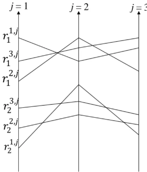
This condition avoids the overlapping of the reference profiles. Figure 1 shows three criteria, three decision-makers and three classes represented by two limiting profiles. In this case, the dominance condition is verified.
Figure 1. An example of Dominance condition respected
3.3. Comparison step
The comparison stage is based on the PROMETHEE algorithm (Brans & Vincke, 1985). Two alternatives 𝑎1and 𝑎2 are compared on a criterion 𝑔𝑗 by calculating the distance 𝑑𝑗(𝑎1, 𝑎2) =
𝑔𝑗(𝑎1) − 𝑔𝑗(𝑎2) in a uni-criterion preference degree 𝑃𝑗(𝑎1, 𝑎2), whose proprieties are: 0 ≤ 𝑃𝑗(𝑎1, 𝑎2) ≤ 1
𝑃𝑗(𝑎1, 𝑎2) ≈ 0 if 𝑎1 is indifferent to 𝑎2 on the criterion 𝑔𝑗
𝑃𝑗(𝑎1, 𝑎2) ≈ 1 if 𝑎1 is strictly preferred to 𝑎2 on the criterion 𝑔𝑗
Six different types of function 𝑃𝑗(𝑎1, 𝑎2), e.g. linear, step wise, Gaussian and so on, have been proposed (Brans & Vincke, 1985). They are defined by two shape parameters: preference and indifference threshold.
In Flow-Sort, each alternative 𝑎𝑖 ∈ 𝐴 is compared only to the reference profiles (Nemery & Lamboray, 2008). This technique is also used in Flow-Sort-GDSS but in using all references
𝑟11,𝑗
𝑟
12,𝑗 𝑟13,𝑗 𝑟23,𝑗 𝑟21,𝑗 𝑟22,𝑗 j= 1 j= 2 j= 38
profiles of all decision-makers. Therefore, the uni-criterion net flow of 𝑎𝑖 on criterion 𝑔𝑗 is defined as follows:
𝛷𝑗(𝑎𝑖) =|𝑅1𝑗|∑𝑟 [𝑃𝑗(𝑎𝑖, 𝑟𝑘𝑡,𝑗) − 𝑃𝑗(𝑟𝑘𝑡,𝑗, 𝑎𝑖)]
𝑘𝑡,𝑗∈𝑅𝑗 (1)
The net flow is between -1 and 1 depending on the strength (near 1) or the weakness (-1) of the alternative 𝑎𝑖relatively to the reference profiles on criterion 𝑔𝑗. Equation 1 is calculated with one alternative at the time for making 𝛷𝑗(𝑎𝑖) independent from the other alternatives of the set A.
The global net flow 𝛷(𝑎𝑖) is given by the weighted sum of the uni-criterion net flow:
𝛷(𝑎𝑖) = ∑𝐽𝑗=1𝑤𝑔𝑗𝛷𝑗(𝑎𝑖) (2)
where 𝑤𝑔𝑗represents the weight given to criterion j.
In order to situate the global net flow of the alternative 𝑎𝑖 regarding the reference profiles, the net flows of the 𝑇 × (𝐾 − 1) limiting profiles or 𝑇 × 𝐾 central profiles on the criterion 𝑔𝑗 have to be calculated. Therefore, the uni-criterion net flow of the reference profile 𝑟𝜅𝜏,𝑗 ∈𝑅𝑗 is compared in pairs with all reference profiles and the alternative 𝑎𝑖.
𝛷𝑗,𝑖(𝑟𝜅𝜏,𝑗) =|𝑅𝑗1|+1{∑ [𝑃𝑗(𝑟𝜅 𝜏,𝑗, 𝑟
𝑘𝑡,𝑗) − 𝑃𝑗(𝑟𝑘𝑡,𝑗, 𝑟𝜅𝜏,𝑗)]
𝑟𝑘𝑡,𝑗∈𝑅𝑗 + [ 𝑃𝑗(𝑟𝜅𝜏,𝑗, 𝑎𝑖) − 𝑃𝑗(𝑎𝑖, 𝑟𝜅𝜏,𝑗)]} (3)
The global net flow 𝛷𝑖(𝑟𝜅𝜏) referred to 𝑎𝑖 is given by the weighted sum of the uni-criterion net flow:
𝛷𝑖(𝑟𝜅𝜏) = ∑ 𝑤
𝑔𝑗𝛷𝑗,𝑖(𝑟𝜅 𝜏,𝑗) 𝐽
𝑗=1 (4)
Equations (1), (2), (3) and (4) are calculated for each 𝑎𝑖, i = 1, .., n.
Because of the dominance condition on the local classes (Section 3), it is proved that:
to the FMEA, Expert Systems with Applications, 42(17-18), 6342–6349
9
𝛷𝑖(𝑟𝑘𝑡) ≥ 𝛷
𝑖(𝑟𝑘+1𝑠 ); ∀ 𝑘 = 1, … , 𝐾 − 2 (limiting profiles) ˄ ∀ 𝑘 = 1, … , 𝐾 − 1 (central profiles),
∀ 𝑡, 𝑠 = 1, … , 𝑇 and ∀ 𝑖 = 1, … , 𝑛.
3.4. Assignment step
3.4.1.Introduction
The assignment procedure is composed of rules depending on the value of 𝛷(𝑎𝑖) (Equation (2)) with respect to the global net flows of the reference profiles (Equation (4)). These rules are explained in the sequel by distinguishing between the cases of limiting (section 3.4.2) or central profiles (section 3.4.3). In both cases, an assignment is ‘unanimous’ if all decision-makers agree with the assignment of the alternative to the same class. If the assignment is ‘non unanimous’, then the total distance between the global net flow of the alternative and the global net flows of the reference profiles is used. The lemma 1 of dominance on the global reference profiles (Section 3.3) always forces the divergence of assignment between decision-makers only between two consecutive classes at most.
3.4.2.Assignment with limiting profiles
Depending on the unanimousagreement or not of the decision-makers, two different assignment procedures are distinguished.
1. Unanimous assignment: Three cases exist:
a) If ∃ 𝑘, with 1 < 𝑘 < 𝐾 − 1, such that 𝛷𝑖(𝑟𝑘𝑡) ≥ 𝛷(𝑎𝑖) > 𝛷𝑖(𝑟𝑘+1𝑡 )∀𝑡 = 1, … , 𝑇 ⇒
𝐶(𝑎𝑖) = 𝐶𝑘
b) If 𝛷(𝑎𝑖) ≥ 𝛷𝑖(𝑟1𝑡), ∀𝑡 = 1, … , 𝑇 ⇒ 𝐶(𝑎𝑖) = 𝐶1
c) If 𝛷(𝑎𝑖) < 𝛷𝑖(𝑟𝐾−1𝑡 ), ∀𝑡 = 1, … , 𝑇 ⇒ 𝐶(𝑎𝑖) = 𝐶𝐾
The assignment rules b) and c) are for the highest and lowest class, respectively. The assignment rule a) is for all the other classes.
2. Non unanimous assignment.
If at least two decision-makers t and s exist such that𝛷𝑖(𝑟𝑘𝑡) ≤ 𝛷(𝑎𝑖) < 𝛷𝑖(𝑟𝑘𝑠), which means that 𝑡 and 𝑠 assign 𝑎𝑖 respectively to 𝐶𝑘 and 𝐶𝑘+1.
10
The non unanimous assignment consists of two subsequent steps:
i. The distances 𝑑𝑖(𝑘) and 𝑑𝑖(𝑘 + 1) between the net flow 𝛷(𝑎𝑖) and the net flows of the global limiting profiles of the decision-makers assigning 𝑎𝑖 to 𝐶𝑘 and 𝐶𝑘+1are
calculated as follows (in respective order):-
𝑑𝑖(𝑘) = ∑𝑡:𝛷(𝑎𝑖)≥𝛷𝑖(𝑟𝑘𝑡)𝑤𝑑𝑡[𝛷(𝑎𝑖) − 𝛷(𝑟𝑘𝑡)] (5)
𝑑𝑖(𝑘 + 1) = ∑𝑠:𝛷(𝑎𝑖)<𝛷𝑖(𝑟𝑘𝑠)𝑤𝑑𝑠[𝛷(𝑟𝑘+1𝑠 ) − 𝛷(𝑎𝑖)] (6)
where 𝑤𝑑𝑡 and 𝑤𝑑𝑠 are the weights respectively given to the decision-makers 𝑡 and 𝑠, which represents the experience and knowledge of the decision-maker involved in the sorting process. Thereby, Equation (5) and (6) provide the weighted average distances between 𝛷(𝑎𝑖) and the global limiting profiles of their respective classes. This
represents a degree of membership to 𝐶𝑘 and 𝐶𝑘+1.
ii. The distances 𝑑𝑖(𝑘) and 𝑑𝑖(𝑘 + 1) are compared in order to conclude the class
assignment on the basis of the degree of membership to 𝐶𝑘 and 𝐶𝑘+1. The smallest the distance to the limiting profile defines the class. In case of equal distance, two
assignments are possible according to the vision of the decision-makers. In an optimistic vision, the alternative is assigned to the higher class and in a pessimistic vision it is assigned to the lower class. The three assignment rules are defined as following:
a) If 𝑑𝑖(𝑘 + 1) − 𝑑𝑖(𝑘) > 0 ⇒ 𝐶(𝑎𝑖) = 𝐶𝑘
b) If 𝑑𝑖(𝑘 + 1) − 𝑑𝑖(𝑘) < 0 ⇒ 𝐶(𝑎𝑖) = 𝐶𝑘+1
c) If 𝑑𝑖(𝑘 + 1) − 𝑑𝑖(𝑘) = 0⇒ in an optimistic vision 𝐶(𝑎𝑖) = 𝐶𝑘 in a pessimistic vision 𝐶(𝑎𝑖) = 𝐶𝑘+1.
3.4.3.Assignment with central profiles
Depending on the unanimousagreement or not of the decision-makers, two different assignment procedures are distinguished.
to the FMEA, Expert Systems with Applications, 42(17-18), 6342–6349
11
1. Unanimous assignment.
If all T global central profiles of class Ck are the closest to the global net flow of 𝑎𝑖,then all
decision-makers agree with the assignment of 𝑎𝑖 to 𝐶𝑘.
If ∃ 𝑘, with 1 ≤ 𝑘 ≤ 𝐾, 𝑠𝑢𝑐ℎ 𝑡ℎ𝑎𝑡 |𝛷𝑖(𝑟𝑘𝑡) − 𝛷(𝑎𝑖)| < |𝛷𝑖(𝑟ℎ𝑡) − 𝛷(𝑎𝑖)|,∀𝑡 = 1, … , 𝑇 and
∀ℎ = 1, … , 𝐾\{ℎ} ⇒ 𝐶(𝑎𝑖) = 𝐶𝑘. 2. Non unanimous assignment.
If at least two decision-makers (t and s) and two different classes (k and h) exist such that
|𝛷𝑖(𝑟𝑘𝑡) − 𝛷(𝑎𝑖)| ≤ |𝛷𝑖(𝑟ℎ𝑡) − 𝛷(𝑎𝑖)|∀ℎ = 1, … , 𝐾 and |𝛷𝑖(𝑟𝑘𝑠) − 𝛷(𝑎𝑖)| ≥ |𝛷𝑖(𝑟ℎ𝑠) −
𝛷(𝑎𝑖)|∀𝑘 = 1, … , 𝐾, it means that 𝑡 and 𝑠 assign 𝑎𝑖 respectively to 𝐶𝑘 and 𝐶ℎor have an equal preference for 𝐶𝑘 and 𝐶ℎ in case of an equality sign. It is to remark that the lemma of the dominance (Section 3.3) leads to ℎ = 𝑘 ± 1. Thereby, without loss of generality, in order to simplify the notation let be 𝑇𝑘 and 𝑇𝑘+1 the set of decision-makers assigning 𝑎𝑖 respectively to 𝐶𝑘 and 𝐶𝑘+1.
As in the case of the limiting profiles, the non unanimous assignment has two steps: i. The distances di(k) and di(k+1) between the net flow 𝛷(𝑎𝑖) and the net flows of the
central profiles defined by the decision-makers assigning 𝑎𝑖 to 𝐶𝑘 and 𝐶𝑘+1are respectively calculated as follows:
𝑑𝑖(𝑘) = ∑𝑡∈𝑇𝑘𝑤𝑑𝑡· |𝛷𝑖(𝑟𝑘𝑡) − 𝛷(𝑎𝑖)| (7)
𝑑𝑖(𝑘 + 1) = ∑ 𝑤𝑑𝑠· |𝛷𝑖(𝑟𝑘+1𝑠 ) − 𝛷(𝑎 𝑖)|
𝑠∈𝑇𝑘+1 (8)
where 𝑤𝑑𝑡 and 𝑤𝑑𝑠 are the weights respectively given to the decision-makers 𝑡 and 𝑠. Equations 7 and 8 provide the weighted distances between 𝛷(𝑎𝑖) and the global central profiles of their respective classes. They represent respectively the degree of
membership to 𝐶𝑘 and 𝐶𝑘+1.
ii. The distances 𝑑𝑖(𝑘) and 𝑑𝑖(𝑘 + 1) are compared in order to conclude the class
assignment on the basis of the degree of membership to 𝐶𝑘 and 𝐶𝑘+1. The smallest the distance to the limiting profile defines the class. In case of equal distance, two
assignments are possible according to the vision of the decision-makers. In an optimistic vision, the alternative is assigned to the higher class and in a pessimistic vision it is assigned to the lower class. The three assignment rules are defined as following:
12 a) If 𝑑𝑖(𝑘 + 1) − 𝑑𝑖(𝑘) > 0 ⇒ 𝐶(𝑎𝑖) = 𝐶𝑘
b) If 𝑑𝑖(𝑘 + 1) − 𝑑𝑖(𝑘) < 0 ⇒ 𝐶(𝑎𝑖) = 𝐶𝑘+1
c) If 𝑑𝑖(𝑘 + 1) − 𝑑𝑖(𝑘) = 0
4. Case study
This section presents the application of FlowSort-GDSS to the FMEA on plastic bottles
manufacturing, through a blow-moulding process. Some features of the operative environment have to be clarified before showing the numerical illustration. When the FMEA is applied to the plastic bottles (i.e. the final products of a blow-moulding process) of an already existing process, failure modes regard the defects occurred in a pre-defined time horizon to the bottles, e.g. oval neck, weak handle welding, and so on. They in turn should be correlated to their causes related to machines and/or technological process. However, as often happens in real industrial contexts, the failure causes are not directly traceable when the failure modes are reported by inline operators without any specific knowledge on the process. In this case, the FMEA is applied to the failure modes of the final products, and FlowSort-GDSS is used for classifying them into priority classes.
4.1. FlowSort-GDSS:
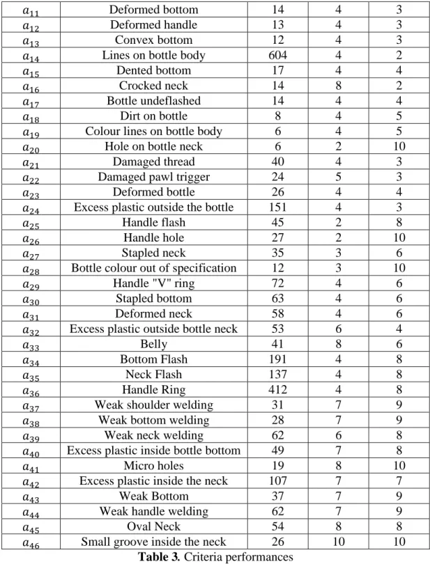
A large dataset consisting of 2673 events of 46 different failure modes (i.e. alternatives with 𝑛 =
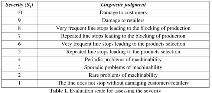
46) is registered during one year by visual inspections performed by inline operators. The product, quality and process managers have then agreed on the severity (S) of the failures by using Table 1 and on the detectability (D) by using Table 2. The occurrence (O) is simply given by the number of observed events. Table 3 reports these values for all the alternatives denoted by 𝑎𝑖, with 𝑖 =
1, … ,46. The objective of the application of the FlowSort-GDSS to these 46 failures is thus to sort them into 3 priority classes (𝐾 = 3).
to the FMEA, Expert Systems with Applications, 42(17-18), 6342–6349
13
Severity (𝑺𝒊) Linguistic judgment
10 Damage to customers
9 Damage to retailers
8 Very frequent line stops leading to the blocking of production 7 Repeated line stops leading to the blocking of production 6 Very frequent line stops leading to the products selection 5 Repeated line stops leading to the products selection
4 Periodic problems of machinability
3 Sporadic problems of machinability
2 Rare problems of machinability
1 The line does not stop without damaging customers/retailers
Table 1.Evaluation scale for assessing the severity
Detectability
(𝑫𝒊) Linguistic judgment
10 No identifying test
9 A visual test exists and a highly skilled technician can perform it using dedicated tools
8 A visual test exists and expert highly skilled technician can perform it 7 A visual test exists and a fairly skilled operator can perform it using
dedicated tools
6 A visual test exists and a fairly skilled operator can perform it 5 A visual test exists and it’s easy to identify the failure using dedicated tools 4 A visual test exists and it’s easy to identify the failure
3 A visual test exists and the failure is immediately found using dedicated tools (water test)
2 A visual test exists and the failure is immediately found
1 Automatic test
Table 2.Evaluation scale for assessing the detectability
𝒂𝒊 Failure Oi Di Si
𝑎1 Low weight 2 2 1
𝑎2 High weight 10 2 1
𝑎3 Irregular surface on bottle body 3 4 1
𝑎4 Weak handle 2 4 2
𝑎5 Hole on bottle bottom 2 2 10
𝑎6 Black spots on bottle body 15 5 1
𝑎7 Neck height out of specification 15 2 4
𝑎8 Hole on bottle shoulder 3 2 10
𝑎9 Weak bottle shoulder 42 3 2
14
𝑎11 Deformed bottom 14 4 3
𝑎12 Deformed handle 13 4 3
𝑎13 Convex bottom 12 4 3
𝑎14 Lines on bottle body 604 4 2
𝑎15 Dented bottom 17 4 4
𝑎16 Crocked neck 14 8 2
𝑎17 Bottle undeflashed 14 4 4
𝑎18 Dirt on bottle 8 4 5
𝑎19 Colour lines on bottle body 6 4 5
𝑎20 Hole on bottle neck 6 2 10
𝑎21 Damaged thread 40 4 3
𝑎22 Damaged pawl trigger 24 5 3
𝑎23 Deformed bottle 26 4 4
𝑎24 Excess plastic outside the bottle 151 4 3
𝑎25 Handle flash 45 2 8
𝑎26 Handle hole 27 2 10
𝑎27 Stapled neck 35 3 6
𝑎28 Bottle colour out of specification 12 3 10
𝑎29 Handle "V" ring 72 4 6
𝑎30 Stapled bottom 63 4 6
𝑎31 Deformed neck 58 4 6
𝑎32 Excess plastic outside bottle neck 53 6 4
𝑎33 Belly 41 8 6
𝑎34 Bottom Flash 191 4 8
𝑎35 Neck Flash 137 4 8
𝑎36 Handle Ring 412 4 8
𝑎37 Weak shoulder welding 31 7 9
𝑎38 Weak bottom welding 28 7 9
𝑎39 Weak neck welding 62 6 8
𝑎40 Excess plastic inside bottle bottom 49 7 8
𝑎41 Micro holes 19 8 10
𝑎42 Excess plastic inside the neck 107 7 7
𝑎43 Weak Bottom 37 7 9
𝑎44 Weak handle welding 62 7 9
𝑎45 Oval Neck 54 8 8
𝑎46 Small groove inside the neck 26 10 10
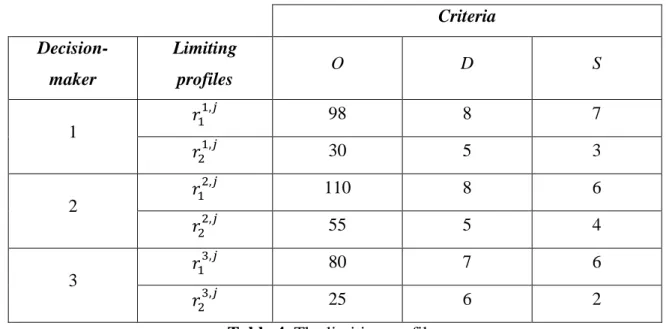
Table 3.Criteria performances Each manager characterises the classes with a limiting profile (Table 4).
to the FMEA, Expert Systems with Applications, 42(17-18), 6342–6349 15 Criteria Decision-maker Limiting profiles O D S 1 𝑟11,𝑗 98 8 7 𝑟21,𝑗 30 5 3 2 𝑟12,𝑗 110 8 6 𝑟22,𝑗 55 5 4 3 𝑟13,𝑗 80 7 6 𝑟23,𝑗 25 6 2
Table 4. The limiting profiles
As the decision-makers have the same importance, the same weight 𝑤𝑑 is allocated to them.
4.2. Flowsort-GDSS: comparison step
For the pair-wise comparison, the linear preference function 𝑃𝑗(𝑎1, 𝑎2) is selected for each criterion j. The indifference and preference thresholds are given in Table 5.
O D S
Indifference
threshold 0 0 0
Preference
threshold 602 8 9
Table 5.The preference thresholds.
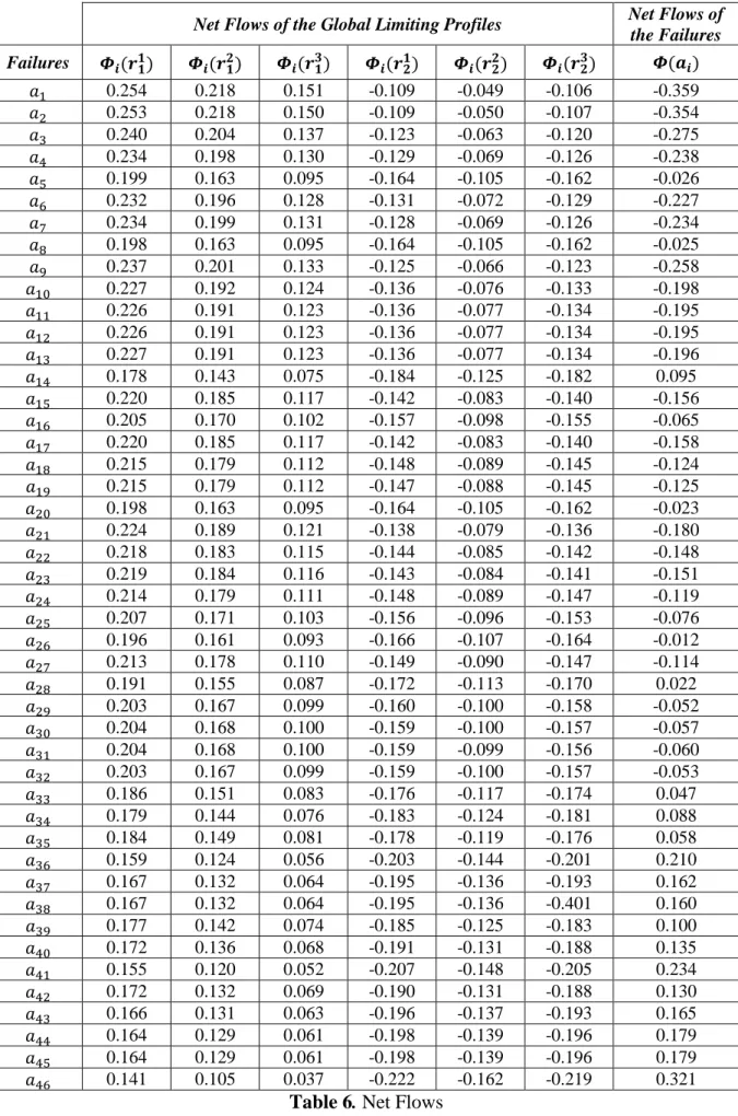
The software Smart-Picker is then used to calculated the net flow of the global limiting profiles
𝛷𝑖(𝑟𝑘𝑡), with 𝑘 = 1,2, 𝑡 = 1,2,3 and 𝑖 = 1, … ,46 and the net flow of the failures 𝛷(𝑎
𝑖), with
16
Net Flows of the Global Limiting Profiles Net Flows of
the Failures Failures 𝜱𝒊(𝒓𝟏𝟏) 𝜱𝒊(𝒓𝟏𝟐) 𝜱𝒊(𝒓𝟏𝟑) 𝜱𝒊(𝒓𝟐𝟏) 𝜱𝒊(𝒓𝟐𝟐) 𝜱𝒊(𝒓𝟐𝟑) 𝜱(𝒂𝒊) 𝑎1 0.254 0.218 0.151 -0.109 -0.049 -0.106 -0.359 𝑎2 0.253 0.218 0.150 -0.109 -0.050 -0.107 -0.354 𝑎3 0.240 0.204 0.137 -0.123 -0.063 -0.120 -0.275 𝑎4 0.234 0.198 0.130 -0.129 -0.069 -0.126 -0.238 𝑎5 0.199 0.163 0.095 -0.164 -0.105 -0.162 -0.026 𝑎6 0.232 0.196 0.128 -0.131 -0.072 -0.129 -0.227 𝑎7 0.234 0.199 0.131 -0.128 -0.069 -0.126 -0.234 𝑎8 0.198 0.163 0.095 -0.164 -0.105 -0.162 -0.025 𝑎9 0.237 0.201 0.133 -0.125 -0.066 -0.123 -0.258 𝑎10 0.227 0.192 0.124 -0.136 -0.076 -0.133 -0.198 𝑎11 0.226 0.191 0.123 -0.136 -0.077 -0.134 -0.195 𝑎12 0.226 0.191 0.123 -0.136 -0.077 -0.134 -0.195 𝑎13 0.227 0.191 0.123 -0.136 -0.077 -0.134 -0.196 𝑎14 0.178 0.143 0.075 -0.184 -0.125 -0.182 0.095 𝑎15 0.220 0.185 0.117 -0.142 -0.083 -0.140 -0.156 𝑎16 0.205 0.170 0.102 -0.157 -0.098 -0.155 -0.065 𝑎17 0.220 0.185 0.117 -0.142 -0.083 -0.140 -0.158 𝑎18 0.215 0.179 0.112 -0.148 -0.089 -0.145 -0.124 𝑎19 0.215 0.179 0.112 -0.147 -0.088 -0.145 -0.125 𝑎20 0.198 0.163 0.095 -0.164 -0.105 -0.162 -0.023 𝑎21 0.224 0.189 0.121 -0.138 -0.079 -0.136 -0.180 𝑎22 0.218 0.183 0.115 -0.144 -0.085 -0.142 -0.148 𝑎23 0.219 0.184 0.116 -0.143 -0.084 -0.141 -0.151 𝑎24 0.214 0.179 0.111 -0.148 -0.089 -0.147 -0.119 𝑎25 0.207 0.171 0.103 -0.156 -0.096 -0.153 -0.076 𝑎26 0.196 0.161 0.093 -0.166 -0.107 -0.164 -0.012 𝑎27 0.213 0.178 0.110 -0.149 -0.090 -0.147 -0.114 𝑎28 0.191 0.155 0.087 -0.172 -0.113 -0.170 0.022 𝑎29 0.203 0.167 0.099 -0.160 -0.100 -0.158 -0.052 𝑎30 0.204 0.168 0.100 -0.159 -0.100 -0.157 -0.057 𝑎31 0.204 0.168 0.100 -0.159 -0.099 -0.156 -0.060 𝑎32 0.203 0.167 0.099 -0.159 -0.100 -0.157 -0.053 𝑎33 0.186 0.151 0.083 -0.176 -0.117 -0.174 0.047 𝑎34 0.179 0.144 0.076 -0.183 -0.124 -0.181 0.088 𝑎35 0.184 0.149 0.081 -0.178 -0.119 -0.176 0.058 𝑎36 0.159 0.124 0.056 -0.203 -0.144 -0.201 0.210 𝑎37 0.167 0.132 0.064 -0.195 -0.136 -0.193 0.162 𝑎38 0.167 0.132 0.064 -0.195 -0.136 -0.401 0.160 𝑎39 0.177 0.142 0.074 -0.185 -0.125 -0.183 0.100 𝑎40 0.172 0.136 0.068 -0.191 -0.131 -0.188 0.135 𝑎41 0.155 0.120 0.052 -0.207 -0.148 -0.205 0.234 𝑎42 0.172 0.132 0.069 -0.190 -0.131 -0.188 0.130 𝑎43 0.166 0.131 0.063 -0.196 -0.137 -0.193 0.165 𝑎44 0.164 0.129 0.061 -0.198 -0.139 -0.196 0.179 𝑎45 0.164 0.129 0.061 -0.198 -0.139 -0.196 0.179 𝑎46 0.141 0.105 0.037 -0.222 -0.162 -0.219 0.321
to the FMEA, Expert Systems with Applications, 42(17-18), 6342–6349
17
4.3. Flowsort-GDSS: assignment step
The assignment rules described in section 3.4 are applied on the net flows of
Net Flows of the Global Limiting Profiles Net Flows of
the Failures Failures 𝜱𝒊(𝒓𝟏𝟏) 𝜱𝒊(𝒓𝟏𝟐) 𝜱𝒊(𝒓𝟏𝟑) 𝜱𝒊(𝒓𝟐𝟏) 𝜱𝒊(𝒓𝟐𝟐) 𝜱𝒊(𝒓𝟐𝟑) 𝜱(𝒂𝒊) 𝑎1 0.254 0.218 0.151 -0.109 -0.049 -0.106 -0.359 𝑎2 0.253 0.218 0.150 -0.109 -0.050 -0.107 -0.354 𝑎3 0.240 0.204 0.137 -0.123 -0.063 -0.120 -0.275 𝑎4 0.234 0.198 0.130 -0.129 -0.069 -0.126 -0.238 𝑎5 0.199 0.163 0.095 -0.164 -0.105 -0.162 -0.026 𝑎6 0.232 0.196 0.128 -0.131 -0.072 -0.129 -0.227 𝑎7 0.234 0.199 0.131 -0.128 -0.069 -0.126 -0.234 𝑎8 0.198 0.163 0.095 -0.164 -0.105 -0.162 -0.025 𝑎9 0.237 0.201 0.133 -0.125 -0.066 -0.123 -0.258 𝑎10 0.227 0.192 0.124 -0.136 -0.076 -0.133 -0.198 𝑎11 0.226 0.191 0.123 -0.136 -0.077 -0.134 -0.195 𝑎12 0.226 0.191 0.123 -0.136 -0.077 -0.134 -0.195 𝑎13 0.227 0.191 0.123 -0.136 -0.077 -0.134 -0.196 𝑎14 0.178 0.143 0.075 -0.184 -0.125 -0.182 0.095 𝑎15 0.220 0.185 0.117 -0.142 -0.083 -0.140 -0.156 𝑎16 0.205 0.170 0.102 -0.157 -0.098 -0.155 -0.065 𝑎17 0.220 0.185 0.117 -0.142 -0.083 -0.140 -0.158 𝑎18 0.215 0.179 0.112 -0.148 -0.089 -0.145 -0.124 𝑎19 0.215 0.179 0.112 -0.147 -0.088 -0.145 -0.125 𝑎20 0.198 0.163 0.095 -0.164 -0.105 -0.162 -0.023 𝑎21 0.224 0.189 0.121 -0.138 -0.079 -0.136 -0.180 𝑎22 0.218 0.183 0.115 -0.144 -0.085 -0.142 -0.148 𝑎23 0.219 0.184 0.116 -0.143 -0.084 -0.141 -0.151 𝑎24 0.214 0.179 0.111 -0.148 -0.089 -0.147 -0.119 𝑎25 0.207 0.171 0.103 -0.156 -0.096 -0.153 -0.076 𝑎26 0.196 0.161 0.093 -0.166 -0.107 -0.164 -0.012 𝑎27 0.213 0.178 0.110 -0.149 -0.090 -0.147 -0.114 𝑎28 0.191 0.155 0.087 -0.172 -0.113 -0.170 0.022 𝑎29 0.203 0.167 0.099 -0.160 -0.100 -0.158 -0.052 𝑎30 0.204 0.168 0.100 -0.159 -0.100 -0.157 -0.057 𝑎31 0.204 0.168 0.100 -0.159 -0.099 -0.156 -0.060 𝑎32 0.203 0.167 0.099 -0.159 -0.100 -0.157 -0.053 𝑎33 0.186 0.151 0.083 -0.176 -0.117 -0.174 0.047 𝑎34 0.179 0.144 0.076 -0.183 -0.124 -0.181 0.088 𝑎35 0.184 0.149 0.081 -0.178 -0.119 -0.176 0.058 𝑎36 0.159 0.124 0.056 -0.203 -0.144 -0.201 0.210 𝑎37 0.167 0.132 0.064 -0.195 -0.136 -0.193 0.162 𝑎38 0.167 0.132 0.064 -0.195 -0.136 -0.401 0.160 𝑎39 0.177 0.142 0.074 -0.185 -0.125 -0.183 0.100 𝑎40 0.172 0.136 0.068 -0.191 -0.131 -0.188 0.135 𝑎41 0.155 0.120 0.052 -0.207 -0.148 -0.205 0.234
18 𝑎42 0.172 0.132 0.069 -0.190 -0.131 -0.188 0.130 𝑎43 0.166 0.131 0.063 -0.196 -0.137 -0.193 0.165 𝑎44 0.164 0.129 0.061 -0.198 -0.139 -0.196 0.179 𝑎45 0.164 0.129 0.061 -0.198 -0.139 -0.196 0.179 𝑎46 0.141 0.105 0.037 -0.222 -0.162 -0.219 0.321
Table 6. Some examples illustrating the assignment procedure are described in the following: For the unanimous assignment:
Failure 𝑎8 is assigned to 𝐶2 because a class exists (𝐶2) such that its global net flow (-0.025) lies between the global net flows of all the limiting profiles of the classes 𝐶1 and 𝐶3
(Condition (a) of Section 4.2).
Failure 𝑎45 is assigned to 𝐶1 because its global net flow (0.179) is greater than or equal to all the global net flows of the limiting profiles of the class 𝐶1 (Condition (b) of Section 4.2). Failure 𝑎1 is assigned to 𝐶3 because its global net flow (-0.359) is less than all the global net
flows of the limiting profiles of the class 𝐶3 (Condition (c) of Section 4.2).
The non unanimous assignment is performed whenever at least two decision-makers would assign the alternative to different classes. For instance, the assignment of failure 𝑎27 is non unanimous because decision-makers 1 and 3 would assign it to 𝐶2 (−0.114 ≥ −0.149 𝑎𝑛𝑑 − 0.114 ≥
−0.147), whilst decision-maker 2 to 𝐶3 (−0.114 < −0.090). Thereby, Equation 5 and 6 have to be respectively applied to decision-makers 1 and 3 and to decision-maker 2, where the decision-makers are equally weighted (i.e. 0.33). They respectively provide these values: 𝑑27(2) = (0.33 ∗
0.035) + (0.33 ∗ 0.033) = 0.02264; 𝑑27(3) = 0.33 ∗ 0.024 = 0.00799. Since 0.02264 −
0.00799 > 0, then 𝑎5 is assigned to 𝐶2 (Condition (d) of Section 4.2).
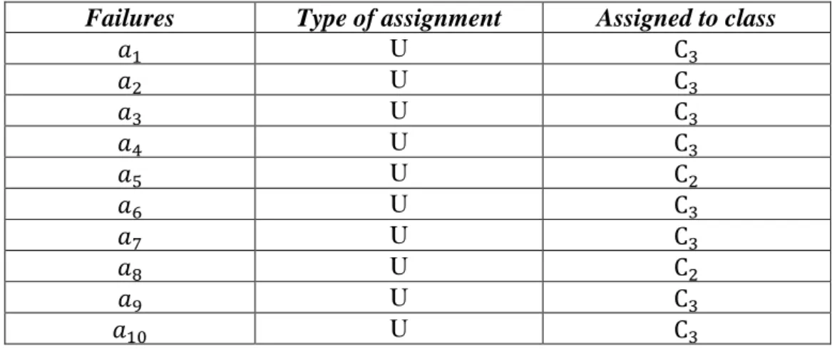
Table 9 reports the final sorting either by unanimous (“U” in 2th column) or non unanimous assignments (“NU” in the 2th column).
Failures Type of assignment Assigned to class
𝑎1 U C3 𝑎2 U C3 𝑎3 U C3 𝑎4 U C3 𝑎5 U C2 𝑎6 U C3 𝑎7 U C3 𝑎8 U C2 𝑎9 U C3 𝑎10 U C3
to the FMEA, Expert Systems with Applications, 42(17-18), 6342–6349 19 𝑎11 U C3 𝑎12 U C3 𝑎13 U C3 𝑎14 NU C2 𝑎15 U C3 𝑎16 U C2 𝑎17 U C3 𝑎18 NU C2 𝑎19 NU C2 𝑎20 U C2 𝑎21 U C3 𝑎22 U C3 𝑎23 U C3 𝑎24 NU C2 𝑎25 U C2 𝑎26 U C2 𝑎27 NU C2 𝑎28 U C2 𝑎29 U C2 𝑎30 U C2 𝑎31 U C2 𝑎32 U C2 𝑎33 U C2 𝑎34 NU C2 𝑎35 U C2 𝑎36 U C1 𝑎37 NU C1 𝑎38 NU C1 𝑎39 NU C2 𝑎40 NU C1 𝑎41 U C1 𝑎42 NU C1 𝑎43 NU C1 𝑎44 U C1 𝑎45 U C1 𝑎46 U C1
Table 7.Sorting of the failures with Flowsort-GDSS.
In this case study, ten failures are 𝐶1 classified and thus prioritised for improvement interventions. As shown in Table 7, twelve non unanimous assignments exist. In these cases, decision-makers would remain in a conflicting state without such a group decision support system. FlowSort-GDSS reveals its strength exactly when an individual sorting method fails.
20
5. Conclusion
FMEA is recognised in industrial settings as an operative tool for quality improvement of both the products and the processes. Although several shortcomings of the traditional FMEA have already been addressed, we have seen that some of them are still unsolved. The ranking of the failure modes does not directly provide clear classes of risk levels. In particular, when dealing with a large number of failure modes, classifying them into priority classes by an expert and intelligent system allows managers to be focused on the most critical ones. Therefore, this qualifies to be a multi-criteria sorting problem. Furthermore, the FMEA generally involves several decision-makers with different experiences and skills. However, literature lacks of contributions on expert and intelligent group decisions systems, especially for the FMEA. In this paper, a novel MCDM approach named
FlowSort-GDSS has been introduced for facing such a group decision sorting issue. It requires that the decision-makers establish the reference profiles on each risk factor for defining each priority class. Thereby, the global classification of the failure modes incorporate multitude of experiences and several points of view coming from multiple decision-makers.
FlowSort-GDSS incorporates the generic advantages of the MCDM methods, which are able to overcome the standard FMEA shortcomings (e.g. different degree of importance may be assigned to the risk factors, construction of a risk function) and the specific advantages of the outranking
methods: it does not require any normalisation. This addresses the problem of the choice of the normalisation method which may lead to different outcomes. As a consequence, the classification does not depend on the failure modes stored into the dataset. This feature represents a relevant advantage in real settings, when FMEA is periodically reviewed and new types of failure modes eventually appear into the dataset. In fact, the already classified failure modes will not change their priority classes because they are only compared to the same reference profile. Moreover, FlowSort-GDSS avoids compensatory effects. A low score on one risk factor cannot be compensated by a high score on another risk factor and therefore problems cannot be hidden and ignored.
Furthermore, FlowSort-GDSS is highly flexible, that is it can be customised by adopting different preference (risk) functions, as well as by assigning different weights to the decision-makers.
The practical advantages of FlowSort-GDSS have been confirmed in the industrial case study of the blow moulding process, where a large dataset of product failures have been collected. Sorting these failures into priority classes allowed the company to focus the improvement actions only on the
to the FMEA, Expert Systems with Applications, 42(17-18), 6342–6349
21
most critical ones. It is worth to remark that FlowSort-GDSS is generic enough to be used in other sorting problems involving several decision-makers.
It is to note that the advanced information provided by FlowSort-GDSS also require more inputs from the decision-makers, which can be time-consuming. Other limitations of FlowSort-GDSS exists and they require further research. The economical dimension is not taken into account. This is an important further research direction because budget are often limited. Moreover, the
improvements are not necessarily linear correlated with the investments, which means that a non-linear optimisation problem needs to be solved. The FMEA has been considered as a snapshot of the quality production. This does not take into account that the different improvement and degradation rate over time. FMEA could benefit from continuous improvement theory by
introducing quality-based learning curves. It is also to note that we have assumed that the failures are independent. This is not always the case, for example one improvement action can solve several failures. Therefore, further research would be to take into account the interdependent failures while building the model.
Acknowledgment
The authors wish to thank Sajid Siraj for his proofreading.
References
Bozdag, E., Asan, U., Soyer, A., & Serdarasan, S. (2015). Risk prioritization in Failure Mode and Effects Analysis using interval type-2 fuzzy sets. Expert Systems with Applications, 42, 4000–4015.
Braglia, M. (2000). MAFMA: multi‐attribute failure mode analysis. International Journal of Quality & Reliability Management, 17, 1017 - 1033.
Braglia, M., Frosolini, M., & Montanari, R. (2003). Fuzzy TOPSIS approach for failure mode, effects and criticality analysis. Quality and Reliability Engineering International, 19, 425-443.
Brans, J.-P., & Vincke, P. (1985). A preference ranking organisation method. Management Science, 31, 647-656.
Carmignani, G. (2009). An integrated structural framework to cost-based FMECA: The priority-cost FMECA. Reliability Engineering and System Safety, 94, 861-871.
22
Chang, C., Liu, P., & Wei, C. (2001). Failure mode and effects analysis using grey theory. Integrated Manufacturing Systems, 12, 211 - 216.
Chang, C., Wei, C., & Lee, Y. (1999). Failure mode and effects analysis using fuzzy method and grey theory. Kybernetes, 28, 1072-1080.
Chang, D., & Sun, K.-L. (2009). Applying DEA to enhance assessment capability of FMEA. International Journal of Quality & Reliability Management, 26, 629 - 643.
Chang, K.-H. (2009). Evaluate the orderings of risk for failure problems using a more general RPN methodology. Microelectronics Reliability, 49, 1586-1596.
Chang, K.-H., & Cheng, C.-H. (2011). Evaluating the risk of failure using the fuzzy OWA and DEMATEL method. Journal of Intelligent Manufacturing, 22, 113-129.
Chang, K., & Wen, T. (2010). A novel efficient approach for DFMEA combining 2-tuple and the OWA operator. Expert Systems with Applications, 37, 2362-2370.
Chin, K., Wang, Y., Poon, G., & Yang, J.-B. (2009). Failure mode and effects analysis by data envelopment analysis. Decision Support Systems, 48, 246-256.
Chin, K., Wang, Y., Poon, G., & Yang, J. (2009). Failure mode and effects analysis using a group-based evidential reasoning approach. Computers & Operations Research, 36, 1768-1779. Deng, X., Hu, Y., Deng, Y., & Mahadevan, S. (2014a). Environmental impact assessment based on
D numbers. Expert Systems with Applications, 41, 635–643.
Deng, X., Hu, Y., Deng, Y., & Mahadevan, S. (2014b). Supplier selection using AHP methodology extended by D numbers. Expert Systems with Applications, 41, 156–167.
Garcia, P., Schirru, R., & Frutoso e Melo, P. (2005). A fuzzy data envelopment analysis approach for FMEA. Progress in Nuclear Energy, 46, 359-373.
Hadi-Vencheh, A., & Aghajani, M. (2013). Failure mode and effects analysis A fuzzy group MCDM approach. Journal of Soft Computing and Applications, 2013, 1-14.
Hu, A., Hsu, C.-W., Kuo, T.-C., & Wu, W.-C. (2009). Risk evaluation of green components to hazardous substance using FMEA and FAHP. Expert Systems with Applications, 36, 7142-7147.
Ishizaka, A., & Nemery, P. (2011). Selecting the best statistical distribution with PROMETHEE and GAIA. Computers & Industrial Engineering, 61, 958-969.
Ishizaka, A., & Nguyen, N. (2013). Calibrated fuzzy AHP for current bank account selection. Expert Systems with Applications, 40, 3775-3783.
Kutlu, A., & Ekmekçioğlu, M. (2012). Fuzzy failure modes and effects analysis by using fuzzy TOPSIS-based fuzzy AHP. Expert Systems with Applications, 39, 61-67.
to the FMEA, Expert Systems with Applications, 42(17-18), 6342–6349
23
Liu, H.-C., Liu, L., Bian, Q.-H., Lin, Q.-L., Dong, N., & Xu, P.-C. (2011). Failure mode and effects analysis using fuzzy evidential reasoning approach and grey theory. Expert Systems with Applications, 38, 4403-4415.
Liu, H.-C., Liu, L., & Liu, N. (2013). Risk evaluation approaches in failure mode and effects analysis: A literature review. Expert Systems with Applications, 40, 828-838.
Liu, H.-C., Liu, L., Liu, N., & Mao, L.-X. (2012). Risk evaluation in failure mode and effects analysis with extended VIKOR method under fuzzy environment. Expert Systems with Applications, 39, 12926-12934.
Liu, H.-C., You, J.-X., Fan, X.-J., & Lin, Q.-L. (2014). Failure mode and effects analysis using D numbers and grey relational projection method. Expert Systems with Applications, 41, 4670-4679.
Mandal, S., & Maiti, J. (2014). Risk analysis using FMEA: Fuzzy similarity value and possibility theory based approach. Expert Systems with Applications, 41, 3527-3537.
Mardani, A., Jusoh, A., & Zavadskas, E. (2015). Fuzzy multiple criteria decision-making
techniques and applications – Two decades review from 1994 to 2014. Expert Systems with Applications, 42, 4126–4148.
Nemery, P. (2008). Extensions of the FlowSort sorting method for group decision-making. In 19th International Conference on Multiple Criteria Decision Making. Auckland.
Nemery, P., & Lamboray, C. (2008). FlowSort: a flow-based sorting method with limiting or central profiles. TOP, 16, 90-113.
Netto, T., Honorato, H., & Qassim, R. (2013). Prioritization of failure risk in subsea flexible pipes via data envelopment analysis. Marine Structures, 34, 105-116.
Petrović, D., Tanasijević, M., Milić, V., Lilić, N., Stojadinović, S., & Svrkota, I. (2014). Risk assessment model of mining equipment failure based on fuzzy logic. Expert Systems with Applications, 41, 8157-8164.
Seyed-Hosseini, S., Safaei, N., & Asgharpour, M. (2006). Reprioritization of failures in a system failure mode and effects analysis by decision making trial and evaluation laboratory technique. Reliability Engineering & System Safety, 91, 872–881.
Vahdani, B., Salimi, M., & Charkhchian, M. (2015). A new FMEA method by integrating fuzzy belief structure and TOPSIS to improve risk evaluation process. The International Journal of Advanced Manufacturing Technology, 77, 357-368.
24
Wang, Y.-M., Chin, K.-S., Poon, G., & Yang, J.-B. (2009). Risk evaluation in failure mode and effects analysis using fuzzy weighted geometric mean. Expert Systems with Applications, 36, 1195-1207.
Zammori, F., & Gabbrielli, R. (2012). ANP/RPN: a multi criteria evaluation of the Risk Priority Number. Quality and Reliability Engineering International, 28, 85-104.
Zhang, Z., & Chu, X. (2011). Risk prioritization in failure mode and effects analysis under uncertainty. Expert Systems with Applications, 38, 206-214.
View publication stats View publication stats