The Interaction of the IFRS 9 Expected Loss Approach with Supervisory
Rules and Implications for Financial Stability
Zoltán Novotny-Farkas
Lancaster University Management School Lancaster University
Lancaster LA1 4YX, UK
June 2016
Accounting in Europe (forthcoming)
Correspondence Address: Zoltán Novotny-Farkas, Department of Accounting and Finance, Lancaster University Management School, Lancaster University, Lancaster LA1 4YX, UK. Email: [email protected].
The Interaction of the IFRS 9 Expected Loss Approach withSupervisory Rules and Implications for Financial Stability
ABSRACT: This paper examines the interaction of the IFRS 9 expected credit loss (ECL) model with supervisory rules and discusses potential implications for financial stability in the European Union. Compared to the incurred loss approach of IAS 39, the IFRS 9 ECL model incorporates earlier and larger impairment allowances and is more closely aligned with regulatory expected loss. The earlier recognition of credit losses will reduce the build-up of loss-overhangs and the overstatement of regulatory capital. In addition, extended disclosure requirements are likely to contribute to more effective market discipline. Through these channels IFRS 9 might enhance financial stability. However, due to the reliance on point-in-time estimates of the main input parameters (probability of default and loss given default) IFRS 9 ECLs will increase the volatility of regulatory capital for some banks. Furthermore, the ECL model provides significant room for managerial discretion. Bank supervisors might play an important role in the implementation of IFRS 9, but too much supervisory intervention bears the risk of introducing a prudential bias into loan loss accounting that compromises the integrity of financial reporting. Overall, the potential benefits of the standard will crucially depend on its proper and consistent application across jurisdictions.
1. Introduction
Since the beginning of the recent financial crisis starting in 2008, the delayed recognition of loan losses under the incurred loss approach has been criticised as a major weakness of financial accounting standards. Several high profile groups have argued that the incurred loss approach reinforces the pro-cyclical effects of bank regulation and called standard setters to develop accounting standards that allow for a more forward looking provisioning (e.g., G20, BCBS, 2009; Financial Crisis Advisory Group, 2009; Financial Stability Forum, 2009). There is an expectation that earlier recognition of loan losses would mitigate procyclicality and thereby enhance financial stability. In response to these calls the IASB issued the final version of IFRS 9 Financial Instruments in July 2014 which requires the incorporation of information about future expected credit losses in provisioning and an earlier recognition of loan losses than under IAS 39 Financial Instruments: Recognition and Measurement.
The purpose of this paper is to examine the interaction of the new expected loss approach of IFRS 9 with supervisory rules and evaluate potential implications for financial stability. First, I discuss the conceptual differences between IAS 39 and IFRS 9 and highlight the main features of the expected credit loss (ECL) model that make it more forward looking. Second, I examine how IFRS 9 interacts with the three pillars of bank regulation and supervision which are minimum regulatory capital requirements (Pillar 1), supervisory review (Pillar 2), and market discipline (Pillar 3). Financial reporting and bank supervision pursue different objectives and this is reflected in differences in the measurement and supervisory treatment of impairment losses. In the first Pillar, loan loss provisions are used as an input in regulatory capital calculations, and thus have a direct impact on regulatory capital. I outline the differences in the measurement of regulatory and IFRS 9 expected loss, and how these differences affect the calculation of regulatory capital.1 In the second Pillar, supervisors evaluate banks’ internal credit risk management systems and assess the adequacy of loan loss provisions. I discuss the
recent guidance issued by the Basel Committee on Banking Supervision which outlines supervisory expectations with regard to expected loss accounting (BCBS, 2015a). Because supervisors can, through the supervisory review process, significantly influence how expected loss accounting rules are applied, I highlight the importance of consistency of supervisory practices that has been a major issue within the European Union (EU). Relatedly, I provide an example of how too much supervisory intervention can be detrimental to the integrity of financial reporting. Since loan loss accounting significantly affects the transparency of bank financial statements, it also has an impact on market discipline, the third pillar of bank supervision. Therefore, I discuss the role of expected loss related disclosures and their interaction with supervisory disclosures in banks’ Pillar 3 reports and in aggregate disclosures in stress test reports.
Third, I consider issues related to the potential impact of IFRS 9 on financial stability. Specifically, I evaluate whether the expected loss model of IFRS 9 has less procyclical tendencies than the incurred loss approach of IAS 39. Then, I highlight concerns regarding the scope for managerial discretion in loan loss accounting under IFRS 9 and its implications for financial stability. Finally, I review selected empirical studies that provide interesting insights with respect to the issues mentioned above. Specifically, I discuss empirical evidence on the effects of the mandatory adoption of IAS 39 on bank loan loss provisioning in the EU and the lessons that can be learned from that experience. In addition, I discuss recent studies that exploit cross-bank or cross-country variation in the extent of discretionary loan loss provisions and examine the channels through which managerial discretion in loan loss provisions can impact financial stability.
The rest of the paper is structured as follows: in Section 2, I benchmark the IAS 39 incurred loss model with the IFRS 9 expected loss model. Section 3 focuses on the interactions of the expected loss model with supervisory rules. Section 4 evaluates the potential impact of IFRS 9
on financial stability. In Section 5 reviews relevant empirical evidence from the accounting literature, and Section 6 concludes.
2. Comparison of loan loss provisioning under IAS 39 and IFRS 9
2.1. Economic versus accounting value of loans
To highlight the differences between the approaches to loan loss accounting, it is useful to choose a benchmark to which accounting regimes can be compared.2 A natural benchmark is the economic value of the loan, which arguably provides the most useful information to primary users of financial statements, i.e., investors and bank supervisors (Benston and Wall, 2005). The economic value represents the present value of the expected cash flows from the borrower. Initially, when loans are recorded at their economic value, there is no need for a loan loss allowance because the contractual interest rate covers all expected losses over the life of the loan. However, upon arrival of new information, the economic value of the loan should be adjusted for changes in the expectation of a borrower’s default probability and changes in interest rates. Formally, the expected losses should be calculated as follows:
ELt=� �PDt(It)*LGDt(It)
(1+dr)t � N
t=1
where ELt are the expected lifetime losses; PDt(It) is the (cumulative) probability of default; LGD(It) is the loss given default; and dr is the discount rate that is used to discount expected cash flows. All parameters are updated upon the arrival of new information at time t (It).
Many credit risk models assume LGD to be constant (Grünberger, 2014), and thus, changes in the economic value of the loan are primarily driven by changes in the probability of default and changes in interest rates. In accounting terms, expected losses should be reflected in the loan loss allowance (LLA) and changes in expected losses from period t to t+1 should be recognised through loan loss provisions (LLPt). However, when and to what extent expected
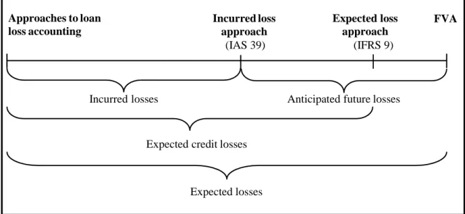
losses are recognised varies significantly across different loan loss accounting approaches, as shown in Figure 1 below. Under the assumption that LGD is constant, differences in loan loss recognition arise from the extent that changes in PDt are considered, which information (It) is used to determine PD (past versus future), and from the discount rate (dr) used to account for the time value of money.
As is evident from Figure 1, only fair value accounting (FVA) incorporates all expected losses arising both from changes in credit risk (as reflected in changes in PD) and from changes in market interest rates (dr). Therefore, FVA corresponds to the economic valuation of loans. In the following subsections, I benchmark loan loss recognition under the IAS 39 incurred loss approach and the IFRS 9 expected loss approach against economic valuation.
{Insert Figure 1 about here}
2.2. Incurred loss approach under IAS 39
Under the current incurred loss approach of IAS 39, banks may only provide for credit risk when there is ‘objective evidence’ that impairment has occurred, as of the balance sheet date (paragraph 58).3 IAS 39 paragraph 59 provides a non-exclusive list of ‘trigger events’ that are indicators of impairment. Reporting entities are not allowed to incorporate the effects of future events occurring after the balance sheet date, even if they are expected. General loan loss provisions for unspecified credit risks as allowed or required under several domestic accounting standards in Europe are not accepted under the IAS 39 rules.4
Combined with a very restrictive attitude towards loan loss provisioning, the application of the incurred loss model can result in impairments that are recognised just before default occurs (i.e., too late) (Hoogervorst, 2014). Essentially, this means that loan losses are only considered when the PD is close to 100 %. Thus, even when bank management has information (It) available about future losses, he or she is not allowed to incorporate this information for
accounting purposes. To calculate the present value of expected losses that are deemed to be incurred the original effective interest rate has to be used as the discount rate (dr). Figure 1 highlights that from the continuum of possible estimates of expected losses incurred losses represent the lowest boundary (Gebhardt and Novotny-Farkas, 2011).
2.3. The expected loss approach under IFRS 9
IFRS 9 significantly broadens the information set that an entity is required to consider when determining its expectations of credit losses.5 Specifically, reporting entities are required to incorporate information from past events, current conditions, as well as reasonable and supportable forecasts in their measurement of ECL (paragraph 5.5.17 littera c). Importantly, the new standard eliminates the threshold, i.e., the ‘trigger event’ requirement of IAS 39 for the recognition of credit losses. Reporting entities always have to account for ECLs, i.e. from the point they are first recognised, and periodically update the loan loss allowance for changes in ECLs (paragraph IN9).
2.3.1. The three stages of credit risk
IFRS 9 differentiates between three stages of credit risk. Stage 1 includes financial instruments with no significant increase in credit risk since initial recognition, or financial instruments that have low credit risk at the reporting date. The major part of banks’ performing loan portfolio will be classified as Stage 1. For these assets, 12-month ECLs are recognised in profit or loss. 12-month ECLs are expected credit losses that result from default events that are possible within 12 months after the reporting date (i.e., 12-month ECL = 12 month PD x LGD). The recognition of 12-month ECLs aims to reflect that the yield on the instrument includes a return to cover those credit losses expected from when a financial instrument is first recognised. It addresses the concern raised with respect to the IAS 39 model that it overstates interest revenue (Basis for Conclusions paragraph 5.83). Specifically, under the IAS 39 impairment model the full yield is
recognised as interest revenue with no adjustment for credit losses that are expected at the time of the origination or purchase of an asset.
Stage 2 includes financial instruments with ‘significant deterioration in credit quality’ since initial recognition, but with no objective evidence of impairment. A significant proportion of financial assets that are currently disclosed under the label ‘Financial assets past due, but not impaired’ in bank financial statements would largely fall into Stage 2 under IFRS 9. For Stage 2 assets lifetime ECLs must be recognised. This accounting treatment is based on the rationale that an economic loss arises when ECLs significantly exceed initial expectations.6 By recognising lifetime ECLs following a significant increase in credit risk this economic loss is reflected in the financial statements.
Finally, Stage 3 comprises financial instruments for which objective evidence indicates impairment at the reporting date. For Stage 3 assets, lifetime ECLs are recognised. Stage 3 credit exposures are similar to those deemed to be individually impaired under IAS 39, while Stage 1 and 2 credit exposures will essentially replace those exposures that are collectively assessed for impairment under IAS 39 (EY, 2014, p. 8). Therefore, the recognition of lifetime ECLs will occur earlier than under IAS 39, i.e., already when there is a significant increase in credit risk (Stage 2), but before actual default (Stage 3).
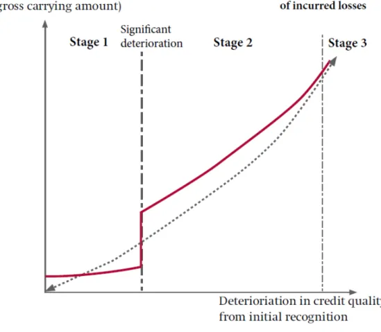
In Figure 1, the IFRS 9 expected loss model is positioned between the IAS 39 incurred loss approach and fair value accounting, because it recognises ECLs but ignores changes in market interest rates. The three-stage model of IFRS 9 tries to approximate economic ECLs that conceptually were most faithfully represented by the expected cash flow model originally proposed by the IASB in the Exposure Draft ED/2009/12 Financial Instruments: Amortised Cost and Impairment (ED 2009 model) (IASB, 2009). In the ED 2009 model, initial ECLs would be recognised over the life of an asset through the credit-adjusted effective interest rate.7 As illustrated by the curved dashed line (‘Economic expected credit losses’) in Figure 2, at
initial recognition, the loan loss allowance would be nil and subsequently built up over the life of a financial asset. This would effectively ‘match’ the recognition of credit losses with that of the credit spread implicit in the interest rates charged. Subsequent changes in ECLs would be recognised in profit or loss using the original effective interest rate(EY, 2014, p. 4). This model would come closest to the economic valuation of the loan (except that changes in market interest rates would not be recognised). However, because this model was perceived as operationally too challenging, it has not been implemented.
The solid red line in Figure 2 illustrates that the IFRS 9 three-stage model results in a stepped profile as compared to the more continuous profile of the ED 2009 model. Initially, the IFRS 9 model overstates the loan loss allowance, then - as credit risk (PD) increases - it understates the loan loss allowance, and when deterioration in credit quality is deemed significant, it again overstates the allowance.
{Insert Figure 2 about here}
2.3.2. Expected loss of financial assets (debt instruments) at fair value through other comprehensive income (FV-OCI)
An important difference relative to IAS 39 is that IFRS 9 now applies the same impairment model for financial assets through other comprehensive income (FV-OCI) as for assets recognised at amortised cost. However, unlike for assets measured at amortised cost, there is no separate allowance account for FV-OCI assets. Impairment gains and losses are recognised in the revaluation reserve in accumulated other comprehensive income and charged against profit or loss. Conceptually, this means that management estimates of 12-month or lifetime ECLs are charged to income, while other credit related changes in fair value (e.g., due to changes in market credit default swap spreads) and non-credit related changes (due to changes in interest rates and liquidity) are recognised in accumulated other comprehensive income. The new requirement will lead to an earlier recognition of credit risk associated with listed debt
instruments in profit or loss, which is particularly relevant for riskier securities that are currently held in banks’ available-for-sale portfolio which might be classified as FV-OCI under IFRS 9 (e.g., mortgage backed securities, some sovereign bonds) (see also Section 3.2.4 and Gebhardt, 2016).
3. Interaction of IFRS 9 with supervisory rules
3.1. Objectives of financial reporting and bank supervision/regulation
Since regulators use financial statement information to calculate regulatory capital numbers and rely on market participants to trade on this information to discipline banks, financial reporting and bank supervision are closely intertwined (e.g., Barth and Landsman, 2010; Bushman and Landsman, 2010). Given that the loan loss provision is the key accrual item in bank financial statements, which has a significant impact on earnings and regulatory capital, both accounting standard setters and regulators are concerned about the estimation of loan losses, but each has a different perspective on this matter.8
The differences in accounting versus supervisory perspectives on loan loss provisioning result from the fact that financial reporting and bank supervision pursue different objectives. Supervisors’ primary objective is to reduce the level of risk to which depositors are exposed and to maintain financial stability. Regulators have different informational needs than, for example, investors, because they face an asymmetric loss function. Specifically, understated loan loss allowances (overstated regulatory capital) may increase the probability of a bank failure and increase the cost imposed on deposit insurance systems, and ultimately tax payers. In contrast, overstated loan loss allowances do not impose costs to supervisors (Benston and Wall, 2005). Therefore, from the range of estimates for potential loan losses, supervisors prefer that loan losses are valued at the higher end of these estimates. In contrast, the main objective of financial
reporting is to provide information that is useful to a wide range of financial statement users, including investors, creditors and regulators.
Bank supervisors have different tools at their disposal to discipline banks’ risk taking, and in turn, to enhance financial stability. Specifically, since the introduction of Basel II, bank regulation has been resting on three pillars. Pillar 1 requires banks to hold a minimum amount of regulatory capital that reflects the riskiness of banks’ assets. Minimum capital requirements reduce risk taking incentives by inducing bank owners to raise capital and place more of their personal wealth at risk in the bank, when they invest in more risky assets (Kim and Santomero, 1988). Pillar 2 – supervisory review – provides supervisors with the authority to evaluate banks’ risk management practices and to impose more stringent capital requirements if they deem a bank’s capitalisation to be inadequate. Pillar 3 – market discipline – requires transparent reporting that enables capital markets to serve as a complementary force to discipline banks’ behaviour. Financial reporting, and in particular loan loss provisioning, and bank supervision intersect at all three pillars as I discuss in more detail in the following sections.9
3.2. IFRS 9 and bank capital (Pillar 1)
Bank regulators use accounting numbers as inputs to regulatory capital calculations. However, to preserve the prudential role of regulatory capital, they make certain adjustments to reported financial statement numbers. In the following subsections, I elaborate on differences in the measurement of expected losses in IFRS 9 versus Basel III and discuss how these differences are reflected in regulatory capital calculations. In doing so, I refer to the provisions of Basel III as they are implemented in the EU in the Capital Requirements Regulation (CRR)10 and the Capital Regulation Directive IV (CRD IV)11, where appropriate.
3.2.1. Definition of default
As the definition of default sets the basis for the estimation for the key inputs into expected loss calculations, a consistent and comparable definition is essential (EBA, 2015a). For example, a 9
too narrow definition of default would increase the identified number of defaults, i.e., would result in higher probability of default (PD). In contrast, the loss given default (LGD) would decrease, because a larger number of defaults would be considered, where the actual loss would be small or even zero (Grünberger, 2013). Therefore, it is crucial that default is clearly defined and consistently applied through time.
The definition of default in the capital adequacy framework focuses on two main indicators. First, the qualitative indicator refers to obligor’s unlikeliness to pay its credit obligations.12 Article 178 paragraph 3 of the CRR lists the main elements to be taken as indications of ‘unlikeliness to pay’. Second, the quantitative indicator refers to the credit obligations with past due status for more than 90 days.13
The IASB decided not to define default in IFRS 9 because it might result in a definition for financial reporting that is inconsistent with that applied internally for credit risk management (Basis for Conclusions paragraph 5.251). Instead, entities should apply a definition of default that is consistent with the definition of default for internal credit risk management purposes, consistently from one period to another. However, IFRS 9 introduces a rebuttable presumption that default occurs when a financial asset is more than 90 days past due (paragraph B5.5.37). This presumption serves as a ‘backstop’ to ensure that entities do not define default later than 90 days without reasonable and supportable information. In addition, Appendix A to IFRS 9 provides a list of indicators providing evidence that a financial asset is credit-impaired that entities should consider.
Both, the quantitative and qualitative indicators of default, are essentially similar in the accounting and regulatory framework. However, in practice there are large discrepancies in the definition of default across Member States that partly stem from different supervisory practices and national regulations in various EU jurisdictions (EBA, 2015a).
3.2.2. Expected loss under IFRS 9 versus expected loss under CRR
Generally, the IFRS 9 expected loss approach brings loan loss provisioning closer to the regulatory methodology of measuring expected losses. Specifically, the Stage 1 12-month expected loss is conceptually similar to the regulatory expected loss that has also a 12-month horizon. Under both frameworks, the key input parameters for the measurement of expected loss are the probability of default (PD) and the loss given default (LGD). Therefore, it is not surprising that the IASB ‘expects entities to be able to use some regulatory measures as a basis for the calculation of expected credit losses in accordance with the requirements in IFRS 9’ (Basis for Conclusions paragraph 5.283).
However, because of the different objectives of regulation and financial reporting, the regulatory estimates of PD and LGD are not the same as those that shall be used for expected loss calculation of expected losses under IFRS 9. Hence, these estimates have to be adjusted to meet the measurement requirements of IFRS 9 (Basis for Conclusions paragraph 5.283).
IFRS 9 expected loss and regulatory expected loss requirements differ in their scope of application. The regulatory measurement and treatment of loan loss provisions depend on whether banks use the Standardised Approach (SA) or the Internal Ratings-Based (IRB) Approach for calculating their capital requirements for credit risk. Under the SA approach banks are required to use external credit ratings to quantify the required amount of capital for credit risk. For unrated exposures SA banks have to apply predetermined risk weights as defined in the regulatory capital framework (see CRR Section 2). In contrast, under the IRB approach, which is subject to regulatory approval, banks can use their own estimated credit risk parameters to calculate the required amount of capital. Regulatory expected loss rules are relevant only for IRB banks. In contrast, the scope of expected loss provisions of IFRS 9 includes all assets measured at amortised cost and FV-OCI, and therefore, is also relevant for SA banks.
For SA banks, regulation generally does not prescribe the measurement of regulatory loan loss provisions. Instead, accounting provisions directly affect Tier 1 capital. However, some countries require specific regulatory provisioning rules based on a combination of supervisory loan classification (e.g. Pass, Special Mention, Substandard, Doubtful) and corresponding loan loss rates that have to be applied to each category (World Bank, 2002; Gaston and Song, 2014).
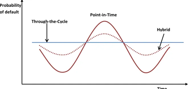
In contrast, IRB banks must calculate the expected loss using their own estimates of PD and LGD for non-defaulted (i.e., performing) exposures. The rating philosophy for PD estimates may follow a point-in-time (PiT), through-the-cycle (TTC) or a hybrid approach. PiT ratings represent an assessment of the borrower’s probability of default over a relatively short horizon (e.g., a year), and thus, can vary considerably over the business cycle. The TTC approach focuses on a longer horizon, essentially neutralising the effects of current cyclical conditions, and therefore results in more stable and less cyclical ratings. In contrast, PiT PDs vary more significantly from expansionary to recessionary periods. The hybrid approach is a combination of TTC and PiT models, which means that PD ratings are calibrated to long run default rates but adjusted to reflect current economic conditions. Figure 3 illustrates how PD estimates vary over the business cycle depending on the underlying rating philosophy.
{Insert Figure 3 about here}
The CRR does not require a specific rating philosophy but clarifies that PD estimates should reflect the long run average of one-year default rates in order to ensure that they are relatively stable over time.14 This would suggest that only through-the-cycle approaches (i.e., TTC or hybrid) are consistent with the capital adequacy framework.15 For defaulted exposures banks must use their best estimate of expected losses given current economic conditions and exposure status taking into account the estimate of the increase of loss rate caused by possible additional losses during the recovery period.16
The IASB clarifies that TTC estimates are not consistent with IFRS 9 expected loss requirements because they ‘consider a range of possible economic outcomes instead of those that are actually expected at the reporting date. This would result in a loss allowance that does not reflect the economic characteristics of the financial instruments at the reporting date’ (Basis for Conclusions paragraph 5.282).17 Specifically, as shown in Figure 3, TTC estimates are likely to overstate PiT PDs during boom periods and understate PiT PDs during downturns. Therefore, regulatory PDs will need to be adjusted to reflect current and forecast economic conditions.
Further differences arise with regard to the estimation of the LGD. The CRR requires the estimation of LGD based on the long run average weighted by the number of defaults. However, downturn LGDs should be used, if those are more conservative than the long run average. Downturn LGD refers to the LGD in an economic downturn. Under IFRS 9 LGDs should incorporate actual expectations of the future at a given reporting date.18 In addition, under the capital adequacy framework, the less information a bank has the more conservative should its PD and LGD estimates be.19 In addition, the regulatory parameters have floors. These conservative biases are inconsistent with the IFRS 9 expected loss approach and need to be removed.20
Finally, the regulatory expected loss is always calculated over a 12-month horizon for performing portfolios, while under IFRS 9 lifetime losses have to be recognised for the part of the performing portfolio, for which credit risk has significantly increased (i.e., Stage 2 assets). For defaulted assets lifetime losses have to be recognised under both frameworks.
3.2.3. Loan loss provisions and regulatory capital
The measurement of loan loss provisions is directly linked to capital ratio calculations. Like the measurement of expected losses, the regulatory treatment of loan loss provisions also depends on whether a bank uses the SA or the IRB approach to measure credit risk.
Under the SA, banks are allowed to include general loan loss provisions in Tier 2 capital subject to the limit of 1.25 % of risk-weighted assets (Article 62c CRR). ‘Collective impairment provisions’ under IFRS 9 will only be eligible for inclusion in Tier 2 capital, if (1) they are freely and fully available, as regards to timing and amount, to meet credit risk losses that have not yet materialised, and (2) they reflect credit risk losses for a group of exposures for which the institution has currently no evidence that a loss event has occurred.21 As noted before, some jurisdictions apply supervisory loan loss provisioning rules to ensure a minimum level of provisions. In these jurisdictions, if the supervisory provisions are in excess of accounting loan loss provisions, the difference is deducted from Tier 1 capital.
The capital treatment under the IRB approach is based on the rationale that loan loss provisions should cover expected losses, while unexpected loan losses should be absorbed by regulatory capital. Consistent with this concept, any shortfall arising from the comparison of supervisory and accounting expected loss has to be deducted from Tier 1 capital (i.e., when the supervisory expected loss is greater than the expected loss recognised in accounting through loan loss provisions) (Article 36d CRR). In this respect, the new Basel III regulatory framework is more stringent than Basel II, where 50 % of the IRB shortfall was deducted from Tier 1 and 50 % from Tier 2. The excess of eligible accounting loan loss provisions over supervisory expected losses can be included in Tier 2 capital up to 0.6 % of risk weighted assets (RWA) (Article 62d CRR). Figure 4 illustrates the regulatory capital treatment of differences between regulatory and IFRS 9 expected losses for IRB banks.
{Insert Figure 4 about here}
Based on the discussion above it is expected that IFRS 9 impairments will particularly have an impact on regulatory capital for SA banks. The regulatory capital impact for IRB portfolios will be more moderate and will depend on the level of new impairment provisions relative to the regulatory expected loss. Because regulatory expected loss is based on TTC estimates, while
IFRS 9 requires PiT estimates, accounting impairment provisions will be generally below regulatory expected loss during benign economic conditions. In a downturn, IFRS 9 impairments might be larger than regulatory expected loss, because of the PiT PDs which will be larger than TTC PDs and banks will have to increasingly recognise lifetime losses in Stage 2 and Stage 3. While these ‘excess provisions’ will reduce Tier 1 capital, they can be included as part of Tier 2 capital up to a limit of 0.6 % of risk-weighted assets (RWA). An illustration of how TTC estimates versus PiT estimates of loan losses behave over the business cycle is provided in the Pillar 3 report of Barclays included in Appendix A. In contrast to IRB banks, SA banks will experience a one-to-one impact of increased loan loss allowances on their Tier 1 capital.
3.2.4. Prudential filters in CRR and expected losses under IFRS 9 on FV-OCI debt securities
Under previous capital adequacy requirements, unrealised fair value gains or losses recognised on debt instruments held in the available-for-sale (AFS) portfolio as other comprehensive income were neutralised in the calculation of regulatory capital through the application of prudential filters. The rationale behind this prudential treatment was to avoid the excessive volatility of regulatory capital stemming from (presumably temporary) changes in the fair value of banks’ securities portfolio (e.g., Laux, 2012). Indeed, during the financial crisis the application of prudential filters acted as a safeguard by shielding banks from unrealised fair value losses (Laux and Leuz, 2010). However, because these debt securities are essentially recognised at amortised cost for prudential purposes, the regulatory capital constraint has less bite. Specifically, deteriorations in the value of these assets do not affect regulatory capital until impairment is recognised, which under incurred loss approach can be delayed until late. This favourable prudential and accounting treatment provided ex ante incentives for risk shifting (Lu et al., 2012; Chircop and Novotny-Farkas, 2016).22
Regulators have recognised this issue and under the new capital adequacy framework they require unrealised gains and losses on AFS assets to be included in the calculation of regulatory capital (Article 35 CRR). This regulatory change further aligns accounting and bank regulation. The CRR includes transitional provisions for the stepwise removal of the prudential filters applied to AFS debt securities under IAS 39.23 Remarkably, these transitional provisions allow institutions ‘not to include in any element of own funds unrealised gains or losses on exposures to central governments classified in the ‘‘Available for Sale’’ category of EU-endorsed IAS 39’ (Article 467 paragraph 2 CRR) if permitted by the supervisor. Indeed, many EU supervisors chose to use this option particularly in those Member States whose banks built up substantial (domestic) sovereign risk in their portfolios in recent years (e.g., Belgium, Cyprus, Ireland, Italy, Portugal and Spain).24
This supervisory option is a cause of concern, because it allows banks to invest in risky sovereign exposures without recognising unrealised gains and losses in regulatory capital. The issue is further exacerbated by the fact that under CRR, banks can essentially apply a zero risk weight to sovereign exposures. Specifically, under the SA, exposures to central banks and to Member States’ sovereign debt issued in the domestic currency are assigned a zero risk weight. In the euro area, this automatically applies to all banks, resulting in a favourable treatment of sovereign bonds despite significant actual differences in credit risk (ESRB, 2015). In addition, while in theory IRB approach banks would have to assign risk weights according to their internal ratings, the CRR allows these banks to apply the SA to sovereign exposures (‘permanent partial use’).25 This option has been used by many IRB banks.26 Moreover, increases in the credit risk of sovereign debt securities do not result in capital charges either, because the current IAS 39 accounting rules allow delaying impairment until too late (Gebhardt, 2016).
The combination of the preferential regulatory and accounting treatment of sovereign debt essentially provides a ‘sovereign subsidy’ to EU banks, the value of which increases with the riskiness of the underlying sovereign exposure (Korte and Steffen, 2015).27 In fact, the current regulatory and accounting framework might explain why particularly banks located in GIIPS countries (i.e., Greece, Italy, Ireland, Portugal, Spain) increased primarily their domestic sovereign exposures since the beginning of the sovereign debt crisis (Acharya and Steffen, 2015). As a consequence of these incentives, bank and sovereign default risk become more closely intertwined, which poses a further threat to financial stability in the EU.
The above mentioned concerns might be mitigated to some extent by the adoption of IFRS 9 (if consistently applied). Under IFRS 9, the AFS category will not exist, and financial assets classified in the FV-OCI category under IFRS 9 will not be subject to prudential filters under the CRR (EBA, 2015b). Therefore, if sovereign exposures will be classified as FV-OCI, fair value gains and losses will affect regulatory capital. Banks might classify riskier exposures in the amortised cost category and still benefit from the zero risk weight under CRR. However, because the expected loss approach of IFRS 9 will apply to all assets of the banking book, the riskiness of the sovereign debt securities will be reflected in both - income and regulatory capital - through the recognition of Stage 1 12-month expected losses at each reporting date. Further, significant increases in sovereign credit risk will be recognised and charged to regulatory capital earlier through lifetime impairments in Stage 2.28 The larger and earlier regulatory capital charges might reduce banks’ incentives to excessively invest in risky sovereign bonds, which in turn, would enhance financial stability.
3.3. IFRS 9 and the supervisory review process (Pillar 2) 3.3.1. Supervisory evaluation of loan loss provisioning
The supervisory review process (Pillar 2 of the Basel framework)29 is relevant for loan loss provisioning on primarily two levels, which are emphasised in the Basel Committee’s Core Principles for Effective Banking Supervision (BCBS, 2012). First, supervisors are responsible for assessing whether banks have appropriate credit risk management practices in place.30 Given that the IFRS 9 expected loss approach specifically relies on data generated by banks’ internal credit risk models, the supervisory evaluation and validation of these models will become even more important in ensuring a high-quality and consistent application of IFRS 9 requirements. Second, they need to evaluate whether adequate policies are in place for the early identification of problem assets and whether reported loan loss allowances are adequate.31 If the supervisors detect material deficiencies in banks’ risk management processes or in the level of loan loss allowances they have the power to impose capital add-ons (‘Pillar 2 add-ons’).32
The above mentioned roles of supervisors are further reinforced by the Basel Committee’s recently issued (draft) Guidelines on accounting for expected credit losses (BCBS, 2015a). The Guidelines also stress the role of supervisors in ensuring that the methods used by banks to determine loan loss allowances produce a robust measurement of expected losses under the applicable accounting framework. Although compliance with accounting standards lies primarily in the responsibility of management, auditors and enforcement bodies, the BCBS Guidelines implicitly suggest that supervisors should support enforcement of consistent implementation of IFRS.33 In doing so, they may cooperate with internal and external auditors in reviewing a bank’s credit risk assessment and ECL measurement functions (BCBS, 2015a, paragraph 85).
3.3.2. Consistency in supervisory practices The Basel Committee
‘emphasizes the importance of a high quality, robust and consistent implementation of ECL accounting frameworks across all jurisdictions’ and it aims ‘to drive consistent interpretation and practices, where there are commonalities and when the same accounting framework is applied’ (BCBS, 2015a, paragraph 3).
This emphasis on consistency in the current guidance stems from the experience with the IAS 39 incurred loss model that has been implemented with significant differences across and even within jurisdictions because of different national, regional and entity specific practices and interpretations.34 In addition, differences in loan loss provisioning practice also arise, because supervisors vary in their willingness, ability and power to act and to intervene in loan loss provisioning (e.g., Gaston and Song, 2014). The potential for diverging interpretation of loan loss accounting rules is even greater under the expected losses approach of IFRS 9, since it widens the scope for judgement. Therefore, while the Basel Committee’s Guidelines represent an important step towards a common supervisory understanding, consistency in the implementation and application of the IFRS 9 requirements will largely depend on the harmonisation of supervisory practices within the European Union. In this regard, the recent efforts of the EBA are crucial in achieving supervisory consistency and convergence of supervisory practices in the European Union.35
It should be noted, that consistent supervisory practices can only achieve consistency in inputs used in the recognition and measurement of ECLs, but not consistent outputs because of inherently different business and risk management models across banks. Relatedly, supervisors should not strive to intervene into loan loss provisioning in order to obtain a specific outcome that meets supervisory goals, which would compromise the objective of financial reporting to provide useful information to a broad range of financial statement users.
While the Basel Committee’s Guidelines acknowledge the different objectives of financial reporting and bank supervision, it sets out certain supervisory expectations with respect to the 19
measurement of 12-month ECL and the determination of ‘significant increases’ in credit risk. In addition, it limits the use of practical expedients provided in IFRS 9. The Guidance in these areas reflects the Basel Committee’s preference for more conservative loan loss provisioning. For example, the Guidelines emphasise that nil 12-month ECL allowances should be rare and that the methodology used to estimate 12-month ECL should allow for the more timely build-up of allowances. Further, the BCBS expects that the definition of default is guided by the definition used for regulatory purposes (see Section 3.2.1), emphasising that the regulatory qualitative criterion ‘unlikeliness to pay’ should be the primary indicator while the 90-day-past due status should only serve as a ‘backstop’.36
The Guidelines will be used not only by national supervisory authorities, but also by auditors (KPMG, 2015). Depending on the interpretation by these parties, it bears the risk of being implemented too restrictively and thereby not only imposing significant costs on banks, but also biasing the measurement of ECL towards a more conservative estimation. Furthermore, the interpretation of the Guidelines might vary across jurisdictions.
An example of how a specific supervisory interpretation of loan loss accounting rules might endanger the integrity of financial reporting is provided by the Spanish case. In Spain the Banco de España has the authority to set accounting standards for banks and it introduced a so called ‘dynamic provisioning’ approach in the year 2000. Under this approach, in addition to the ‘normal’ loan loss provisions, banks had to set aside statistical provisions based on either their own internal ratings or predetermined loss rates assigned to different classes of risk exposures. The rationale behind this statistical provision is to build up a reserve during good times, when loan growth is high, that can be depleted during bad times. Upon transition to IFRS, these reserves should have been reversed, because they were inconsistent with the IAS 39 incurred loss approach. However, the Banco de España actually forced its banks to continue the dynamic provisioning regime under IFRS. At transition, instead of reversing statistical reserves that had
been separately disclosed under Spanish accounting rules, Spanish banks actually merged them with general loan loss provisions, and labelled the resulting amount as ‘collective impairments’ under IFRS. Not only was this procedure incompatible with IAS 39 requirements, but it also made loan loss provisioning in Spain less transparent (Novotny-Farkas, 2011). In addition, the reserves built up during good times could be used by banks to hide losses until these reserves were depleted. This allowed banks to look healthy (sometimes for several years), when they were actually in financial distress. Ultimately, several Spanish banks crashed and had to be bailed out after their reserves had been depleted and hidden losses materialised (Bloomberg, 2012).
3.4. IFRS 9 and market discipline (Pillar 3)
3.4.1. Loan loss provisioning and market discipline
A large theoretical literature in banking posits that informational transparency of banks plays a fundamental role in promoting market discipline as a complementary force in bank supervision.37 The increased emphasis on market discipline as a prudential tool is exemplified by its codification in Pillar 3 of the Basel II/III capital adequacy framework and in Part 8 of the CRR. While there is no uniform definition, market discipline can be conceptualised as a mechanism by which market participants monitor and discipline excessive risk-taking of banks (e.g., Stephanou, 2010). Market discipline can operate through different channels. First, it can operate through the direct influence that market participants exert on a bank’s risk taking behaviour, for example, by penalising banks for greater risk-taking by demanding higher returns on their investment.38 Anticipating investors’ behaviour bank managers will have reduced ex ante risk taking incentives. Second, indirect market discipline can also operate through supervisory intervention triggered by market signals (e.g., price movements of bank securities)
(Stephanou, 2010). Third, market discipline can also limit the scope of regulatory forbearance by incentivising bank supervisors to promptly intervene in troubled banks (Rochet, 2005).
One of the main building blocks of market discipline is the public availability of adequate, timely, consistent and reliable information on the bank’s financial performance and risk exposures (Stephanou, 2010). In other words, the extent to which bank supervisors can rely on market discipline as a complementary tool in bank supervision depends on the quality of information available to capital market participants. For banks, loan loss provisioning is a key accounting item that has a significant impact on banks’ earnings and regulatory capital, and it directly influences the information properties of financial reports with respect to reflecting loan portfolios’ risk attributes (Bushman and Williams, 2012).
3.4.2. IFRS 9 and expected loss related disclosures
Since the ECL approach under IFRS 9 significantly widens the scope for managerial judgement, the extended disclosure requirements (implemented in IFRS 7, which will be applicable when IFRS 9 will apply, presumably from 1 January 2018) will play a crucial role in supporting market participants and bank supervisors in their assessment of the adequacy of ECL measurement. The newly required disclosures particularly address the aspects of the ECL approach that involve most managerial discretion including how the entity has determined ‘significant increases’ in credit risk, the definition of default, the basis of inputs and assumptions and the estimation techniques used to measure 12-month expected losses etc.39
In addition to expected loss related disclosures, banks’ Pillar 3 reports provide another set of relevant disclosures that are useful to investors and bank supervisors to evaluate credit risk inherent in banks’ portfolios. For example, for IRB banks Pillar 3 requires disclosures of the main expected loss parameters such as exposure at default (EAD), exposure-weighted PDs and LGDs for each exposure class and each relevant geographical location (Article 452 CRR). Furthermore, banks must disclose estimated losses against actual losses in each exposure class
for a sufficient period to help assess the performance of banks’ internal rating system. Where appropriate, disclosures should also include a comparison of estimated and actual PDs and LGDs (Article 452(i) CRR). An example of detailed Pillar 3 disclosures of risk parameters is provided by HSBC in 2014 in Appendix B. Such disclosures are essential for evaluating the validity and adequacy of banks’ ECL estimates. For example, Bartlett (2012) shows, using two case studies, how market participants might use the disclosure of the standard parameter estimates (such as PDs and LGDs) and even basic, textbook credit risk models to estimate banks’ exposure to credit risk and their capital position.
However, while some banks already provide information in their Pillar 3 reports that would allow a similar analysis, the extent of disclosure and compliance with Pillar 3 varies across banks in the EU as reflected in the EBA’s periodic assessment of Pillar 3 disclosures EBA (2013a). In this regard, the efforts of the EBA in this area will be crucial in order to improve the adequacy, relevance and comparability of disclosures and in identifying best practices.40 In addition to banks' specific disclosures, market participants can also use aggregate disclosures such as those provided during the EBA’s stress tests. For example, the 2011 EBA stress test disclosed the distribution of PDs and LGDs for the main credit risk exposure classes for the 90 participating EU banks (see Appendix C). Such aggregate disclosures can be used as yardsticks against which bank specific parameter estimates can be benchmarked.
4. Implications of the IFRS 9 impairment model for financial stability
4.1. The relation between loan loss accounting and financial stability
In and of itself, the underlying loan loss provisioning approach is unlikely to play a major role from a financial stability perspective. Specifically, how a bank recognises expected credit losses does not change the cash flows it receives from loans, which are determined by borrower payments (Benston and Wall, 2005). Loan loss provisioning will have an effect on financial
stability only to the extent it has an influence on banks’ real decisions in terms of investment, funding, and dividend policies. For example, earlier and higher reported loan losses will reduce a bank’s reported earnings and equity capital, which in turn, may induce a bank to undertake some combination of issuing new equity capital, reducing its dividends, and reducing its risky investments, conservative actions that it otherwise might not undertake. It is these actions that reduce the risk of bank failure and not the change in reported loan losses (Benston and Wall, 2005).
Relatedly, it is important to bear in mind that financial reporting ‘is just one piece of the larger regulatory configuration’ (Bushman and Landsman, 2010, p. 260). Financial reporting in general and loan loss provisioning in particular will only have an impact on financial stability through its interactions with other pieces of the regulatory configuration, specifically with the three Pillars of bank supervision and regulation. In this regard, it should be also noted that even market discipline does not work in a vacuum. As emphasised by Stephanou (2010), market discipline has less to do with the market per se but is more about the institutional framework that provides relevant information, the right incentives, and control used to reduce the problems of moral hazard and asymmetric information that are endemic in banking (Stephanou, 2010). For example, a more timely and transparent loan loss provisioning system is unlikely to improve market discipline, if market participants do not have proper incentives to exert discipline on banks.41
4.2. Will provisioning under IFRS 9 be less procyclical than under IAS 39?
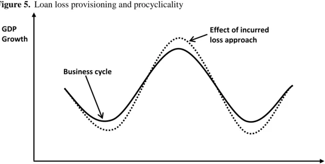
Every loan loss accounting model that aims to reflect economic conditions is naturally procyclical. From a financial stability perspective the concern is whether loan loss accounting amplifies the upward and downward swings of the business cycle as illustrated in Figure 5. This has been potentially the case under the incurred loss approach of IAS 39. During boom periods, banks can recognise risk premia included in the interest rates charged on loans but not the
matching expenses for expected credit risk. Under benign economic conditions, the probability of specific loss events that would trigger impairment under IAS 39 is low. This leads to overstated earnings and regulatory capital, which in turn, allows banks greater loan growth within the regulatory capital standards and dividend payments. In a downturn, however, previously accumulated unrealised loan losses materialise and hit regulatory capital, which compromises its ability of regulatory to cover unexpected losses. The drop in regulatory capital and the increased riskiness of loans will induce banks to either raise new equity capital or to cut lending, in order to meet the minimum regulatory capital requirements. However, as financing frictions might limit banks’ ability to raise new capital, banks might be forced to reduce their lending, which can result in a credit crunch (e.g., Gebhardt and Novotny-Farkas, 2011). In addition, market disciplining mechanisms are hampered, because markets are informed about losses only with a delay, which can further exacerbate financing frictions in a downturn (Bushman and Williams, 2015).
{Insert Figure 5 about here}
The expected loss approach under IFRS 9 can mitigate the above mentioned concerns: First, the recognition of 12-month ECL in Stage 1 in a sense serves as an adjustment to the credit spread that is recognised through the yield, and thus, results in less overstated profits. This will reduce the possibility of distributing overstated profits in the form of dividends and bonuses during boom periods and will result in more capital to withstand losses during a downturn.42 In addition, the earlier recognition of losses in regulatory capital could mitigate excessive loan growth during boom times. In fact, as noted in Section 2 and illustrated in Figure 2, the Stage 1 ECL will overstate the loan loss allowances in the beginning of the life of a loan, and thus, has a ‘buffer effect’ on regulatory capital that increases with the riskiness of newly extended loans. However, this buffer effect on regulatory capital will primarily be relevant for SA banks. For IRB banks, the regulatory expected loss buffer is likely to exceed the IFRS 12-month ECLs
during upswings, because the former is based on through-the-cycle PDs and downturn LGDs, while the latter is calculated using point-in-time estimates. In contrast, during economic downturns accounting expected losses will exceed the regulatory expected losses not only because PiT estimates will be larger than TTC estimates, but because accounting impairments will increasingly recognise lifetime losses in Stage 2 and Stage 3 (see Sections 3.2.2 and 3.2.3). Second, the more timely recognition of loan losses and extended disclosures will promote market discipline. In particular, providing earlier information about (increases in) credit risk to market participants may reduce financing frictions in times of financial stress.
Taken together, the IFRS 9 expected loss model is likely to mitigate the effect of the features of IAS 39 that potentially amplified procyclicality. That being said, I believe that the expected loss approach will by construction reflect natural procyclicality in the economy. Specifically, because the parameter inputs used in estimating ECLs are PiT estimates they will oscillate with the business cycle (see Figure 3). This means that ECLs will be lower during upswings and significantly larger during downswings. Indirect evidence on this is provided by empirical studies that examine the procyclicality of regulatory capital. This literature suggests that IRB banks that compute PIT PDs produce highly significant variations in regulatory capital from expansionary to recessionary periods, as opposed to IRB banks that compute TTC PDs.43
The extent to which the ECL model will be procyclical will largely depend on how it is implemented. For example, in a simulation study Grünberger (2014) shows that the 2013 ED model is procyclical, but this procyclicality is mitigated if forward PDs are considered. However, the estimation of forward looking PDs is challenging and many banks will not have yet the systems and the relevant information to estimate them reliably (Grünberger, 2014).44 Relatedly, if banks are not able to identify ‘significant increases’ in credit risk on a timely basis, significant ‘cliff effects’ are possible, when banks’ loans switch from Stage 1 to Stage 2, i.e.,
when they transition to lifetime losses recognition.45 This can significantly increase the volatility of regulatory capital.46
4.3. Discretionary loan loss provisioning
The IFRS 9 expected loss model introduces a significant amount of managerial discretion over the timing and measurement of expected losses. With regard to timing, there is substantial scope for judgment in determining significant increases in credit risk that trigger the switch from 12-month ECL to the recognition of lifetime losses. To avoid the above mentioned ‘cliff effects’ management might be inclined to delay the movement of assets from Stage 1 to Stage 2. In this case, recognised impairments would also be ‘too little too late’. In a downturn, when problems unfold quickly, the initial delay of the recognition of Stage 2 losses can exacerbate the ‘cliff effect’ with a sudden and substantial increase in loan loss allowances and a hit to regulatory capital creating the same problems as observed with IAS 39’s incurred loss model. In addition, the longer the forecast horizon that has to be considered in the measurement of expected losses the greater the valuation uncertainty and subjectivity.
As widely acknowledged in the accounting literature, discretion is a double edged sword (e.g., Bushman and Landsman, 2010; Bushman, 2016). On the one hand, discretion allows bank managers to incorporate private information about future credit losses. On the other hand, discretion might be used opportunistically to prop up reported earnings and regulatory capital. Managerial incentives for opportunistic accounting choices are primarily provided by executive compensation, capital market pressures and capital inadequacy concerns. The closer alignment between accounting and the new bank regulation under CRR will further reinforce these incentives. The combination of higher minimum regulatory capital requirements under CRR and larger loan loss allowances will increase the likelihood that certain regulatory thresholds, e.g., the capital conservation buffer, are breached, which automatically will limit dividends and bonus payments. Therefore, management will probably have even stronger incentives and
greater opportunity under the expected loss approach to delay the recognition of losses and to smooth income.
The recent literature examining discretionary loan loss accounting choices highlights that managerial discretion can detrimentally affect financial stability through two distinct accounting channels (see Section 5.2): First, it can exacerbate capital inadequacy concerns during economic downturns by compromising the ability of loan loss allowances to cover both unexpected recessionary loan losses and loss overhangs from previously unrecognised losses. Second, discretionary loan loss provisions degrade transparency which can exacerbate financing frictions and hamper market discipline of bank risk taking. Capital inadequacy concerns in combination with high financing frictions can increase bank fragility, while capital inadequacy combined with weak market discipline can provide strong incentives for banks to engage in risk-shifting behaviour (Bushman, 2016).
Therefore, particularly in the context of expected loss accounting extensive disclosure of information related to the inputs, assumptions and techniques used to identify significant increases in credit risk and to estimate ECLs will be crucial. Unfortunately, the disclosure requirements do not include a comparison of previous estimates of ECLs with actual outcomes (‘back-testing’). This information would help users of financial statements to assess the ability of management to predict future losses and the extent to which prior loan loss provisions were over- or understated which in turn could mitigate discretionary behaviour. Such disclosure was proposed in the Supplementary Document (SD) in 2011 (IASB, 2011, paragraph Z12), but the IASB removed this provision following opposition from respondents to the SD. Respondents argued that ‘back-testing on expected credit loss amounts would not provide useful information, and could be misleading because estimates of expected credit losses necessarily require judgement’ (IASB, 2013b, Basis for Conclusions paragraph 109). However, precisely because of the judgemental nature of ECL estimates, back-testing disclosures would be necessary and
useful. Moreover, banks also provide such disclosures for regulatory expected loss estimates in their Pillar 3 reports.
5. Insights from the empirical accounting literature
In the accounting literature there is ample empirical evidence that loan loss provisions have been used for earnings, tax and capital management.47 In this section, I will focus on the discussion of studies that provide some insights on the specific issues discussed in Chapters 3 and 4. First, I describe the impact of the adoption of IAS 39’s incurred loss approach on loan loss provisions of European banks. Then, I discuss selected recent studies that examine the economic consequences of discretionary loan loss provisioning, particularly in the context of financial stability.48
5.1. The impact of IAS 39 on loan loss provisioning in Europe and the interaction with bank supervision
Before the mandatory introduction of IFRS in the EU in 2005, local GAAP rules for loan loss provisioning were based on the EC Bank Accounts Directive49, which allowed banks, at least in part, to anticipate the losses expected to occur due to future events. The largely principles-based rules left considerable leeway in how they were applied, which resulted in different loan loss provisioning practices across EU Member States. This diversity stemmed partly from different tax and regulatory treatment of loan loss allowances, and, in particular, from the extent of supervisory intervention into loan loss provisioning. For example, as mentioned above, the Spanish supervisor, the Banco de España introduced a dynamic loan loss provisioning regime. The Danish Financial Services Authority required banks to recognise all potential future losses in their loan loss provisions in order to approximate the market value of loans(Bernard et al., 1995; Gebhardt and Novotny-Farkas, 2011). However, in practice, this probably just meant a
very conservative way of loan loss provisioning as reflected in the following statement of Denmark's Nationalbank:
Under the previous accounting rules based on the prudential principle the banking institutions’ loan loss provisions were not necessarily reflected in losses whereby the accumulated provisions partly served as buffer(Danmarks Nationalbank, 2006, p. 27). Loan loss accounting under IAS 39 differs from local GAAPs with regard to two main features. First, under IAS 39 banks can recognise only incurred losses; the recognition of losses expected as a result of future events is not permitted. Second, to determine the impairment loss, the expected future cash flows have to be discounted using the original effective interest rate.
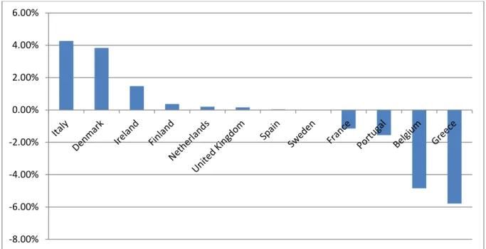
In contrast, local GAAP rules allowed or even required to consider future losses and the prevailing practice was to use the sum of undiscounted future cash flows to measure the amount of impairment loss (Gebhardt and Novotny-Farkas, 2011). This means that upon transition to IFRS/IAS 39, one would expect to see two countervailing effects on the level of loan loss allowances. On the one hand, we should observe a decrease in loan loss allowances due to the reversal of provisions that go beyond incurred losses. On the other hand, the measurement of impairment losses based on discounted cash flows should result in an increase in loan loss allowances (Novotny-Farkas, 2011, pp. 30-31). Figure 6 presents the median net impact of changes in loan loss allowances upon transition to IFRS on shareholders’ equity for 87 banks from twelve EU countries.
{Insert Figure 6 about here}
In terms of the transitional impact of changes in loan loss allowances three major country clusters can be identified in Figure 6. There is a group of countries that experienced a significant decrease (increase) in loan loss allowances (in shareholders’ equity) reflecting previous ‘over-reserving’ (e.g., Italy and Denmark). Another group of countries show only a minimal change in their median level of loan loss allowances (e.g., Finland, Netherlands, United Kingdom, Sweden). These countries had local GAAP provisioning rules that were similar to those in IAS
39. Finally, there is a cluster of countries that experienced a significant increase (decrease) in loan loss allowances (shareholders’ equity) which is primarily attributable to the effect of discounting.
Interestingly, the median impact of IAS 39 on loan loss allowances is zero for Spanish banks. One would have expected to observe significant reversals of statistical provisions built up under the dynamic provisioning regime, which are inconsistent with IAS 39’s incurred loss approach. However, as discussed in Section 3.3.2., the Spanish supervisor required its banks to maintain the dynamic provisioning model even under IFRS. The transition effects of Spanish banks provide empirical evidence of the Spanish supervisors’ resistance to comply with IAS 39. In contrast, as expected, Danish banks reversed significant portions of their excess reserves built up due to the application of the Danish ‘mark-to-market’ accounting rules. Thus, unlike in Spain, the Danish supervisor accepted the primacy of IFRS as the accounting framework for Danish banks. Consistent with this argument, Danmarks Nationalbank notes that the ‘new accounting rules’ for banks (i.e., IFRS) ‘entail that provisions for future losses must no longer be based on a prudential principle, but on a neutrality principle’ (Danmarks Nationalbank, 2007, p. 71).
The rationale behind the restrictive incurred loss model of IAS 39 was to limit the scope for opportunistic discretion and to converge with the similarly restrictive US GAAP impairment model (Gebhardt and Novotny-Farkas, 2011). Recent studies find that the adoption of IAS 39 in the EU has indeed led to a significant decrease in income smoothing (Gebhardt and Novotny-Farkas, 2011; Leventis et al., 2011). However, the reduction in income smoothing is less pronounced in countries with strict bank supervision (e.g., Spain), which is consistent with supervisors preference for prudent provisioning.
Taken together, the findings above suggest that supervisors play a key role in the application of accounting standards and that the intervention of supervisors leads to variation loan loss
provisioning even after the adoption of the restrictive incurred loss model of IAS 39. This raises the concern that due to the wider scope of judgement under the IFRS 9 model and different supervisory practices the divergence in loan loss provisioning practice might become larger. As noted in Section 3.3, while supervisors can and should be involved in the enforcement of accounting standards, they should not use their power to tailor loan loss provisioning to meet specific prudential objectives. Too much supervisory intervention introduces a prudential bias into loan loss provisioning that compromises the integrity of financial reporting. In this regard, the evidence from the transition from arguably ‘forward-looking’ regimes to IAS 39 suggests that the discretion afforded in these regimes was not necessarily used to incorporate information about future expected losses, but to build up reserves. This practice clearly undermines the objective of financial reporting to provide useful information to a wide range of financial statement users.
5.2. Discretion in loan loss provisioning and its consequences for financial stability
Recent studies in accounting research capture variation in accounting policy choices by exploiting differences in the discretionary application of loan loss accounting rules across banks and across countries to estimate the extent to which banks delay expected loan loss recognition in loan loss provisions (e.g., Beatty and Liao, 2011; Bushman and Williams, 2012; Bushman and Williams, 2015). They use this estimate of delayed expected loss recognition (DELR) to examine whether and how it affects the procyclicality of banks’ lending behaviour and bank stability.
Beatty and Liao (2011) find for a sample of U.S. banks that banks that delay expected loss provisioning reduce lending more than those with smaller delays in provisioning because of greater capital inadequacy concerns and the resulting difficulty to replenish capital during the crisis. This finding is consistent with DELR magnifying the effect of procyclicality. Bushman and Williams (2015) hypothesise that DELR increases vulnerability of banks to downside risk
by creating expected loss overhangs that threaten future capital adequacy and by degrading bank transparency which increases financing frictions. Using also an U.S. sample, the study finds that DELR is associated with higher stock market illiquidity and a higher correlation between bank-level liquidity and aggregate banking sector illiquidity, which is consistent with DELR banks as a group simultaneously facing elevated financing frictions. Furthermore, DELR banks are more likely to suffer severe drops in their equity values during a recession. Finally, DELR is associated with significantly higher co-dependence between downside risk of individual banks and downside risk of the banking sector suggesting that DELR contributes to systemic risk.
Another study by Bushman and Williams (2012) examines the implications of discretionary loan loss provisions for risk discipline using an international sample of banks. Exploiting cross-country variation of discretion afforded in the measurement of loan loss provisions the authors construct two measures of two distinct manifestations of forward looking provisioning. The first captures the extent to which explicit forward-looking information is reflected in loan loss provisions. The second measure captures the extent banks use loan loss provisions to smooth earnings. The study finds that forward-looking provisioning designed to smooth income dampens market discipline over risk taking, consistent with diminished transparency inhibiting outside monitoring. In contrast, forward-looking provisioning that reflects timely recognition of expected loan losses is associated with improved risk-taking discipline.
The above mentioned studies provide (at least) three important insights. First, as discussed at several points in this paper, DELR is detrimental for financial stability. Second, the findings suggest that even under an incurred loss approach there is sufficient discretion to provide for loan losses on a timely basis. Third, discretion afforded to banks in more forward-looking provisioning regimes is not necessarily used to inform users of financial statements about future expected losses. Therefore, introducing a more forward looking expected loss approach such as