Improving Deep Reinforcement Learning Using Graph Convolution and Visual Domain Transfer

Clemson University

TigerPrints

All Dissertations

Dissertations

12-2018

Improving Deep Reinforcement Learning Using

Graph Convolution and Visual Domain Transfer

Sufeng Niu

Clemson University, [email protected]

Follow this and additional works at:

https://tigerprints.clemson.edu/all_dissertations

This Dissertation is brought to you for free and open access by the Dissertations at TigerPrints. It has been accepted for inclusion in All Dissertations by an authorized administrator of TigerPrints. For more information, please [email protected].

Recommended Citation

Niu, Sufeng, "Improving Deep Reinforcement Learning Using Graph Convolution and Visual Domain Transfer" (2018).All Dissertations. 2268.

I

MPROVING

D

EEP

R

EINFORCEMENT

L

EARNING

U

SING

G

RAPH

C

ONVOLUTION AND

V

ISUAL

D

OMAIN

T

RANSFER

A Dissertation Presented to the Graduate School of

Clemson University

In Partial Fulfillment of the Requirements for the Degree

Doctor of Philosophy Computer Engineering by Sufeng Niu December 2018 Accepted by:

Dr. Melissa C. Smith, Committee Chair Dr. Feng Luo

Dr. Adam Hoover Dr. Yingjie Lao

Abstract

Recent developments in Deep Reinforcement Learning (DRL) have shown tremendous progress in robotics control, Atari games, board games such as Go, etc. However, model free DRL still has limited use cases due to its poor sampling efficiency and generalization on a variety of tasks. In this thesis, two particular drawbacks of DRL are investigated: 1) the poor generalization abilities of model free DRL. More specifically, how to generalize an agent’s policy to unseen environments and generalize to task performance on different data representations (e.g. image based or graph based) 2) The reality gap issue in DRL. That is, how to effectively transfer a policy learned in a simulator to the real world.

This thesis makes several novel contributions to the field of DRL which are outlined sequentially in the following. Among these contributions is the generalized value iteration network (GVIN) algorithm, which is an end-to-end neural network planning module extending the work of Value Iteration Networks (VIN). GVIN emulates the value iteration algorithm by using a novel graph convolution operator, which enables GVIN to learn and plan on irregular spatial graphs. Additionally, this thesis proposes three novel, differentiable kernels as graph convolution operators and shows that the embedding-based kernel achieves the best performance. Furthermore, an improvement upon traditionaln-stepQ-learning that stabilizes training for VIN and GVIN is demonstrated. Additionally, the equivalence between GVIN and graph neural networks is outlined and shown that GVIN can be further extended to address both control and inference problems. The final subject which falls under the graph domain that is studied in this thesis is graph embeddings. Specifically, this work studies a general graph embedding framework GEM-F that unifies most of the previous graph embedding algorithms. Based on the contributions made during the analysis of GEM-F, a novel algorithm called WarpMap which outperforms DeepWalk and node2vec in the unsupervised learning settings is proposed.

The aforementioned reality gap in DRL prohibits a significant portion of research from reaching the real world setting. The latter part of this work studies and analyzes domain transfer techniques in an effort to bridge this gap. Typically, domain transfer in RL consists of representation transfer and policy transfer. In

this work, the focus is on representation transfer for vision based applications. More specifically, aligning the feature representation from source domain to target domain in an unsupervised fashion. In this approach, a linear mapping function is considered to fuse modules that are trained in different domains. Proposed are two improved adversarial learning methods to enhance the training quality of the mapping function. Finally, the thesis demonstrates the effectiveness of domain alignment among different weather conditions in the CARLA autonomous driving simulator.

Dedication

This dissertation is dedicated to my wife, for always encouraging me and inspiring me, my parents, for their support and love, my dog and cat, for being the joy of my life. I also dedicate this dissertation to my academic advisor, committee members, and all of the teachers that shaped my research and career.

Acknowledgments

I would like to give my great thanks to many people who helped me along my path to completing this thesis.

Special thanks to my advisor Dr. Melissa C. Smith who helped me finish this long journey at Clemson. She encouraged me to explore my research interests, giving me high degree of freedom to explore creative ideas and innovations with many researchers. Her guidance and insights were key in shaping this thesis. I would like to thank my committee members for reviewing my dissertation work. I would also like to thank Dr. Smith, Dr. Luo for providing me with several opportunities to represent Clemson at top-tier conferences including (Association for the Advancement of Artificial Intelligence) AAAI, (Neural Information Processing System) NIPS, and IEEE Big Data. Many thanks to the Department of Defense (DoD) for their support with the research grant (DoD HFEHRI), and resources provided by Palmetto Cluster. Special thanks to the Future Computing Technologies (FCTLab) group here at Clemson University for all the pleasant and fun-filled discussions.

Finally, I would like to thank my wife, Jiajing Niu, who sacrificed plenty and tolerant my frustration much of the time, my parents who were always there to provide support and encouragement when I hit rock bottom. Without their unconditional love and patience, none of this would have been possible. Thanks to all of you.

Table of Contents

Title Page . . . i

Abstract . . . ii

Dedication . . . iv

Acknowledgments . . . v

List of Tables . . . viii

List of Figures . . . ix

1 Introduction . . . 1

1.1 Dissertation Research . . . 3

1.2 Methods of Study . . . 4

1.3 Contributions and Outline . . . 8

2 Background . . . 9

2.1 Deep Learning . . . 9

2.2 Deep Generative Model . . . 15

2.3 Reinforcement Learning . . . 23

2.4 Graph Convolutional Neural Network . . . 30

2.5 Summary . . . 30

3 Research Design and Methods . . . 32

3.1 Generalized Value Iteration Network . . . 32

3.2 Unified Framework for Graph Embeddings . . . 42

3.3 Domain Alignment for Visual-Based Applications . . . 51

3.4 Summary . . . 57

4 Related Work . . . 58

4.1 RL and Planning . . . 58

4.2 Graph Embedding . . . 60

4.3 Domain Transfer for visual input . . . 61

4.4 Summary . . . 63

5 Experimental Results . . . 64

5.1 Generalized Value Iteration Network . . . 64

5.2 Graph Embeddings . . . 72

5.3 Domain Alignment for Visual Input . . . 82

6 Conclusions and Discussion . . . 89

6.1 Dissertation Summary . . . 89

6.2 Contributions and Outcomes . . . 91

6.3 Further Work . . . 92

List of Tables

1.1 Algorithm Convergence [125] . . . 3

3.1 Unifying power of GEM-F. Many graph embeddings, including LapEigs, DiffMaps, LINE,

DeepWalk, node2vec, GrapRep are specific cases. WarpMap wins the competition. . . 43

5.1 2D Maze performance comparison for VIN and GVIN. GVIN achieves similar performance

with VIN for 2D mazes (16×16); state-value imitation learning achieves similar performance with action-value imitation learning. . . 65 5.2 Performance comparison using different training algorithms on the VIN model. The first

column is VIN trained by TRPO with curriculum learning reported in [128], the second column is VIN trained by episodicQ-learning. . . 68 5.3 The performance comparison among VIN and three different kernels of GVIN. All experiments

except MACN [65] are tested on100-node irregular graphs. The last column is trained using episodicQ-learning. IL and RL stands for imitate learning and reinforcement learning, respectively. Under similar experimental settings, MACN achieves an89.4%success rate for

36-node graphs, while GVIN achieves a97.34%success rate for100-node graphs. . . 68 5.4 Performance comparison for testing weighted graphs. Imitation learning is trained on100

-node irregular graphs while reinforcement learning is trained on10-node irregular graphs. . . . 70

5.5 Performance comparison on Minnesota and New York City street map data using GVIN.

∣V∣ =100is trained on100-node graphs and∣V∣ =10is trained on10-node graphs. . . 72 5.6 The performance comparison on CIFAR-10 using label similarity (higher is better) and L2

distance (lower is better) . . . 84 5.7 Model parameters for CARLA experiments . . . 86 5.8 Performance Comparison on CARLA Environment . . . 88

List of Figures

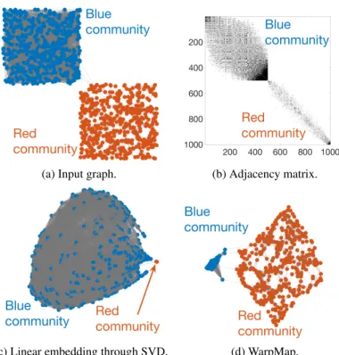
1.1 Our proposed graph embedding algorithm WarpMap introduces a warping function, which

significantly improves the quality of a graph embedding. We expect the nodes in the blue community should be close in proximity in the graph embedding domain because their

connections are strong, which is shown by WarpMap. . . 7

2.1 Multi-layer neural network model [1] . . . 13

2.2 Convolutional neural network model [1] . . . 14

2.3 Recurrent neural network model [2] . . . 14

2.4 Generative adverserial network (GAN) results from [64]. Note that both samples above are generated samples from a neural network, that is to say, none of the figures actually exist in the real world. All pictures are "created" or drawn via a Deep Generative Model, which is a GAN in this case. . . 16

2.5 Graphical model of the generative process in VAE [32] . . . 19

2.6 Generative Adversarial Network model . . . 21

2.7 RL environment settings . . . 23

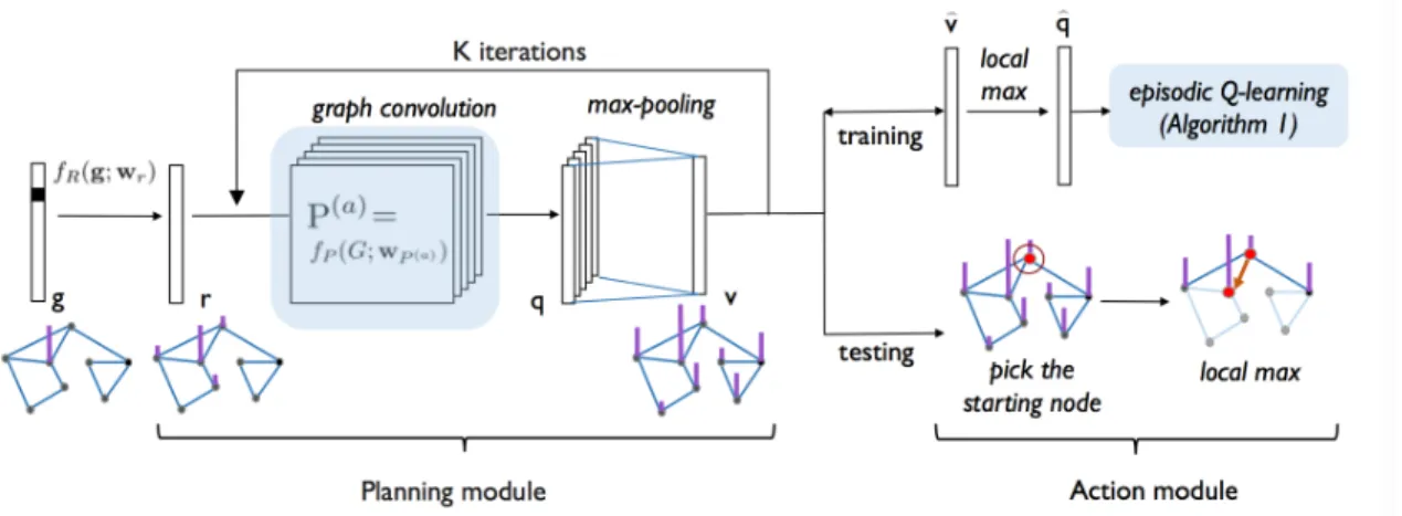
3.1 Architecture of GVIN. The left module emulates value iteration and obtains the state values; the right module is responsible for selecting an action based on an-greedy policy (for training) or a greed policy (for testing). We emphasize our contributions, including graph convolution operator and episodicQ-learning, in the blue blocks. . . 33

3.2 Matrix-vector multiplication as graph convolution. Through a graph convolution operatorP, r+γvdiffuses over the graph to obtain the action-value graph signalq. . . 36

3.3 The directional kernel function activates the areas around the reference directionθ`in the 2D spatial domain. The activated area is more concentrated whentincreases. . . 37

3.4 The spatial kernel function activates the areas around the reference directionθ`and reference distanced`in the 2D spatial domain. . . 38

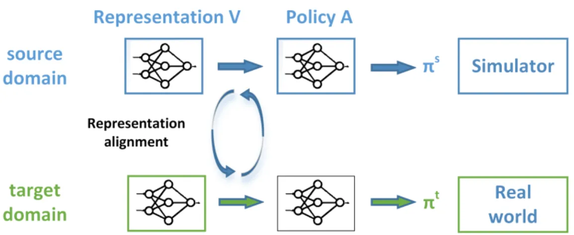
3.5 Problem setup illustration. The network with the blue bounding box represents the network trained in the source domain, while the green one represents the network running in the target domain. In our setup, the representation/perception module in target domain is pre-trained, while the parameters of policy module are unknown. . . 52

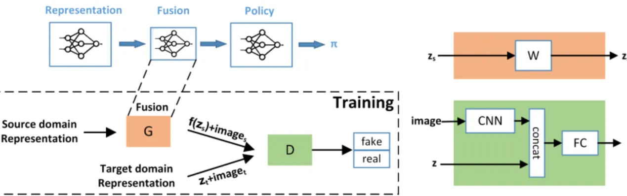
3.6 Fusion layer architecture and training. The fusion layer, which is a linear transformation, is inserted between the representation module and the policy module; the lower box shows the adversarial training setup for the fusion layer, described in Section 3.3.3; the right hand side of the figure shows the network architecture of the discriminator and mapping function (fusion layer). Implementation details are described in Section 5.3 . . . 54

5.1 Value map visualization on regular and irregular graph. . . 66

5.2 Q- vs. episodicQ-learning on16×16Maze. . . 66

5.3 Kernel direction order influences the planning performance in regular graphs (images). . . 67

5.4 Kernel direction order influences the planning performance in irregular graphs. . . 69

5.6 Sample planning trajectories on Minnesota highway map. . . 71 5.7 Sample planning trajectories on New York City street map. . . 71 5.8 The defaulted setting for the walk length is the diameter of input graph. The walk length

influences the classification performance. An empirical choice of walk length is the diameter of input graph (Kaggle 1968 and BlogCatalog [132]). . . 74

5.9 Walk memory does not matter. Walk memory factors do not significantly influence the

classification performance (Kaggle 1968). . . 75 5.10 Warping matters. Nonlinearity significantly influences the F1 score (Blogcatalog). The

warping function normalizes the distribution of all elements in the proximity matrix; when the distribution is symmetric (skewness is zero), the best performance is achieved. . . 76 5.11 Symmetry matters. A symmetric distribution of elements ing−1(Π)optimizes the empirical

performance (BlogCatalog). . . 77 5.12 In the dataset of Kaggle1968, the number of steps and nonlinear significantly influence the

classification performance. . . 78 5.13 WarpMap outperforms competition. The closed-form WarpMap (uw, grey diamond) is the

most accurate; scalable WarpMap (s-uw, red) is much faster than DeepWalk (dw, blue) and node2vec (n2v, yellow). . . 80 5.14 Thelogfactor amplifies small discrepancies. Plot(a)considers a linear warping function

g(x) =g−1_{(x) =x; Plot(b)considers an exponential warping functiong(x) =exp(x)and} g−1_{(x) =log(x). . . . 81} 5.15 WarpMap scales linearly. The proposed algorithm WarpMap scales well, linearly with the

number of edges. (U.S. patent 1975–1999 dataset; see Lemma 5.) . . . 82 5.16 t-SNE visualization on CIFAR-10 for different training senarios. the red is from source domain,

and the green one comes from target domain.Left: the visualization of source domain feature and target domain feature before alignment. Middle: the aligned feature embedding use Vanilla AL. We mark the corresponding CIFAR label on each cluster group based on most appeared classes.Right: the aligned feature embedding use WAL+CNN. . . 83 5.17 New imitation learning network in CARLA. The image module consists of 8 CNN and 2 FCN.

The speed feature is generated from 2 FCN. The policy module consists of 3 FCN that process the feature concatenated from image and speed. . . 85 5.18 Environment samples from three different domains in CARLA . . . 86 5.19 The mapping from source domain to taret domain in CARLA. . . 87 5.20 Source domain image samples and its corresponding aligned target domain images. The first

and third rows are sunset environment images (source domain), the second and fourth rows are nearest neighbor images in the rainy environment (target domain). . . 87

Chapter 1

Introduction

Over the past decade, the digital revolution has enabled vast amounts of data to be accessible. Massive amounts of data created by social media and scientific/engineering applications open new doors for analyzing economic value, unearthing scientific truth, and improving customer services. Data processing and data analysis have become a crucial challenge. Research in academia and industry is mainly concentrated on how to extract knowledge from big data using techniques including Machine Learning, data mining, operational research, etc [3, 96, 93].

Machine Learning is the study of how to design a machine that can learn from data. Industry leaders have invested significant effort into mining latent information from available data via machine learning techniques. However, traditional machine learning capabilities have reached an upper bound, even after increasing the scale of datasets. In general, Machine Learning is categorized as Supervised Learning, Unsupervised Learning, and Reinforcement Learning (RL). Supervised Learning algorithms analyze the training data and infers a function mapping to predict unseen instances. Unsupervised Learning finds hidden structure in unlabeled data, such as clustering, dimensional reduction, feature extraction and so on. RL is concerned with how an agent should react in an environment so that the agent can maximize accumulated rewards.

A methodology known as Deep Learning has emerged as a promising research area that outper-forms state-of-the-art published results and approaches human-level performance in several applications. Deep learning is positioned for a promising future in Big Data analytics, allowing computational models composed of a multitude of processing layers to learn representations of data through several levels of ab-straction. Deep learning has achieved tremendous success in numerous supervised learning tasks, including

speech recognition [5, 106], object recognition [51, 127, 72], semantic segmentation [98], natural language processing [122, 55, 73] and much more.

Reinforcement learning (RL) is a learning technique that solves sequential decision making problems that lack explicit rules and labels [124]. Recent developments in Deep Reinforcement Learning (DRL) have lead to enormous progress in autonomous driving [13], innovation in robot control [78], and human-level performance in both Atari games [87, 48] and the board game Go [115]. Given a reinforcement learning task, the agent explores the underlying Markov Decision Process (MDP) [11, 12] and attempts to learn a mapping of high-dimensional state space data to an optimal policy that maximizes the expected return.

In this thesis, we are specially interested in the Deep Reinforcement Learning (DRL) technique, which introduces Deep Learning into Reinforcement Learning settings. Conventional RL use tabular representation to hold the model information, whereas DRL uses neural networks as a function approximator to backup the policy information. Under the theory of RL, one of the important factors is whether the agent has access to (or learns) a model of the environment. By the model, we mean the function of state transitions and rewards. Algorithms that use a model are called model-based RL and those that do not are called model-free RL. If the agent knows the model beforehand, the agent could plan ahead, which means see what would happen in the future and decide among multiple choices. However, in practice, the true model of the environment is not available to the agent. In this case, the agent must learn the model from the sampled data, which is also called system identification. The biggest drawback is that the learned model often is often biased or inaccurate, resulting an agent policy that is optimized on the learned model and behaves sub-optimally.

On the other hand, model-free RL is more popular in the DRL community since they are easier to implement and do not encounter the model compounded error issue found in model-based RL. The samples from policy are unbiased true experiences, which are used to update the policy network. Typically, there are three approaches to train the agent by using model-free RL: policy-based, value-based, and actor-critic. The policy-based and actor-critic methods are usually on-policy learning, meaning that the sampled data is directly used to train the current policy function. Value-based methods, such asQ-learning or Deep Deterministic Policy Gradient (DDPG), are usually off-policy learning, that is learning current policy by using the samples from other policies, such as old policy [88] or expert’s policy [56]. In practice, on-policy learning normally provides more stable training, whereas off-policy reuse data more effectively, offering better sample efficiency.

1.1

Dissertation Research

Even though model-free RL has been popular in the research community and shows great success in variety of applications, recent researchers [61, 82] show that the current DRL approach is not a path towards Artifical General Intelligence (AGI). In the following, we list limitations from a variety perspectives:

• Model-free RL shows poor sample efficiency: the task of RL aims to maximize the accumulated rewards. In most applications, reward signals are very sparse, such that when a policy search is conducted on the parameter space, most of time the agent receives no feedback at all. In other words, it is hard to track any gradient information during optimization since the policy is searching a Kronecker delta function. Therefore, the agent spends most of the sampled trajectories doing random search, which is highly inefficient. Additionally, DRL becomes worse when employing a neural network as the function approximator: current Deep Learning is inherently data hungry, that is deep learning requires large-scale datasets with high-quality labels even in supervised learning settings.

• Model-free RL is hard to train: When using a neural network as a non-linear function approximator, the convergence of a model-free RL algorithm cannot be guaranteed theoretically. A comparison is shown in Table 1.1. The main reason that RL is difficult to train is that it is a multi-level optimization problem. The inner loop optimizes the policy to maximize the total returns and the outer loop optimize the parameters of the policy network to minimize the gradient loss.

On/Off-Policy Algorithm Table Lookup Linear Non-Linear

MC ! ! ! On-Policy TD(0) ! ! 7 TD(λ) ! ! 7 MC ! ! ! Off-Policy TD(0) ! 7 7 TD(λ) ! 7 7

Table 1.1: Algorithm Convergence [125]

• Model-free RL shows poor generalization: [63] shows that even a tiny visual differences or envi-ronment variations could lead to total failure of a state-of-the-art model-free DRL. The model-free DRL makes no assumption about the domain structures since the deep neural network system is simply memorizing the mapping relationships between inputs and outputs, thus it is capable of highly limited generalization, reasoning, and planning capabilities.

• Model-based RL has inherent problem of modeling errors: The advantage of model-based RL is that it improves the sample efficiency compared with a model-free RL. However, the model-based method requires system identification step to map the observations to a dynamics model. Then, a learned model is used to solve the policy. In many applications, such as robotic manipulation and locomotion, accurate system identification is difficult, and modelling errors can severely degrade the policy performance.

• DRL has a reality gap issue: The pre-assumption of RL is that the agent is designed to interact with the environment, and in many business applications, it is too expensive or even impossible for an agent to interact with hypothetical trial and error scenarios. For example, training an autonomous car in the real world might damage the car or hit the pedestrian. The central question is how to solve this reality gap issue. That is, how to effectively transfer a policy learned in a simulator to the real world.

The aforementioned limitations are also current active research topics. Methods such as Hindsight Experience Replay (HER) [6], model-based RL [116], and planning algorithms [94] are proposed to solve the sample efficiency. The combination of model-based RL and model-free RL [145, 116] could further improve the compound error of learned environment dynamics. Meta learning [34] and planning [94, 128] could effectively generalize to environment variants. Also, transfer learning and meta learning provide the possibility to transfer the learned knowledge from a simulator to the real world.

1.2

Methods of Study

Among these limitations and their corresponding research proposals, one question remains: what is the fundamental problem behind these drawbacks? And is there an universal approach to solving the above problems that shares the same properties? Further, we think this is also one of the key factors towards AGI. The central theme among the above problems is that state-of-the-art deep learning models lack, ironically, a ’model’ from which to learn: when humans begin solve a complicated task, he or she often first builds a world knowledge or ’model’ in his or her mind, then performs inference or planning upon that model. The model can be naturally represented as a graph. The graph is a discrete data structure model of the instance relationships. Unlike current deep learning systems, which learn the function mapping between two variables, a graphical model takes consideration of the dependencies among latent variables, the relationships among the latent variables essentially forms the conditional probability or potential function, which is already widely used

in the probabilistic graphical model (PGM) [69]. However, the inference in PGM is commonly intractable, using different approximation or reduction techniques. On the other hand, a neural network introduces a fully differentiable method to do inference based on backpropagation in a convenient way. Then, it is natural to combine the graphical model and neural network together to model the dependencies, while using a neural network for inference task.

Additionally, the reality gap is a typical problem of domain transfer/adaption. Ideally, we are interested in learning adaption with a set of unlabeled source examples and a set of unlabeled target examples. The goal is to find or construct a common representation space for the two domains. One possible way is by using adversarial learning methods [45], which learn feature representations from samples in different domains that are indistinguishable.

According to this analysis, our research can be abstracted as three sub-tasks:

• Dynamic graph planning based on neural networks: Here dynamic means the graph contains un-known dynamics, for example, traffic on the map, or network bandwidth state on network routing. The graph can be viewed as a semi-model and the model transition probability remains unknown. Therefore, we explore a RL model between model-free and model-based.

• Graph embedding: In the previous bullet, we assume that the graph structure features are given a priori. Our research investigates how to obtain the structure features from the raw graph for a variety of tasks including control, classification, clustering, etc.

• Domain adaption between different environments: How to bridge the gap between RL training in a simulator to a real world environment without any supervision signal. Also, for practical reason, our interests also lie on the domain transfer with light computational cost.

1.2.1

Dynamic graph planning based on neural networks

RL can be categorized as model-free [80, 86, 87] and model-based approaches [124, 30, 108]. Model-free approaches learn the policy directly by trial-and-error and attempt to avoid bias caused by a suboptimal environment model [124]. Model-based approaches, on the other hand, allow for an agent to explicitly learn the mechanisms of an environment, which can lead to strong generalization abilities. A recent work, the value iteration networks (VIN) [128] combines recurrent convolutional neural networks and max-pooling to emulate the process of value iteration [11, 12]. As VIN learns an environment, it can plan shortest paths for unseen mazes.

The input data fed into deep learning systems is usually associated with regular structures. For example, speech signals and natural language have an underlying 1D sequential structure; images have an underlying 2D lattice structure. To take advantage of this regularly structured data, deep learning uses a series of basic operations defined for the regular domain, such as convolution and uniform pooling. However, not all data is contained in regular structures. In urban science, traffic information is associated with road networks; in neuroscience, brain activity is associated with brain connectivity networks; in social sciences, users’ profile information is associated with social networks. To learn from data with irregular structure, some recent works have extended the lattice structure to general graphs [29, 68] and redefined convolution and pooling operations on graphs; however, most works only evaluate data that has both a fixed and given graph. In addition, most lack the ability to generalize to new, unseen environments.

In this subsection of research, we aim to enable an agent to self-learn and plan the optimal path in new, unseen spatial graphs by using model-based DRL and graph-based techniques. This task is relevant to many real-world applications, such as route planning of self-driving cars and web crawling/navigation. The proposed method is more general than classical DRL, extending for irregular structures. Furthermore, the proposed method is scalable (computational complexity is proportional to the number of edges in the testing graph), handles various edge weight settings and adaptively learns the environment model. Note that the optimal path can be self-defined, and is not necessarily the shortest one. Additionally, the proposed work differs from conventional planning algorithms; for example, Dijkstra’s algorithm requires a known model, while our proposed method aims to learn a general model via trial and error, then apply said model to new, unseen irregular graphs.

1.2.2

Graph embedding

A graph embedding is a collection of feature vectors associated with nodes in a graph; each feature vector describes the overall role of the corresponding node. Through a graph embedding as shown in Figure 1.1, we are able to visualize a graph in a 2D/3D space and transform problems from a non-Euclidean space to a Euclidean space, where numerous machine learning and data mining tools can be applied. The applications of graph embedding include graph visualization [54], graph clustering [141], node classification [111, 151], link prediction [79, 8], recommendation [148], anomaly detection [4], and many others. A desirable graph embedding algorithm should (1) work for various types of graphs, including directed, undirected, weighted, unweighted and bipartite; (2) preserve the symmetry between the graph node domain and the graph embedding domain, that is, when two nodes are close/far away in the graph node domain, their corresponding embeddings

are close/far away in the graph embedding domain; (3) be scalable to large graphs; and (4) be interpretable, that is, we understand the role of each building block in the graph embedding algorithm.

(a) Input graph. (b) Adjacency matrix.

(c) Linear embedding through SVD. (d) WarpMap.

Figure 1.1: Our proposed graph embedding algorithm WarpMap introduces a warping function, which significantly improves the quality of a graph embedding. We expect the nodes in the blue community should be close in proximity in the graph embedding domain because their connections are strong, which is shown by WarpMap.

1.2.3

Domain adaption between different environments

Most DRL [87, 80, 74, 35] studies are conducted in a simulated environment from scratch. Training an agent in a real world environment is often too expensive or even unrealistic. An alternative is to apply the model learned from the simulator to the real world. However, directly adopting the model trained from the simulator to a real physical system commonly leads to poor performance. How to perform transfer from simulation to the real world plays a key role in robotics since the simulator can be a source of practically infinite cheap data with flawless labels.

Since multiple factors could contribute to performance degradation from the simulator to the real world, we summarize from the macro-view as two main points: 1) the mismatch of perception or sensory feature representation and 2) the policy bias that is caused by mismatched dynamics between the simulator

and real environment.

The model of the agent can be partitioned as two parts: the representation module and the policy module. The representation module performs feature extraction, and the policy module could be either model-free or model-based [124]. Many recent efforts in RL domain transfer [129] focus on the policy transfer, where their applications simplify state by using low dimensional sensor input data such as IMU. On the other hand, most of the work regarding representation transfer [136, 14] in RL settings attempts to learn the generator function to adapt the images from the source domain to appear as possible to those sampled from the target domain. However, this method is relatively cumbersome and it is typically specific to robotics.

As [113] demonstrated, good representation allows a trained policy to be quickly adapted and recovered even when the policy network is obliterated. The robust representation greatly eases the learning difficulties when performing domain transfer in RL problems. In this research, we propose to develop an adversarial learning for the feature-level domain transfer, in which the features from the source domain can be aligned to the target domain without any labels. Particularly, our work mainly focuses on image-based input for the agent since the real world environment largely involves image-based state and the computer vision community already provides large amounts of data and advanced neural network based models for image classification [51], object detection [101, 51], and segmentation [22].

1.3

Contributions and Outline

The reminder of this dissertation is organized as follows: Chapter 2 provides background information related to Machine Learning, deep generative model, and RL. Chapter 3 presents the details and design architectures of the aforementioned three sub-taskes including GVIN, WarpMap graph embedding, and domain alignment based on adversarial learning. Chapter 4 presents literature review and related state-of-the-art work. Chapter 5 presents experiments and results, which we studies the empirical results and offers the corresponding analysis. Note that this chapter is also divided into three parts, each of them corresponding to one task in Chapter 3. Finally, conclusions and future work are discussed in Chapter 6.

Chapter 2

Background

In this chapter, we will cover the background knowledge used in this thesis. Much of the work in this thesis is based on Deep Learning, and hence we introduce Deep Learning techniques that are widely used in supervised learning. We will also review the concept of Deep Generative Model and its extensions, which is used in the proposed domain alignment algorithms for visual based input (Section 3.3). Additionally, we will go through the reinforcement learning basics and related state-of-the-art techniques, which is used in GVIN (Section 3.1). Finally, we will talk about the graph convolutional neural network (GCNN) and its extensions that are used later in Sections 3.1 and 3.2

2.1

Deep Learning

Deep Learning or deep neural networks (DNN) have shown great success in a variety of applications including image processing [72], speech processing [58], natural language processing [140], control [116] problems and others. These tasks can be modeled as either supervised learning or unsupervised learning. In this subsection, we will discuss popular supervised learning techniques, a variety of neural network architectures, and the auto differentiable system such as Tensorflow [3] which has lead to the explosive growth of Deep Learning applications.

2.1.1

Supervised Learning

From the point of view of supervised learning, many practical problems can be simply formulated as a computing mapping functionf:X→Y, whereXis in the input space andY is in the output space. Here

we list several popular applications that fall into this mapping function framework:

• Image recognitionin image recognition,Xis the space of image andY represents object probability • Machine translationfor machine translation,Xis source language (ex: English) andY is the target

language (ex: German)

• Image captioningin image captioning,X is query image andY is corresponding caption of that image • Speech recognition in speech recognition, X represents the audio wave data andY indicates the

transcripts of the corresponding audio wave

• Question answeringin question answering application,Xdenotes the questions and stories andY is the answer

In supervised learning, all of the above tasks become searching for a function that can exactly or approximately map fromX toY. Concretely, we assume that we have a training set withnsamples

{<x1, y1>, ...,<xn, yn>}wherex1...n∈Xandy1..g.n∈Y, and each sample is independent and identically distributed (i.i.d.). Then, the learning process aims to search over the mapping functionf so thatfmaintains the consistent mapping among all<xi, yi>pairs. Hence, we define an objective/loss functionL(yˆi, yi)to measure how consistent it is among the training set, whereyˆirepresents the prediction fromf, andyidenotes the ground truth value. In the general case, the loss function can be defined as:

f∗=arg min

f E<x,y>L(f(x), y) (2.1)

wheref∗ is the optimal function configuration;L(⋅,⋅)represents the loss function; andyˆ=f(x) denotes the prediction. Equation 2.1 indicates that the goal is to find the configuration off to minimize the expected loss over the training sample. Across the machine learning community,f has a variety of hypotheses. For example, in the linear model,f=x⊺θ+and the configuration is parameterθ. In the decision tree model, f is a tree, and the configuration indicates how the tree is split based on the loss criteria. In a neural network, f is a multi-layer perceptron and the parameters of the perceptron represent the configuration.

Searching the parameters of the functionf is an optimization problem. Unfortunately, optimizing on Equation 2.1 often yields poor performance on different datasets, such as the testing set versus real world deployment. In other words, the optimizedf does notgeneralizeto all<x, y>pairs, which is often referred to as overfitting. In order to choose a generalized solution from the set of optimizedf configurations,

regularization techniques are introduced to overcome overfitting. Therefore, the Equation 2.1 is written as:

f∗=arg min

f E<x,y>[L(f(x), y)] +R(f) (2.2)

whereR(f)is a scalar value added to the original loss function. Regularization follows the principle of Occam’s razor: "Suppose there exist two explanations for an occurrence. In this case, the one that requires the least speculation is usually better". In Equation 2.2,R(f)measures the model complexity. During the optimization, the loss function balances the objective loss and model complexity.

Nevertheless, directly optimizing Equation 2.2 is not tractable since the optimization needs to operate on all sample data. Therefore, stochastic gradient descent (SGD) is introduced to make the optimization scalable. Then, Equation 2.3 is more practical for ML applications:

f∗=arg min f 1 N N ∑ i=1 L(f(xi), yi) +R(f) (2.3)

Several popular optimization methods for ML algorithms are provided in the following discussion. Linear RegressionAssuming we have a regression task such that the target label is a continuous valueY ∈ Rand input features aremdimensionX ∈Rm. The loss function uses the mean squared error

(MSE) between the predicted valueyˆand the target valuey, whereyˆ=θ⊺x+θ0. Assuming the model follows a Gaussian, which is L2 regularization, putting each piece together, we have:

θ∗=arg min θ 1 N N ∑ i=1 ∣∣θ⊺xi+θ0−yi∣∣2 ´¹¹¹¹¹¹¹¹¹¹¹¹¹¹¹¹¹¹¹¹¹¹¹¹¹¹¹¹¹¹¹¹¹¹¹¹¹¹¹¹¹¹¹¹¹¹¹¹¹¹¹¹¹¹¹¹¹¹¹¹¹¹¹¹¹¹¹¸¹¹¹¹¹¹¹¹¹¹¹¹¹¹¹¹¹¹¹¹¹¹¹¹¹¹¹¹¹¹¹¹¹¹¹¹¹¹¹¹¹¹¹¹¹¹¹¹¹¹¹¹¹¹¹¹¹¹¹¹¹¹¹¹¹¹¹¶ training objective +λ m ∑ j=0 ∣∣θj∣∣2 ´¹¹¹¹¹¹¹¹¹¹¹¹¹¹¹¹¹¹¹¹¸¹¹¹¹¹¹¹¹¹¹¹¹¹¹¹¹¹¹¹¹¶ regularization (2.4)

λis the coefficient that determines how much regularization effect should be added. Equation 2.4 is also called the ridge regression. When the feature exhibits the sparsity property, the model can use the Laplace prior, which is L1 regularization, and we could replace the term∑m_j=0∣∣θj∣∣2with∑mj=0∣∣θj∣∣. The optimization of linear regression has a closed form solution and can be solved in one-step byθ∗= (X⊺X)−1X⊺y.

Logistic RegressionLogistic regression is a classical model for solving the binary classification problem. ConsiderY to be a discrete value, specifically in Logistic regression it is a binary value{0,1}. The hypothesis isyˆ=_1+e−1φ(x)₎ andφ(x) =θ⊺x+θ0. To optimize the parameters of logistic regression, the loss

function contains binary cross-entropy as the objective function and L2 norm as regularization: θ∗=arg min θ 1 N N ∑ i=1 (−yi∗log ˆyi− (1−yi) ∗log(1−yˆi)) ´¹¹¹¹¹¹¹¹¹¹¹¹¹¹¹¹¹¹¹¹¹¹¹¹¹¹¹¹¹¹¹¹¹¹¹¹¹¹¹¹¹¹¹¹¹¹¹¹¹¹¹¹¹¹¹¹¹¹¹¹¹¹¹¹¹¹¹¹¹¹¹¹¹¹¹¹¹¹¹¹¹¹¹¹¹¹¹¹¹¹¹¹¹¹¹¹¹¹¹¹¹¹¹¹¹¹¹¹¹¹¹¹¹¹¹¹¹¹¹¹¹¹¹¹¹¹¹¹¹¹¹¹¹¹¹¹¹¹¹¹¸¹¹¹¹¹¹¹¹¹¹¹¹¹¹¹¹¹¹¹¹¹¹¹¹¹¹¹¹¹¹¹¹¹¹¹¹¹¹¹¹¹¹¹¹¹¹¹¹¹¹¹¹¹¹¹¹¹¹¹¹¹¹¹¹¹¹¹¹¹¹¹¹¹¹¹¹¹¹¹¹¹¹¹¹¹¹¹¹¹¹¹¹¹¹¹¹¹¹¹¹¹¹¹¹¹¹¹¹¹¹¹¹¹¹¹¹¹¹¹¹¹¹¹¹¹¹¹¹¹¹¹¹¹¹¹¹¹¹¹¶ training objective +λ m ∑ j=0 ∣∣θj∣∣2 ´¹¹¹¹¹¹¹¹¹¹¹¹¹¹¹¹¹¹¹¹¸¹¹¹¹¹¹¹¹¹¹¹¹¹¹¹¹¹¹¹¹¶ regularization (2.5)

The optimization uponθ, which we call training in later sections, uses SGD to update the parameter byθnew=θold−α∇L(θold), whereαis a hyper-parameter called the learning rate that defines the gradient step size in each iteration.

Support Vector Machine ClassificationConsider a binary classification problem with labelsyand featuresx. We will usey∈ {−1,1}to denote the class labels. Given each training sample<xi, yi>, SVM aims to find the optimal or robust decision boundary that maximize the geometric margins. Assuming the parameterθ= {w, b}, the loss function becomes a constrained optimization:

max w,b 1 2∣∣w∣∣ 2 s.t. yi(w⊺xi+b) ≥1, i=1, ..., m (2.6)

Typically, by using Lagrange duality, the above quadratic programming (Equation 2.6) can be eventually constructed as follows:

L(w, b) = 1 2∣∣w∣∣ 2 ´¹¹¹¹¹¹¹¸¹¹¹¹¹¹¶ regularization +C m ∑ i₌1 max(0,1−yi(w⊺xi+b)) ´¹¹¹¹¹¹¹¹¹¹¹¹¹¹¹¹¹¹¹¹¹¹¹¹¹¹¹¹¹¹¹¹¹¹¹¹¹¹¹¹¹¹¹¹¹¹¹¹¹¹¹¹¹¹¹¹¹¹¹¹¹¹¹¹¹¹¹¹¹¹¹¹¹¹¹¹¹¹¹¹¹¹¹¹¹¹¹¸¹¹¹¹¹¹¹¹¹¹¹¹¹¹¹¹¹¹¹¹¹¹¹¹¹¹¹¹¹¹¹¹¹¹¹¹¹¹¹¹¹¹¹¹¹¹¹¹¹¹¹¹¹¹¹¹¹¹¹¹¹¹¹¹¹¹¹¹¹¹¹¹¹¹¹¹¹¹¹¹¹¹¹¹¹¹¶ training objective (2.7)

The above loss function (Equation 2.7) is also called hinge loss. However, the operatormax(⋅,⋅)is not differentiable. The sub-gradient is computed to optimize the objective function.

Neural Network Classification Neural networks extend logistic regression to a more complex hypothesis. Logistic regression could be viewed as a special case of neural networks that contains one neuron output with a single layer. Neural networks stack multiple layers and we are free to choose from a variety of linearity activation functions including sigmoid, hyperbolic tangent tanh, rectifier relu, etc. The non-linearity enables neural networks with more powerful model expressiveness. [114] shows that a single layer of sigmoid or tanh functions is Turing-complete, which means the neural network can approximate arbitrary function mapping. Similarly, the loss function of the neural network could also be formed as Equation 2.3. However, with direct multi-layer optimization it is difficult to search the optimal parameters via SGD. The

Backpropagation algorithm allows the gradient to be passed back to the previous layer based on the chain rule, updating the neural network weights layer by layer. Therefore, Backpropagation enables the research community to train very large scale networks for a variety of applications, such as image processing, speech processing, text processing, etc.

2.1.2

Different Neural Architectures

Here we briefly show three basic and commonly used neural network architectures in different applications.

2.1.2.1 Multi-layer Neural Network

Figure 2.1: Multi-layer neural network model [1]

Multi-layer neural networks receive the input feature and transform it through a series of hidden layers. Each hidden layer is made up of a set of neurons, where the neurons in a single layer are completely independent (do not share connections) as shown in Figure 2.1. Each neuron is a linear transformation of the input features with non-linear activation. In a conventional multi-layer perceptron, the sigmoid is a popular activation function but recent models show that the sigmoid experiences a gradient vanishing problem and is therefore replaced with a rectifier function.

2.1.2.2 Convolutional Neural Network

Convolution neural networks (CNN) specifically handle the data that consists of the spatial invariant property, such as image, video, etc. Figure 2.2 shows an example of image data to illustrate its mechanism. The input color image is of size128×128×3(length and height are128,3color channels for rgb). The input image is convolved with CNN learned filters and each channel is independently computed. However, directly applying a fully connected neural network requires a very large number of parameters. Instead, CNN require

Figure 2.2: Convolutional neural network model [1]

two assumptions: 1) image data has local connectivity, that is the current pixel is only related to its local region of the input, and 2) the parameters in the sliding window is shared among the entire image. These two assumptions allow for a dramatic reduction in the number of parameters for CNN.

2.1.2.3 Recurrent Neural Network

Figure 2.3: Recurrent neural network model [2]

Many applications contain a sequence of data, such as time series, natural language, speech recogni-tion, etc. A recurrent neural network (RNN) shown in Figure 2.3 accepts input sequence{x1, ...xT}and has the feedback loop using a recurrence formulaht=f(ht−1, xt;θ). The parameterθis shared at every time step, allowing the network to process arbitrary sequence lengths. As shown in Figure 2.3, RNNs can be unfolded as a chained feed-forward neural network, which could potentially cause the gradient vanishing problem. In order to overcome the gradient drawbacks, long short term memory (LSTM) [59] and gated recurrent units (GRU) [25] utilize gating and memory to address the limitations. LSTM and GRU model are summarized as:

LSTM ft=σ(Wf[ht−1, xt] +bf) it=σ(Wi[ht−1, xt] +bi) ¯ Ct= tanh(WC[ht₋1, xt] +bC) Ct=ft∗Ct−1+it∗C¯t ot=σ(Wo[ht₋1, xt] +bo) ht=ot∗ tanh(Ct) GRU zt=σ(Wz[ht−1, xt]) rt=σ(Wr[ht₋1, xt]) ¯ ht= tanh(W[rt∗ht−1, xt]) ht= (1−zt) ∗ht₋1+zt∗¯ht

2.1.3

Auto Differentiable System

Neural networks provide an elegant way to train the deep network by the chain rule. It is natural to think about the neural network as a computational graph, which lead the research community to redefine the artificial neural network. The graph is not necessary limited to the bipartite graph, but rather it could be any directed acyclic graph (DAG) of operations: input feature vectors flow along edges and vertices which are differentiable operators, output flows out to another differentiable module or loss function. In the implementation, the vertices objects implement forward() and backward(⋅) function, where forward(⋅) function propagates the graph in topological order producing the prediction based on the network parameters, and backward() function passes the gradient from the next layer to the previous layer in reverse order. When vertices among the computational graph are connected, each gradient in the neuron are chained and training can be fully automated.

The computational graph concept is one of biggest reasons why Deep Learning has been such a significant achievement: 1) it allows developers to define neural networks in a modular fashion, where each module can be highly customized to specific problems; and 2) the developer does not need to derive backpropagation from scratch, many auto differentiable systems such as Tensorflow [3] and Pytorch [96] automate the backpropagation process for users.

2.2

Deep Generative Model

Often typical generative models consist of two types of variables: observed/visible variablexand latent/hidden variablesz. xis commonly pre-given during the training phase, where variablezis used to describe the structure inx.zdepends on the model parameters that are trained through the learning algorithms.

Generative models directly learn the data distribution which can be used in variety of scenarios. Figure 2.4 shows the result from a few samples generated from a generative adversarial network (GAN) [45]; note that every picture is generated via the neural network and the input is random noise.

Figure 2.4: Generative adverserial network (GAN) results from [64]. Note that both samples above are generated samples from a neural network, that is to say, none of the figures actually exist in the real world. All pictures are "created" or drawn via a Deep Generative Model, which is a GAN in this case.

We use the following notations:

• xrepresents an observed random variable

• p(x)represents the probability over the variablex

• X ∼p(x)denotes a valueXsampled from the probability distributionp(x); symbol∼denotes sampling • P(x)represents the density function of the distribution ofx

According to the Bayesian rule:

p(z∣x) = p(x∣z)p(z) p(x) =

p(x, z)

∫ p(x, z)dz (2.8)

where p(x∣z)is the likelihood, p(z)is the prior probability, p(z∣x)is the posterior probability, andp(x)is the evidence. Equation 2.8 represents how to perform an inference over the graphical model.

∫ p(x, z)dzintegrates all possible configurations over the latent variables, which is a NP-hard problem. To overcome the computational limitations, the research community proposes exact inference and approximate inference. Since we are mainly focused on the approximate inference approach, we omit background information for exact inference research.

Approximate inference could be divided into two types: Monte Carlo Markov Chain (MCMC) and variational inference. Instead of computing the true posterior distribution, MCMC constructs a markov chain to obtain samples of the desired distribution after a number of steps. While variational inference provides an approximation to the posterior based on known distribution. Since our research utilizes deep implicit density estimation (ex: GAN), we only discuss the variational inference and variational autoencoder that is currently popular among the Deep Learning domains.

2.2.1

Variational Inference

The posterior distributionp(z∣x)is often computationally intractable in many models and thereby we use a parametric distribution qφ(z∣x)such as a Gaussian to approximate the true distribution p(z∣x). Performing inference on the known distribution is computationally tractable, then our task has converted inference as an optimization problem where we train the parametersφso thatqis as close topas possible.

To measure the distance betweenqandp, variational inference uses the reverse KL Divergence:

KL(q∣∣p) = ∑

z

qφ(z∣x)log

qφ(z∣x)

p(z∣x) (2.9)

wherep(z∣x) = p_p(x,z_(x))is from Equation 2.8, then:

KL(q∣∣p) = ∑ z qφ(z∣x)log qφ(z∣x)p(x) p(z, x) = ∑ z qφ(z∣x)(log qφ(z∣x) p(z, x) +logp(z)) = (∑ z qφ(z∣x)log qφ(z∣x) p(z, x)) + (∑z logp(x)qφ(z∣x)) = (∑ z qφ(z∣x)log qφ(z∣x) p(z, x)) + (logp(x) ∑_z qφ(z∣x)) = (∑ z qφ(z∣x)log qφ(z∣x) p(z, x)) +logp(x) (2.10)

∑zqφ(z∣x)log qφ(z∣x)

p(z,x) sincelogp(x)is fixed. Therefore, the objective function becomes:

∑ z qφ(z∣x)log qφ(z∣x) p(z, x) =Ez∼qφ(z∣x)[log qφ(z∣x) p(z, x)] =Ez_∼qφ(z∣x)[logqφ(z∣x) −logp(z, x)]

=Ez∼qφ(z∣x)[logqφ(z∣x) −logp(x∣z) −logp(z)] (2.11)

Here, minimizing the above equation is equivalent to maximizing:

maxL =Ez_∼qφ(z∣x)[−logqφ(z∣x) +logp(x∣z) +logp(z)] =Ez∼qφ(z∣x)[logp(x∣z) +log

p(z) qφ(z∣x)]

(2.12)

whereLis variational evidence lower bound (ELBO), which is computationally feasible since we can evaluatep(x∣z),p(z)andq(z∣x). The ELBO could be reformulated as:

L =Ez_∼qφ(z∣x)[logp(x∣z) +log

p(z) qφ(z∣x)]

=Ez∼qφ(z∣x)[logp(x∣z)] −KL(Q(z∣x)∣∣P(z)) (2.13)

In another point of view, when substitutingLback to Equation 2.9, we have:

KL(q∣∣p) =logp(x) − L

logp(x) = L +KL(q∣∣p) (2.14)

wherelogp(x)is the log likelihood of true data distribution and it remains constant over the parame-tersφ. Therefore, to minimize the KL divergenceKL(q∣∣p)asKL(q∣∣p) ≥0is equivalent to maximizingL. In summary, the variational inference intends to optimize the following objective function:

Figure 2.5: Graphical model of the generative process in VAE [32]

2.2.2

Variational Auto-Encoder

Variational auto encoder (VAE) [67] provides an elegant amortized inference approach extended from the variational inference. VAE use two neural networks to parameterize the variational parameters φand generative processθ, where the graphical model is shown in Figure 2.5. Therefore, we rewrite the Equation 2.15 as follows for the optimization objective function:

L(x;θ, φ) =Ez∼qφ(z∣x)[logpθ(x∣z)] −KL(Qφ(z∣x)∣∣Pθ(z)) (2.16)

The first termEz∼qφ(z∣x)[logpθ(x∣z)]denotes the log likelihood that the Auto-Encoder can be used

for reconstruction loss, where the second term is the regularization term. It describes that by using an arbitrarily high capacity model forq(z∣x), we adjustq(z∣x)to actually matchp(z∣x); the KL-divergence term becomes zero when the perfect match.

TheKL(Qφ(z∣x)∣∣Pθ(z)term is not analytically formed for computation. In practice, we assume bothQφ(z∣x)andPθ(z)are two Gaussian distributions. Then the problem becomes a density estimation to infer the Gaussian parameters. Neural networks can be viewed as a powerful function approximator, therefore we can combine a simple distribution with a learned neural network to emulate an arbitrary distribution.

Therefore, the prior distribution could be set asN (0, I), whereIis the identity matrix. For each latent Gaussian, the latent dimension could be inkdimension. To simplify the assumption, VAE assumes that each latent dimension is independent, where the covariance matrix is a diagonal matrix.

closed form as follows:

KL[Qφ(z∣x)∣∣Pθ(z)] = ∫ qφ(z∣x)(logpθ(z) −logqφ(z∣x))dz

= 1₂ΣJ_j=1(1+log((σj)2) − (µj)2− (σj)2) (2.17) where written in matrix form as follows:

KL[N (µ(x),Σ(x))∣∣N (0, I)] =1

2(tr(Σ(x) + (µ(x))

⊺_{(µ(x))) −k−log det(Σ(x))) (2.18)}

After we have the analytic computation form (Equation 2.18), the loss function in Equation 2.16 can be iteratively trained via the stochastic gradient descent algorithm. And VAE can fit into the Auto-encoder framework, whereqφis the encoder andpθis the decoder.

However, one typical problem in VAE is that the sampling process is non-differentiable. To overcome the gradient estimation issue, [67] introduces a reparameterization trick: converting the sampling process to a differentiable operator as follows:

z=µ(x) +∗Σ(x)where∼ N (0, I) (2.19)

Equation 2.19 is equivalent to z ∼ N (µ(x),Σ(x)) and is widely used for continuous random variables. In the case of categorical distribution, Gumbel-softmax [62] can be adopted, which shares a similar idea as continuous variables. Assuming that each categorical variable probability isπi, to draw the samplez, the reparameterization trick becomes:

z= one_hot(arg max

i [gi+logπi]) (2.20)

wheregiis the noisegi∼ Gumbel(0,1). Then, the VAE is fully differentiable in both continuous variables and discrete variables, and thereby could be directly trained based on the backpropagation algorithm.

2.2.3

Generative Adversarial Learning

VAE is an explicit density estimation where the latent distribution is a Gaussian distribution. Gen-erative adversarial network (GAN) [45] is a recently proposed implicit density estimation method. Unlike the variational inference, which uses another distribution (ex: Gaussian) to approximate the posterior, GAN does not contain any explicit probability distributions, but instead, using one neural network to mimic any data distribution while another one to evaluate the distribution quality. The generator defines a process to simulate data and does not require tractable densities.

Figure 2.6: Generative Adversarial Network model

As shown in Figure 2.6, the GAN model consists of two neural networks: generator and discriminator. The input to the generator is from a simple prior, which could be a high dimensional vector generated from a random uniform distribution. To evaluate the generated samples, instead of using likelihood to evaluate the generator, GAN utilizes another neural network (discriminator) to measure how good the sample is. This becomes a two player game for implicit density estimation, where two networks are optimizing opposite objectives. The overall loss function is:

min

G maxD V(D, G) (2.21)

where:

V(D, G) =_Ex_∼pdata(x)[logD(x;θD)] +Ez∼pz(z)[log(1−D(G(z;θG);θD))] (2.22)

pz(z)is the prior distribution, which could be set asN (0, I). Equation 2.22 is a standard binary cross entropy loss when training a standard binary classifier with a sigmoid output. However, compared with

conventional classifier, the framework takes two minibatches of data where one is from the true distribution and the other one is from the generator. The intuition is that the discriminator tries to distinguish between the real data and generated one, whereas the generator tries to fool the discriminator that it cannot distinguish between them. The cost used for the discriminator is:

J(D)(θD, θG) = − 1

2Ex∼pdata(x)[logD(x;θD)] − 1

2Ez∼pz(z)[log(1−D(G(z;θG);θD))] (2.23)

The generator and discriminator are parameterized throughθGandθD. During the training phase, the generator and discriminator are learned iteratively. At each step, a minibatch ofxvalues from the true dataset and a minibatch of azvalues drawn from the generator’s prior over latent variables are sampled, and then two stochastic gradient descent (SGD) steps are applied: one updatingθDby minimizingJ(D)and the other updatingθGby maximizingJ(D).

However, the Equation 2.23 is mainly used for theoretical analysis. In practical applications, the gradient of the generator could quickly vanish when the discriminator rejects the fake samples. One common improvement modifies the generator loss function as follows:

J(G)= −1

2Ez∼pz(z)[logD(G(z;θG);θD)] (2.24)

A further improvement is to do maximum likelihood learning with GANs in practice as follows:

J(G)= −1

2Ez∼pz(z)[e

σ−1(D(G(z;θG);θD))] _(2.25)

whereσdenotes the logistic sigmoid function.

State-of-the-art GAN research [7, 47, 64, 18] mainly focuses on two points: 1) how to produce the sample as realistic as possible and 2) how to stabilize the GAN training process and also avoid the mode collapse issue. Mode collapse represents the generator collapses, which produce limited modes and sample variety. We will discuss state-of-the-art approaches that overcome these drawbacks in Section 4.

Compared with results from VAE, which often produce blurry samples, GAN generates more sharp and realistic samples. Many researchers believe that the effect comes from the VAE minimizing the asymmetric divergence (ex: KL divergence) between the data and the model, whereas the GAN minimizes the Jensen-Shannon (JS) divergence, which is symmetric. Some clues [44] show that even using different divergence,

the model still encounters the sample quality, training stability, and mode collapse problems. Therefore, specifically why GAN produces more realistic samples is still not clear to the current research community.

2.3

Reinforcement Learning

Figure 2.7: RL environment settings

Reinforcement learning (RL) is primarily used to solve the sequential decision making problem, which is also a typical control problem. Compared with supervised learning or unsupervised learning that collects large amounts of data for training, RL (shown in Figure 2.7) requires an interactive query in the environment to learn the optimal policy, which is maximizing the accumulated rewards. The learning process was originally inspired from neuro-psychology.

Unlike conventional control methodology which uses domain knowledge to build a mathematical model of the system dynamics, RL is a data-driven approach to learn the optimal policy. In the conventional optimal control, we have:

minEe[ΣTt=1Ct(xt, ut)] (2.26)

s.t. xt+1=ft(xt, ut, et),

ut=πt(τt)

whereCt(xt, ut)is the user defined cost,ftdenotes the state transition function,τt= (u1, ..., ut−1, x0, ..., xt) represents an observed trajectory,etis the noise process, andπt(τt)is the optimization decision variable. Typically, the state transition is unknown and the system identification is employed to learn continuous system dynamics.

utis the action at each step, andCt(xt, ut)denotes the reward function. Unlike traditional control methods, which use a model driven approach, RL is a data driven method that learns optimal policy from the data. RL follows the Markov Decision Process (MDP) or Partially Observable Markov Decision Process (POMDP). In this research, we mainly focus on problems that are modeled by MDP, therefore we omit discussion of POMDP.

2.3.1

Markov Decision Process

We consider an environment defined as an MDP<S, A,Ps′,s,a,Rs,a, γ>that contains a set of states

s ∈ S, a set of actionsa∈ A, a reward functionRs,a, and a series of transition probabilitiesPs′,s,a, the probability of moving from the current statesto the next states′given an actiona. The goal of an MDP is to find a policy that maximizes the expected return (accumulated rewards):

Rt= ∞

∑

k₌0

γkrt+k (2.27)

wherert+kis the immediate reward at the(t+k)th time stamp andγ∈ (0,1]is the discount rate. A policyπa,sis the probability of taking actionawhen in states. The value of statesunder a policyπ,vπs, is the expected return when starting insand followingπ; that is,vπ_s =E[Rt∣St=s]. The value of taking action

ain statesunder a policyπ,qπ_s(a), is the expected return when starting ins, taking the actionaand following π; that is,qπ(_sa)=E[Rt∣St=s, At=a]. A policy is defined as:

π(s) ∶S→A (2.28)

The value-function is used to estimate how good it is at statest. If the agent uses a given policyπ, the corresponding value-function can be written as:

Vπ(s) =Eπ[ T−1

∑

k=0

γkrk] (2.29)

Among all possible value-functions, there exists an optimal value function that is higher than others for all states:

V∗(s) =max π V

π₍

and the optimal policy is:

π∗(s) =arg max π V

π_(s)

(2.31)

RL also introduces an additional value function (action-value function) to evaluate at specific states, the value of agent applying specific action. The action-value function, also calledQfunction, is a function of the state-action paired with real values, where mathematicallyQ:S×A→_R. The optimalQfunction, which is defined asQ∗(s, a), has the following relationship with optimal value functionV∗(s):

V∗(s) =max a Q

∗_{(s, a) (2.32)}

and is similar to the value function. If we know the optimalQfunction, the optimal policy chooses the action that gives maximumQ∗(s, a):

π∗(s) =arg max a Q

π_{(s, a)}

(2.33)

2.3.2

Dynamic Programming

The typical way to update theQfunction andV function is based on the Bellman Equation, which uses dynamic programming to recursively update the value function.

Q∗(s, a) =R(s, a) +γ ∑ s′∈S p(s′∣s, a)V∗(s′) (2.34) where: V∗(s) =max a Q ∗_{(s, a) (2.35)}

In summary, for the value-based RL, there is always at least one policy that is better than or equal to all other policies, called an optimal policyπ∗; that is, the optimal policy isπ∗=arg maxπvπs, the optimal state-value function isv∗_s=maxπvsπ, and the optimal action-value function isq∗(

a)

s =maxπqπ(sa). To obtain

π∗andv∗, we usually consider solving the Equations 2.34 and 2.35.

Policy iteration and Value iteration are two popular dynamic programming algorithms to solve the Bellman equation in the discrete state space.

Value iterationThe algorithm initializes V(s)to random values, then we iteratively compute vs←maxa∑s′Ps′,s,a(Rs,a+γvs′)until the result converges. The algorithm is guaranteed to converge to the

Algorithm 1Value Iteration

1: InitializeV(s)with random value

2: repeat 3: for alls∈Sdo 4: foralla∈Ado 5: Q(s, a) ←R(s, a) +γ∑s′_∈Sp(s′∣s, a)V(s′) 6: end for 7: V(s) ←maxaQ(s, a) 8: end for 9: untilV(s)converge

optimal values [125] and the algorithm is given in Algorithm 1:

Policy iterationThe goal of the agent is to obtain the optimal policy. Therefore, instead of repeatedly improving the value-function, policy iteration updates policy in each epoch and the value is re-computed upon the new policy. The policy iteration is also guaranteed to converge to the optimal policy and normally takes less iteration than the value iteration algorithm. The detailed algorithm in shown in Algorithm 2

Algorithm 2Policy Iteration

1: Initialize policyπ′randomly

2: repeat 3: π←π′ 4: Improve values: 5: Vπ(s) ←R(s, π(s)) +γ∑s′∈Sp(s′∣s, π(s))Vπ(s′) 6: Improve policy: 7: π′(s) ←arg maxa(R(s, a) +γ∑s′∈Sp(s′∣s, a)Vπ(s′)) 8: untilπ=π′

The challenge to use policy iteration and value iteration is that both algorithms assume the agent knows the environment dynamics (p(s′∣s, a)) beforehand. However, this is often not true in most applications. One possible approach to this issue is to use system identification, which is similar to traditional control methods. Another alternative is to use model-free RL techniques. Model-free RL can be categorized as three types: value-based, policy-based, and actor-critic.

2.3.3

Value-based Model-free RL

Q-learning is to approximate the state-action pairs Q-function from the samples that the agent observes during the interaction with environment. Since Equation 2.34 still requires the model dynamics p(s′∣s, a),Q-learning uses the Bellman equation to learn directly theQvalues from the data. The update rule

can be written as:

Q(s, a) =R(s, a) +γmax a′ Q(s

′_{, a}′_{) (2.36)}

Therefore the policy becomesa=arg maxaQ(s, a). Nevertheless, the agent should not greedily choose the optimal policy at the initial stage, but rather explore the environment. Hence, the-greedy algorithm balances the exploration and exploitation during training. The trade-off between exploration and exploitation belongs to the study of the bandit problem. We do not discuss the more advanced methods such as the Thompson Sampling and Upper Confidence Bound (UCB) since they are out of scope of this research.

DeepQNetwork (DQN) [88] uses a neural network to approximate theQfunction. However, using a nonlinear approximator forQ-learning does not guarantee convergence. To stabilize the training, DQN introduces the experience replay buffer and target network. The loss function is defined as:

L(θ) = 1

2∑_i ∣∣R+γmaxa′ Qθ(s ′

i, a′i) −Qθ(si, ai)∣∣22 (2.37)

where each<si, ai, s′i, ri>are sampled from the experience replay buffer. The experience replay buffer collects history policy of the neural network. In other words, the current policy is updated by old policy or another policy. Then, this is a typical off-policy learning. The experience replay buffer provides better sample efficiency, that is, the agent repeatedly samples from historical data to correct the currentQfunction. Also, the experience replay buffer could be flexible and filled with other policies, for example, the optimal trajectory or high quality policy.

DQN also introduces the target network. In Equation 2.37, the termR+γmax′_aQθ(s′i, a′i)shifts in every iteration, which falls into the feedback loop between the target and estimatedQ-value. In other words, the value estimations can easily spiral out of control. The target network employs the secondQnetwork that fixes the network’s weights and only periodically or slowly updates it from the primaryQ-network. Therefore, the new loss function can be written as:

L(θ) = 1

2∑_i ∣∣R+γmaxa′ Qˆθ(s ′

i, a′i) −Qθ(si, ai)∣∣22 (2.38)

2.3.4

Policy Optimization

In the policy gradient approach, instead of using the value function to estimate expected returns from some policy, the agent directly uses the function approximator to map input state to action. Recall that the goal of RL ismax_Eπ[R], whereR=r0+r1+...+rT−1, the agent must solve the gradient of the objectives. Consider a general expectation_Ex∼p(x∣θ)[f(x)], the gradient is:

∇θL(θ) = ∇θEx∼p(x∣θ)[f(x)] = ∇θ∫ p(x∣θ)f(x)dx = ∫ ∇θp(x∣θ)f(x)dx = ∫ p(x∣θ)∇θp(x∣θ) p(x∣θ) f(x)dx = ∫ p(x∣θ)∇θlogp(x∣θ)f(x)dx =Ex_∼p₍x_∣θ₎[∇θlogp(x∣θ)f(x)] (2.39)

we replace thef(x)to be the accumulated rewardsR, andp(x∣θ)to be the policy networkπ(at∣st, θ). Then, the policy gradient can be written as:

∇θEπ[R] =Eπ[ T−1 ∑ t₌0∇ θlogπ(at∣st, θ) T−1 ∑ t′=t γt′−trt′] (2.40)

Equation 2.40 is the famous REINFORCE algorithm [126]. However, the vanilla REINFORCE is a high variance and unbiased gradient estimator, which could take many long iterations for the algorithm to converge. One typical approach is to add the baseline termb(s) =E[rt+γrt+1+γ2rt+2...+γT−1−trT−1]as:

∇θEπ[R] =Eπ[ T−1 ∑ t=0 ∇θlogπ(at∣st, θ)( T−1 ∑ t′=t γt′−trt′−b(st))] (2.41)

since expectation ofb(s)is also unbiased, that isEπ[∑Tt=−01∇θlogπ(at∣st, θ)b(s)] =0, the conclu-sion is easy to prove and thereby we omit it here. For simplicity, the termAˆt= (Rt−b(st))is also called the advantage function, whereRt= ∑Tt′−₌t1γt

′_−t

rt′and Equation 2.41 can be written as:

∇θEπ[R] =Eπ[ T−1

∑

t=0