Matrix-Vector Nonnegative Tensor Factorization for
Blind Unmixing of Hyperspectral Imagery
Yuntao Qian,
Member, IEEE
, Fengchao Xiong, Shan Zeng, Jun Zhou,
Senior Member, IEEE
, and
Yuan Yan Tang,
Fellow, IEEE
Abstract—Many spectral unmixing approaches ranging from geometry, algebra to statistics have been proposed, in which nonnegative matrix factorization (NMF) based ones form an important family. The original NMF based unmixing algorithm loses the spectral and spatial information between mixed pixels when stacking the spectral responses of the pixels into an observed matrix. Therefore, various constrained NMF methods are developed to impose spectral structure, spatial structure, and spectral-spatial joint structure into NMF to enforce the estimated endmembers and abundances preserve these structures. Com-pared with matrix format, the third-order tensor is more natural to represent a hyperspectral data cube as a whole, by which the intrinsic structure of hyperspectral imagery can be losslessly retained. Extended from NMF based methods, a matrix-vector nonnegative tensor factorization (NTF) model is proposed in this paper for spectral unmixing. Different from widely used tensor factorization models such as Canonical Polyadic decomposition (CPD) and Tucker decomposition, the proposed method is derived from block term decomposition (BTD) which is a combination of CPD and Tucker decomposition. This leads to a more flexible frame to model various application-dependent problems. The matrix-vector NTF decomposes a third-order tensor into the sum of several component tensors, with each component tensor being the outer product of a vector (endmember) and a matrix (corresponding abundances). From a formal perspective, this tensor decomposition is consistent with linear spectral mixture model. From an informative perspective, the structures within spatial domain, within spectral domain, and cross spectral-spatial domain are retreated inter-dependently. Experiments demonstrate that the proposed method has outperformed several state-of-the-art NMF based unmixing methods.
Index Terms—Hyperspectral imagery, Spectral unmixing, Ten-sor factorization, Spectral-spatial structure
I. INTRODUCTION
Hyperspectral imagery (HSI) has drawn much attention from various applications. It provides information about both spectral and spatial distributions of distinct objects owing to its numerous and continuous spectral bands. In an HSI, each pixel represents the spectral irradiance of the corresponding
This work was supported by the National Natural Science Foundation of China 61571393, 61303116, 61273244, the Research Grants of University of Macau MYRG2015-00049-FST, MYRG2015-00050-FST, the Science and Technology Development Fund of Macau 026-2013-A, the Australian Re-search Councils DECRA Projects funding scheme DE120102948.
Y. Qian and F. Xiong are with the Institute of Artificial Intelligence, College of Computer Science, Zhejiang University, Hangzhou 310027, P.R. China. ([email protected])
S. Zeng is with the College of Mathematics and Computer Science, Wuhan Polytechnic University, Wuhan 430023, P.R.China.
J. Zhou is with the School of Information and Communication Technology, Griffith University, Nathan, Australia
Y. Y. Tang is with the Faculty of Science and Technology, University of Macau, Macau 999078, China.
object materials. Due to limited spatial resolution of HSI and complicated material constitution, a pixel often covers several different materials. Therefore, the spectral irradiance is a com-bined outcome of several materials according to their distribu-tions and configuradistribu-tions, leading to the existence of “mixed” spectra in some pixels. Hence, hyperspectral unmixing, which decomposes a mixed pixel into a collection of constituent spectra, or endmembers, and their corresponding fractional abundances, becomes an important task for hyperspectral data analysis.
Many hyperspectral unmixing methods have been proposed, ranging from geometry, algebra to statistics [1], [2]. Most of them are based on linear spectral mixture model, i.e., the spectrum of a pixel is a linear combination of endmembers with corresponding abundances. If pure pixels are assumed to exist in an HSI, convex geometry based approaches such as Pixel Purity Index (PPI) [3], N-FINDR [4], and vertex component analysis (VCA) [5], to name just a few, are used to estimate endmembers. However, in many cases such assumption is not met or pure pixels have been contaminated by various factors from environment and devices. Minimum volume based algorithms [6] can partly tackle this problem. In other cases, if the endmembers in an HSI are known in advance or a library of spectral signatures including all endmembers in the HSI can be obtained, fully constrained least-squares (FCLS) [7] and sparse regression algorithms [8] can be used. If very little prior knowledge is available, unmixing can be considered as a blind source separation (BSS) problem from the statistics perspective [2], [9]–[11]. Among a number of BSS methods, nonnegative matrix factorization (NMF) and its variations have been widely used due to its clear physical, statistical, and geometric interpretation, flexible modeling, and less requirement on prior information [12], [13]. NMF usually provides a part-based representation of data, i.e., NMF based spectral unmixing decomposes an HSI into two nonnegative matrices that represent fractional abundances and spectral endmembers respectively. Though effective, however, NMF faces some difficulties in real applications. The solution space of NMF is always very large, which, added to the fact that the cost function is also not convex, makes the algorithm prone to noise corruption and computationally demanding. To reduce solution space, extensions of NMF including symmetric NMF, semi-NMF, convex NMF, and multi-layer NMF have been proposed [14]. More recently, sparse NMF assumes that most of the pixels are the mixtures of only a small number of endmembers [15]–[17]. This implies that a number of entries in the abundance map are zeros or very small. In the literature,
L0, L1, and L1/2 norms have all been utilized to define the sparsity constraint.
Another problem of NMF based methods is the loss of spatial location information when unfolding an HSI cube into a matrix, i.e., the spectral signatures of pixels are stacked as rows in this matrix, so that the spatial positions of pixels cannot be fully preserved in the row indices. Furthermore, the relations between the spatial and spectral domains are also deteriorated. To address this problem, various constrained NMF models are proposed [13], [18]–[21]. In [13], sparse NMF with piecewise smoothness constraint was proposed, in which the piecewise smoothness of endmember signatures and abundance fractions was embedded into NMF to overcome their discontinuity and noise. In [18], a spatial similarity constraint was added into NMF, by which the abundance of a pixel was promoted to be consistent with the average abundance of its surrounding pixels. To make use of the spectral-spatial joint information, Mei et al [19] presented a neighborhood preserving regularization approach that was based on the assumption that each pixel could be linearly reconstructed by its spatial neighboring pixels. This regulariza-tion was added into NMF to keep the local geometric structure of HSI. Lu et al [20] assumed that pixels with similar spectral signatures often imply similar abundances with respect to the given endmembers, leading to a manifold regularizer based NMF. Wang et al [21] constructed a hypergraph to accurately capture the spectral-spatial joint structure of HSI, and added this hypergraph to NMF as a constraint. These approaches not only address the lacking of structural information of NMF, but also improve the stability of matrix decomposition and the robustness to noises. However, under matrix factorization framework, the spectral and spatial structures are employed by adding the corresponding constraints into NMF model, which is not straightforward and is not able to convey a complete HSI structure.
To overcome the limits of NMF and constrained NMF, extending matrix factorization to tensor factorization is a potential way. An HSI data cube can be represented as a third-order tensor without any information loss, therefore compared with matrix factorization based unmixing methods, tensor factorization is a more natural and structural model. Tensors (or way arrays) are highly suitable for multi-dimensional data such as HSI, video, social network, array signal, and so on [22]. Tensor analysis methods, especially the models and efficient algorithms for tensor decompositions, have been extensively studied and applied to many real-world problems ranging from psychometrics and chemometrics to signal processing, computer vision, neuroscience, and data mining [23]–[26]. In the field of HSI processing and analysis, tensor decompositions have been used for data compres-sion [27], [28], denoising [29]–[31], feature extraction [32], change detection [33], [34] and classification [35], [36]. All these approaches use a low-rank tensor representation to approximate the original HSI data. The low-rank tensor representation can reduce memory storages, remove noises, and extract discriminative features. Among them, Canonical Polyadic decomposition (CPD) and Tucker decomposition (or called higher-order singular value decomposition) are two
widely-used tensor factorization models.
To our best knowledge, the research on tensor factoriza-tion based spectral unmixing is relatively under explored. In 2007, Zhang et al [37] applied tensor factorization to spectral unmixing for the first time, and then they published a more comprehensive paper [38] on tensor based HSI data analysis for a space object material identification study including unmixing problem. In their method, nonnegative CPD firstly decomposes a tensor into a sum of component rank-one tensors, then these rank-one tensors are grouped by clustering method according to their similarity. Finally, the rank-one tensors in each group are combined to form an endmember and its corresponding abundances. Following this work, Huck et al [39] proposed that nonnegative Tucker decomposition also could unmix hyperspectral data. From then on, the studies on tensor factorization based unmixing seldom appear. Recently, the use of compression-based nonnegative CPD to analyze HSI data in temporal series or in multi-angular acquisitions was presented [40], [41]. In this approach, a third-order tensor is used to represent several related HSI data sets with one of its modes denoting the time/angle dimension, i.e., each HSI cube is still represented by matrix. In [42], a new tensor based nonlinear mixing model was presented, which extended the existing bilinear mixing models to an infinite number of reflections. However, the tensor was used to represent the multilinear interaction among materials and multiple light scattering effects, but not for describing the spectral-spatial structure of HSI.
As we know, HSI data compression, dimension reduction, feature extraction and noise removal mainly focus on da-ta reconstruction with minimal error, but spectral unmixing pays more attention to whether the decomposed factors are consistent with the physical mechanism of mixing process. Whichever CPD or Tucker decomposition based unmixing algorithm is used, its link with linear mixing spectral model is not as explicit as that of matrix factorization. The CPD based rank of a tensor is defined as the minimum of rank-one tensors that are summed to express this tensor, but this tensor rank cannot be considered as the number of endmembers, which makes the endmember detection and the corresponding abun-dance estimation to be not easy. For Tucker decomposition based algorithm, the spectral mode rank can be directly equal to the number of endmembers, but orthogonality between the components does not conform to the characteristics of endmembers. Moreover, the strong interaction between modes in Tucker decomposition destroys the properties of part-based representation and nonnegativity in linear spectral mixture model. Therefore, it is necessary to develop an effective and explicit technique to apply tensor factorization for spectral unmixing.
Under tensor notation, the linear spectral mixture model can be rewritten so that an HSI data tensor is approximated by sum of the outer products of an endmember (vector) and its corresponding abundance map (matrix). This form of tensor factorization exactly corresponds to matrix-vector (slab-fiber) third-order tensor factorization which decomposes a tensor into a sum of component tensors, and each component tensor is a matrix-vector outer product. The matrix-vector third-order
tensor factorization can be seen as a specific case of block term decompositions (BTD) [43]–[45]. BTD is a combination of CPD and Tucker decomposition. It decomposes a tensor into a sum of component tensors as CPD, while each component tensor is factorized as Tucker decomposition. BTD overcomes the limit of CPD that each of its component tensor must be rank-one, meanwhile it lifts the restriction of Tucker decomposition that there is just one component tensor. BTD provides a flexible frame to construct tensor decomposition models according to their application-dependent physical inter-pretation. The matrix-vector third-order tensor decomposition lets each component tensor be an outer product of a vector (an endmember) and a matrix (the corresponding abundance map), by which we construct a straightforward link between tensor decomposition and linear spectral mixture model. Therefore, this type of tensor factorization has explicit physical inter-pretation under the assumption of linear spectral mixture, as well as preserves a complete spectral-spatial structure without any information loss. In this paper, we propose a matrix-vector nonnegative tensor factorization (NTF) based spectral unmixing method, give its solving algorithm, and discuss its distinct properties. The main contribution of our work is cleaning off some very pivotal obstacles when tensor methods walks into spectral unmixing application.
The rest of the paper is organized as follows. In Section II, we briefly introduce the linear spectral mixture model and the background of tensor factorization. This section emphatically analyzes the limitation of existing tensor-based unmixing algorithms and leads to the matrix-vector tensor factorization. In section III, the model and algorithm of matrix-vector NTF based spectral unmixing are described in detail, and the uniqueness of model and the convergence of optimization are also discussed. Results on the synthetic and real-world data are reported in Sections IV. Finally, Section V draws conclusions and suggests future research.
II. BACKGROUND AND MOTIVATION
Unmixing aims at detecting the existence of the contributing materials in a scene and estimating their proportions. To do so, the mixing/unmixing models are crucial, which should consider the interpretation of the image formation process, be physically meaningful, statistically accurate, and compu-tationally feasible. In this section, we introduce the linear spectral mixing model and its link with tensor decompositions. In particular, we give the motivation behind the matrix-vector tensor decomposition based unmixing method.
A. Notations and concepts
In this paper, scalars are denoted by lowercase letter, e.g.,
x, vectors are written in boldface lowercased, e.g.,x, matrices correspond to boldface capitals, e.g.,X, and high-order tensors (order three or higher) are denoted by Euler script letters, e.g.,
X. A matrix is a second-order tensor, a vector is a first-order tensor, and a scalar is a tensor of order zero. A tensor can be represented as a multidimensional array of numerical values. In this representation, the elements in a k-th order tensor are identified by a k-tuple of subscripts, e.g.,xi1,i2,...,ik. The
operations upon tensor is based on multilinear algebra. Some important operations and concepts of matrix and tensor that are used in this paper are listed here, and the others are introduced later when they appear.
Definition 1: Different dimensions of an array are called modes. A matrix has two modes (column mode and row mode), and akth-order tensorXhask modes.
Definition 2:A tensor fiber is a one-dimensional fragment of a tensor, obtained by fixing all indices except for one.
Definition 3: A tensor slab is a two dimensional section (fragment) of a tensor, obtained by fixing all indices except for two indices.
Definition 4:Unfolding a tensor is the process of reordering the elements of akth-order tensor into a matrix. For a third-order tensor X∈RI×J×K, three matrices unfolded from this
tensor are defined by
(XJ K×I)(j−1)K+k,i = xijk (1) (XKI×J)(k−1)I+i,j = xijk (2) (XIJ×K)(i−1)J+j,k = xijk (3) Definition 5: Given two matrices A ∈ RI×J and B ∈ RK×L, their Kronecker product is a matrix denoted as A⊗
B∈RIK×J L and is defined as A⊗B= a11B a12B · · · a1JB a21B a22B · · · a2JB .. . ... . .. ... aI1B aI2B · · · aIJB (4)
Definition 6:The Khatri-Rao product of two matricesA∈ RI×J andB∈RK×J with the same number of columnsJ is
a matrix denoted asAB∈RIK×J and is defined as
AB= a1⊗b1 a2⊗b2 · · · aJ⊗bJ
(5)
Definition 7:Thek-mode (matrix) product of a tensorX∈ RI1,I2,...,IK with a matrixA∈
RJ×Ik is denoted byX×
kA
and is of sizeI1× · · ·Ik−1×J×Ik+1× · · ·IK. The elements
of this product are
(X×kA)i1···ik−1jik+1···iK =
Ik
X
ik=1
xi1i2···iKajik (6)
Definition 8: The outer product of two tensors A ∈ RI1×I2×...×IP andB∈RJ1×J2×...×JQ is the tensor A◦B∈ RI1×I2×...×IP×J1×J2×...×JQ and its elements are defined by
(A◦B)i1i2...iPj1j2...jQ=ai1i2...iPbj1j2...jQ (7) For example, the outer product of a matrixAand a vectorb is a third-order tensor.
B. Linear spectral mixture model
The linear mixture model represents the spectrum of a pixel of K wavelength-indexed bands in the observed scene based upon R endmembers and their corresponding abundances. It is given by
x=Ms+υ (8) wherexdenotes aK×1vector of the observed pixel spectrum in an HSI, s is a R×1 vector of abundance fractions for
each endmember, υ is a K×1 vector of an additive noise representing the measurement errors, and M is a K ×R
spectrum matrix whose columns correspond to an endmember spectrum.
Using matrix notation, the mixing model above for the N
pixels in the image can be rewritten as
X=MS+ Υ (9) where the matrices X∈RK×N,S∈
RR×N andΥ∈RK×N
represent, respectively, hyperspectral data, the abundances of all pixels on all endmembers, and additive noise.
Two properties are usually added to the linear spectral mixed model. The first is nonnegativity which assumes that the contribution from endmembers should be larger than or equal to zero, and the spectral irradiance of any material is also nonnegative, i.e., the matricesM andSare nonnegative. The second is sum-to-one ofswhich assumes that the proportional contributions from the endmembers to every mixed pixel should be added up to one.
C. The link between linear spectral mixture model and tensor factorization
Equation (9) can be seen as a matrix factorization problem. Many matrix factorization based unmixing algorithms have been proposed. The main trend of this family of approaches is to incorporate physical and mathematical constraints into matrix factorization models. Among these constraints, various spatial and spectral structures such as local and nonlocal similarity have been proved to be very helpful [19]–[21]. How-ever, these constraints cannot fully and accurately compensate for the structure loss during HSI to 2D matrix conversion. Tensor is a natural extension of matrix to represent multi-dimensional arrays. Obviously, the third-order tensor is a lossless representation of an HSI, which directly embeds the inherent spectral-spatial structure of an HSI into its own struc-ture and operations. In theory, it provides a more consistent and comprehensive framework for unmixing problem against matrix based methods.
Similar to matrix factorization which is an important tool of linear algebra for two-dimensional data analysis, tensor factorization is used to analyze the intrinsic/hidden structure of multi-dimensional array with multi-linear algebra. Here we briefly introduce two widely adopted and foundational tensor factorization methods, CPD and Tucker decomposition, and their applications to spectral unmixing.
Definition 9: The CPD factorizes a tensor into a sum of component rank-one tensors. For example, the CPD of a third-order tensor X∈RI×J×K is defined as
X=
R
X
r=1
ωr(ar◦br◦cr) (10)
The CPD for a third-order tensor is illustrated in Fig. 1(a).
Definition 10:The rank of a tensorXis the minimal number of rank-one tensors that yield X in a linear combination. A
kth-order tensor is a rank-one tensor if and only if it equals
the outer product of k nonzero vectors. The factor matrices associated with the CPD in Equation (10) can be expressed as A = [a1, . . . ,aR]∈RI×R (11)
B = [b1, . . . ,bR]∈RJ×R (12)
C = [c1, . . . ,cR]∈RK×R (13)
so that Equation (10) can be equivalently written in the form of unfolded matrices
XIJ×K = (AB)CT (14)
One can observe that Equation (14) and the linear spectral mixture model under matrix notation in Equation (9) seem to be identical in form without the noise term, i.e., (AB)
is a matrix with the size of IJ ×R representing the abun-dances of all pixels on all endmembers, andCT contains the
endmembers.
Definition 11:The Tucker decomposition factorizes a tensor to the k-mode product of a small core tensor and factor ma-trices. For example, given a third-order tensor X∈RI×J×K,
find a core tensor G ∈ RQ×T×V with the indices Q I, T J, and V K, and three factor matrices: A = [a1,a2, . . . ,aQ] ∈ RI×Q, B = [b1,b2, . . . ,bT] ∈ RJ×T, andC= [c1,c2, . . . ,cV]∈RK×V, so that X= Q X q=1 T X t=1 V X v=1 gqtv(aq◦bt◦cv) (15)
which also can be expressed in a compact matrix form using mode-k multiplications
X=G×1A×2B×3C (16)
Equation (16) can be equivalently unfolded as
XIJ×K = [(A⊗B)GQT×V]CT (17)
The Tucker decomposition for a third-order tensor is illus-trated in Fig. 1(b). We find that Equations (17) and (9) are also similar in form, i.e.,[(A⊗B)GQT×V]is a matrix with
the size of IJ×R representing the abundances of all pixels on all endmembers, andCT is the endmembers.
However, compared with matrix factorization, from the view of physical interpretation, the link between tensor decomposi-tion and linear spectral mixture model is still not clear. Fur-thermore, there are a lot of difficulties in the implementation of these two tensor factorization algorithms for unmixing. CPD based unmixing method requires the a priori knowledge of the tensor rank R. There is no straightforward algorithm to determine the rank of a given tensor. In fact, this is an NP-hard problem. In most cases, the number of endmembers can be obtained by means of statistical/geometrical methods or domain knowledge, but this estimated number of endmembers can not be used as tensor rank because it is much smaller than the real rank. In practice, for simplicity, max(I, J, L)
or its severalfold value is used as the tensor rank R in CPD. Consequently, each column of C is not identified as an endmember as in NMF based unmixing methods. In [37] it is assumed that a group of similar columns in C match to the same material so that the average or central vector of
a group can represent an endmember, and the corresponding abundance matrix of this endmember is the summation of the columns of AB in the same group. The groups are generated by clustering method. Although the mathematical justification of this assumption is not very solid, the exper-imental results on synthetic hyperspectral data sets reported in [38] are promising. However, it has been not applied to real HSI data. On the other hand, Tucker decomposition is a high order extension of singular value decomposition (SVD) of matrix. Firstly, SVD is not a suitable matrix decomposition for unmixing problem because its main property, orthogonality, does not match the physical mechanism of spectral mixing, i.e., the spectra of endmembers or abundance matrices in an HSI are not orthogonal to each other. Secondly, the core tensor
G is related to all three mode factors A, B andC, but how to divideGinto abundance and endmember respectively is not straightforward and its physical mechanism remains uncertain. Thirdly, the nonnegative property of mixture model is not easy to be imposed on Tucker decomposition. Hence, Tucker decomposition based unmixing method is more difficult to interpret than CPD based method [39].
A main difference between CPD and Tucker decompositions is that CPD treats all tensor modes equally and processes them identically while Tucker decomposition can distinguishes the modes of tensor according to their application-dependent phys-ical interpretation. Although an HSI can be represented and processed as a third-order tensor, its modes are distinguishable in the spectral-spatial manner, in which two spatial indices are distinguished from a spectral mode. On the other hand, Tucker decomposition does not clearly divide a tensor into a sum of a set of component tensors, so that it is difficult to directly link it to the linear mixture model. Fortunately, several groups of researchers have proposed models that combine aspects of CPD and Tucker [22]. Among them, block term decompo-sitions (BTD) is a typical one for modelling more complex tensor structures than CPD and Tucker decomposition [43], [44].
Definition 12: The BTD factorizes a tensor into a sum of component tensors (or called terms), and each component tensor is defined as the k-mode product of the core tensor and factor matrices. For example, given a third-order tensor
X∈RI×J×K, X= R X r=1 Gr×1Ar×2Br×3Cr (18)
The BTD for a third-order tensor is illustrated in Fig. 1(c). Compared with CPD, it does not require that each component tensor is rank-one. Compared with Tucker decomposition, it is a sum of several component tensors rather than just one. Therefore, BTD is the generalization of CPD and Tucker decomposition, which has been used for decoupling mul-tivariate polynomials [46], blind deconvoluting DS-CDMA signals [47], separating mixed audio signal, and so on [45].
According to linear spectral mixture model, it is expected that an HSI tensor can be approximated by a sum of com-ponent tensors in which each comcom-ponent tensor is the outer product of a matrix and a vector (endmember). This matrix
represents abundances of corresponding endmember at each pixel. As the spatial position information of pixels is kept in this matrix, it is also called abundance map. To this end, we only need to set Gr ∈ RLr×Lr×1 to be an identity matrix, Ar ∈ RI×Lr, B
r ∈ RJ×Lr, and c
r ∈ RK×1, leading to a
specific BTD.
Definition 13:The matrix-vector tensor decomposition fac-torizes a third-order tensor into a sum of component tensors. Each component tensor is defined as the outer product of a matrix Er and a vector cr, and Er is the product of two
matricesAr andBr. X= R X r=1 Ar·BTr ◦cr= R X r=1 Er◦cr (19)
The matrix-vector tensor decomposition is illustrated in Fig. 1(d), which is also named as BTD in rank-(Lr, Lr,1) terms.
CPD is a specific BTD with rank-(1,1,1)terms.
For matrix-vector tensor decomposition based unmixing,cr
can be considered as therth endmember andEr is the
corre-sponding abundance map. Now a straightforward link between matrix-vector tensor decomposition and linear spectral mixture model has been set up.
III. MATRIX-VECTORNONNEGATIVETENSOR
FACTORIZATION BASEDUNMIXING MODEL
In the last section, we have built a link between matrix-vector tensor factorization and linear spectral mixture model on their form of representation. However, the same form between them cannot guarantee that the endmembers and abundances of all the materials could be recovered by such ten-sor decomposition. Therefore, besides the same factorization form, matrix/tensor factorization should add some physical mechanism based conditions to make the result fit in a specific goal. Among them, nonnegativity based factorization solution is attractive because it usually provides a part-based repre-sentation of the data, making the decomposition factors more intuitive and interpretable. In particular, part-based represen-tation strongly agrees with the physical mechanism of spectral mixture. The effectiveness of NMF based unmixing has been demonstrated in many published literatures [12], [13], [18]– [20]. Inspired by NMF based unmixing, we add nonnegativity into matrix-vector tensor factorization. Nonnegativity enables the tensor decomposition to be a part-based representation as NMF, leading the factorization result to meet the requirement of spectral unmixing.
Combining matrix-vertex tensor factorization and nonneg-ativity property, a spectral unmixing model under tensor notation can be derived.
X= R X r=1 Er◦cr+N= R X r=1 Ar·BTr ◦Cr+N s.t. Ar,Br,cr0 (20)
We call it the matrix-vertex NTF based unmixing model, in which X ∈ RI,J,K is a third-order HSI tensor with the
spatial size of I×J and the number of spectral bands K, cr is considered as an endmember, and the matrixEr as its
(a) CPD
(b) Tucker decomposition
(c) BTD
(d) Matrix-Vector tensor decomposition Fig. 1. Four tensor decomposition models of a third-order tensor.
If the noise termNis ignored, the matrix representation of Equation (20) can be written as
XIJ×K = [(A1B1)1L1· · ·(ARBR)1LR]·C T (21) XJ K×I = (B¯C)·AT (22) XKI×J = (C¯A)·BT (23) in which A = [A1. . .AR], B = [B1. . .BR], and C = [c1. . .cR].1Lr is an all-one column vector with lengthLr.
Definition 14:The operation¯ is a generalized Khatri-Rao product for partitioned matrices with the same number of
sub-matrices. For example, both matrices Aand B haveR sub-matrices, so their generalized Khatri-Rao product is defined as
A¯B= (A1⊗B1. . .AR⊗BR) (24)
The matrix-vector NTF based unmixing is to estimate cr
andEr,r= 1, . . . , R, which can be defined as an optimization
problem of minimizing the mean square error (MSE) with nonnegative constraints min E,ckX− R X r=1 Er◦crk2F s.t. Ar,Br,cr0 (25)
in which Frobenius norm of a third-order tensor is defined as
kXkF = s X i X j X k x2 ijk (26)
Alternating least square minimization algorithm is used to solve this optimization problem [48], [49], i.e., the cost function is minimized in an alternating way for each factor matrix while the others are fixed. If we fix B and C, the sub-optimization problem is min A kXJ K×I−(B ¯ C)·ATk2 F s.t. A0 (27)
We deduce the multiplicative update rule using the method of Lagrange multipliers. Let S = B¯C, and the Lagrange functionΨis given by
Ψ =kXJ K×I−S·ATk2F + ΘA (28)
Taking the partial derivatives ofΨwith respect toA, we get
∇AΨ = (SAT −XJ K×I)TS+ Θ (29)
According to the Karush-Kuhn-Tucker (KKT) conditions,
ΘA=0, the multiplicative update rule forA is obtained. A←A.∗XTJ K×IS./(ASTS) (30) Similarly, the sub-optimization problem and its multiplicative update rule forB are
min B kXKI×J−(C ¯ A)·BTkF2 s.t. B0 (31) B←B.∗XTKI×JS./(BSTS) (32) whereS=C¯A.
The sub-optimization problem and the multiplicative update rule forC are
min C kXIJ×K−[(A1B1)1L1· · ·(ARBR)1LR]·C Tk2 F s.t. C0 (33) C←C.∗XTIJ×KS./(CSTS) (34) whereS= [(A1B1)1L1· · ·(ARBR)1LR].
The alternating least square optimization algorithm for Equation (25) is shown in Algorithm 1. Step 4 is used to avoid the overflow or underflow of A and B during computation process of Algorithm 1.
Algorithm 1 Alternating least square algorithm for matrix-vector NTF
Input: An HSI cube (third-order tensor)X
Parameters R,Lr, r= 1, . . . , R. For simplicity, Lr=L
for allr.
Output: A,B, andC.
1: InitializeA,B andC.
2: UpdateAwith Equation (30)
3: UpdateB with Equation (32)
4: Column scaling ofA andB.
A:,i←A:,i/kA:,ik,B:,i←B:,i· kA:,ik 5: UpdateC with Equation (34)
6: Repeat steps 2-5 until convergence of the cost function in Equation (25).
The number of endmembers R can be determined a prior by domain knowledge or endmember extraction methods [50], [51].
Lr is an important parameter, which controls the rank of
abundance matrix of the rth endmember. As we know the rank of Er = Ar· BTr is not always equal to parameter Lr where Lr ≤min(I, J). Instead, the rank of Er must be
equal to or less than Lr, because the rank of the product of
two matrices is less than the smaller rank of these two factor matrices, and the rank of Ar or Br is also equal to or less
thanLr. Therefore, in theoryLr is only required to be equal
to or larger than the actual rank of abundance matrixErand is
equal to or less thanmin(I, J). However, from the perspective of implementation, closer value of Lr and the actual rank of
Er leads to more stable and accurate results of optimization,
because the sizes ofArandBr(number of variables need to
be estimated) become small when Lrapproximates the actual
rank of abundance matrix. In practice, accurate determination of the rank of abundance matrix Er of therth endmember is
impossible. We only know this matrix has low-rank or sparse property in most real cases due to its spatial correlation and sparse distribution. On the other hand, in general the ranks of the all abundance matrices Er for r= 1,2, . . . , Rare not
the same, so determination of these ranks is a more difficult task. Therefore, we can assign a relative small value to Lr
compared with I and J. For simplicity, Lr is set the same
value for r = 1, . . . , R. In the experiments, we will analyze the unmixing performance with respect to different values of
Lr.
The convergence of the cost function in Equation (25) is easy to prove. The cost functions in Equations (27), (31) and (33) are non-increasing under the update rules (30), (32), and (34) respectively, which has been proved in the convergence analysis of NMF algorithm with multiplicative update rules [52], as their update rules are identical. Obvi-ously, iteratively using these update rules, the cost function in Equation (25) will converge to a point and then cease to decrease.
Moreover, the uniqueness of matrix-vector NTF is also an interesting probelm. In [49], several conditions are giv-en, under which essential uniqueness of BTD with
rank-(Lr, Lr,1)or rank-(L, L,1)terms is guaranteed. For example,
one condition of them for BTD with rank-(L, L,1) terms
is that min(I, J) ≥ LR and C does not have proportional columns. This condition is sometimes satisfied for spectral unmixing in application. The number of endmembers R is limited, and the rank of abundance matrix L is less than the length I or width J of the image due to the assumption that the abundance map can be low-rank represented, so that
min(I, J) ≥ LR may be satisfied. At the same time there is not any pair of endmembers whose spectra are totally the same but only have scaling difference, which means there is not any pair of columns of C being proportional. Although by now a strict condition to guarantee the uniqueness of the proposed matrix-vector NTF has not been derived, i.e., nonnegative BTD with rank-(L, L,1) terms, some research works have shown that the conditions of uniqueness for a specific tensor decomposition can be relaxed to its nonnegative version [53]. Therefore, the uniqueness of matrix-vector NTF can be achieved in some cases of spectral unmixing.
No matter whether the uniqueness exists or not, the final solution of the optimal problem in Equation (25) based on alternating minimization technique and multiplicative update rule is dependent on the initialization due to its non-convex property. Random initialization is usually used, in which A, B and C are initialized by setting their entries to random values in the interval[0,1]. However, it does not well control the quality of the final unmixing result. In some methods, an alternative unmixing approach is selected to generate the initialized result [13], [21], which guarantees an acceptable final unmixing result. In this paper, in order to objectively eval-uate the performance of matrix-vector NTF algorithm without introducing external factors, we use random initialization for the experiments, and ten times are run to generate an average result for any experiment.
Besides the nonnegativity constraint, sum-to-one property is also widely considered. As the method proposed in [16], [21] for NMF based unmixing model, the sum-to-one constraint can be embedded into the matrix-vector NTF model in a similar way, therefore, the cost function in Equation (25) is modified into min E,ckX− R X r=1 Er◦crk2F +δk R X r=1 Er−1I×Jk2F s.t. Ar,Br,cr0 (35)
where the parameter δ controls the impact of sum-to-one constraint on the cost function, 1I×J is the all-one matrix
with the size ofI×J.
Now three sub-optimization problems in alternating mini-mization algorithm become
min A kXJ K×I−(B ¯ C)·ATk2 F+δkABT −1I×Jk2F s.t. A0 (36) min B kXKI×J−(C ¯ A)·BTk2 F+δkAB T −1 I×Jk2F s.t. B0 (37) min C kXIJ×K−[(A1B1)1L1· · ·(ARBR)1LR]·C Tk2 F s.t. C0 (38)
Their corresponding multiplicative update rules are
A←A.∗(XTJ K×IS+δ1I×JB)./(ASTS+δABTB) (39)
B←B.∗(XTKI×JS+δ1IT×JA)./(BSTS+δBATA) (40) C←C.∗XTIJ×KS./(CSTS) (41)
Accordingly, in each update step of Algorithm 1, we can replace Equations (30), (32) and (34) with Equations (39), (40) and (41) respectively. In general, sum-to-one is an optional constraint. As the linear spectral mixture model is just an approximate model in real applications, sum-to-one is also an approximate constraint. Therefore, with or without sum-to-one is dependent on the HSI data and their acquisition condition. Finally, we briefly analyze the computational complexity of the proposed algorithm. According to Algorithm 1, each iteration mainly contains three updating steps of Eq. (30), (32), (34) for three sub-optimization problems respectively. For Eq. (30), the number of floating-point operations needed is RL(2I + 2IJ K + 2J KRL + 2IRL + J K); for Eq. (32) the number of floating-point operations is RL(2J + 2IJ K + 2IKRL + 2J RL +IK); and for Eq.(34) it is
R(2K+ 2IJ K+ 2IJ R+ 2KR+ 3IJ L). Therefore, given that the algorithm terminates after m iterations, the overall computational complexity of Algorithm 1 is O(mIJ KRL+ mIKR2L2 +mJ KR2L2), in which I, J and K are the width of image, the height of image, and the number of bands respectively, R is the number of endmembers, and
L is the rank parameter of abundance matrix. It can be found that the complexity is linear with the size of HSI cube (I ×J ×K), which is the same as that of standard NMF algorithm, because three sub-optimization problems are the same as NMF problem. For very large HSIs, accelerated hier-archical alternating least squares, random block-wise methods and GPU processing schemes can be used.
IV. EXPERIMENTS AND DISCUSSIONS
Having presented our method in the previous sections, we now turn our attention to demonstrate its utility for unmixing. A series of experiments on synthetic and real-world HSI data have been done. We compare the proposed matrix-vector NTF method with several alternative methods including the basic NMF method (NMF), L1/2 sparsity regularized NMF (L1/
2-NMF) [16], and manifold regularized sparse NMF (MRS-NMF) [20]. NMF is a baseline method, and all other ap-proaches in the experiments are extended from it. L1/2-NMF has been known as one of the best sparse NMF models for spectral unmixing. MRS-NMF is derived from L1/2-NMF by adding spectral-spatial manifold constraint. The main goal of the experiments is to demonstrate that matrix-vector NTF itself has the advantage of preserving the spectral and spatial structure of HSI. On the contrary, in NMF based algorithms the spectral, spatial or their joint structures must be introduced from outside as constraints.
The unmixing performance is measured using spectral angle distance (SAD) and root mean squared error (RMSE). The
SAD evaluates the dissimilarity of therth endmember signa-turebcr and its estimated signature cr, which is defined as
SADr= arccos cT rbcr kcrkkbcrk (42) The RMSE measures the error between the real abundance mapEbr of rth endmember and its estimated map Er, which
is defined as RMSEr= 1 N |Er−Ebr| 2 12 (43) where N = I×J is the number of pixels in the image. In the experiments, we use the average SAD of all endmembers and the average RMSE of all abundance maps to indicate the unmixing performance, which are defined as SAD =
1
R
PR
r=1SADrandRMSE = R1 P R
r=1RMSEr over ten runs
with random initialization.
A. Experiments on synthetic data
The synthetic data are generated by the following steps [16]: 1) Six spectral signatures (Carnallite, Ammonio-jarosite, Al-mandine, Brucite, Axinite and Chlonte) are chosen from the United States Geological Survey (USGS) digital spectral library. The selected spectral signatures contain 224 spectral bands with wavelengths from 0.38µm to 2.5µm. Fig. 2 shows the signatures of them. These six spectral signatures are used as the endmembers to create mixed pixels. 2) A synthetic image with sizez2×z2is partitioned intoz2blocks, and each obtained block has z×z pixels. 3) Each block is assigned a randomly selected endmember to fill with all the pixels therein. 4) The image is processed using a(2z+ 1)×(2z+ 1)
mean filter to generate the mixed pixels. 5) The pixels with fractional abundance that is larger than a specified threshold
θ will be replaced by a mixture of all endmembers with equal abundances, so that the pixels are highly mixed, and no pure pixel exists. 6) With steps 2-5, the abundance maps of the synthetic HSI are constructed, so that the clean synthetic HSI is generated. 7) To evaluate the robustness to noise, the obtained clean HSI is disturbed by zero-mean white Gaussian noise having pre-specified signal-to-noise ratio (SNR) that is defined as
SN R= 10 log10E[y Ty]
E[eTe] (44)
wherey and eare the clean signal and the noise at a pixel.
E[·] denotes the expectation operator.
We have done a number of experiments to analyze the properties of matrix-vector NTF algorithm and its unmixing performance against other methods under various situations.
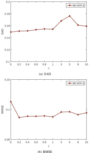
1) Parameter setting: The matrix-vector NTF based unmix-ing method has two forms: one without sum-to-one constraint and the other with this constraint. For simplicity, we abbreviate them as MV-NTF and MV-NTF-S respectively. Here we will compare MV-NTF and MV-NTF-S on synthetic data to see the effect of sum-to-one constraint. Therefore, we first present in Fig. 3 the result of MV-NTF-S on clean synthetic data (z= 8
and θ = 0.7) with respect to the parameter δ that controls the impact of sum-to-one constraint on the cost function in
0 50 100 150 200 Band 0 0.1 0.2 0.3 0.4 0.5 0.6 0.7 0.8 0.9 1 Reflectance Carnallite NMNH98011 Ammonio-jarosite SCR-NHJ Almandine WS478 Brucite HS247.3B Axinite HS342.3B Chlorite HS179.3B
Fig. 2. The spectral signatures of six endmembers used in synthetic data.
Equation 35. It should be noted that MV-NTF-S with δ = 0
equals to MV-NTF without sum-to-one constraint. From Fig. 3, we can see that when δ <1, SAD has very little change, and RMSE is stable when 0.2 < δ < 1. In the following experiment, we set δ= 0.4for MV-NTF-S.
0 0.2 0.4 0.6 0.8 1 3 5 8 10 δ 0.1 0.12 0.14 0.16 0.18 0.2 SAD MV-NTF-S (a) SAD 0 0.2 0.4 0.6 0.8 1 3 5 8 10 δ 0.05 0.1 0.15 RMSE MV-NTF-S (b) RMSE
Fig. 3. SAD and RMSE with respect to the impact of sum-to-one constraint.
For matrix-vector NTF based unmixing algorithm, the num-ber of endmemnum-bers R and the rank of abundance matrix Lr
are two important model parameters. In practice, the number
of endmembers can be obtained by the domain knowledge or other estimation methods, so here we only discuss the impact ofLr on the unmixing performance. A lot of studies
have demonstrated that the distribution of abundances in an HSI is always low rank, so Lr is a good index to reflect
the distribution of abundance. Here we evaluate the unmixing performance with respect to rank changes. For simplicity, we let Lr = L for r = 1,2, . . . , R, which can greatly reduce
the complexity of model. In the experiment, we set z = 8,
SN R= 30andθ= 0.7 for the synthetic data.
Fig. 4 shows the unmixing results with different ranks of abundance matrix, from which we find that both SAD and RMSE do not simply decrease or increase with the rank changes, but have little oscillations. However, in a large range of 20 ≤ L ≤ 60, the unmixing performance is basically stable on a high level (some oscillations might be caused by initialization of optimization and noise disturbance), which implies that the determination of the parameter L is not a difficult problem for the matrix-vector NTF based unmixing algorithm. The spatial size of the synthetic HSI is 64×64, i.e., the maximal rank of the abundance matrix is 64. The experimental results give us a simple guidance on choosing the value of rank: except for very large or very small ranks, all other values can be accepted. Compared with other sparsity or low rank based unmixing algorithms, the parameter setting of our method is much easier in real applications. In the following experiments, we setL≈2
3min(I, J).
2) Method comparison under different noise levels: In this experiment, we compare the unmixing performance of four methods NMF, L1/2-NMF, MRS-NMF, NTF and
MV-NTF-S under different noise levels. Adding Gaussian noise into clean HSI might cause some pixels to have negative values in their spectral signatures, especially the noise level is high. In this case, these negative values are simply reset to zero.
The parametersz= 8andθ= 0.7are set for all noisy data. In order to ensure fair comparison, we first randomly initialize Ar,BTr, r = 1, . . . R for matrix-vector NTF, and then use
ArBTr as the initialized abundance maps of NMF,L1/2-NMF, and MRS-NMF. At the same time, all five methods have the same randomly initialized endmembers. The comparison results are shown in Tables I and II, and Fig. 5, from which it can be found that matrix-vector NTF is much better than other algorithms under different noise levels. As expected, NMF delivers the worst results in terms of both SAD and RMSE because it does not have a sparsity regularizer and misses spectral-spatial structure. L1/2-NMF and MRS-NMF have very similar SAD results, but MRS-NMF has less RMSE than L1/2-NMF, which shows the spectral-spatial informa-tion embedded in MRS-NMF is beneficial to the abundance estimation of a whole image. Meanwhile, their L1/2 norm based sparsity constraint is very helpful to both endmember and abundance estimation. Our matrix-vector NTF not only preserves the intrinsic spectral-spatial joint structure of an HSI, but also allows low-rank representation for abundance maps, which makes it more effective than other unmixing methods such asL1/2-NMF and MRS-NMF that externally enforce the
constraints of spectral-spatial structure and sparsity into NMF model. In general, the performance of all unmixing methods
5 15 25 35 45 55 Rank 0.1 0.15 0.2 0.25 0.3 SAD MV-NTF MV-NTF-S (a) SAD 5 15 25 35 45 55 Rank 0.05 0.1 0.15 0.2 RMSE MV-NTF MV-NTF-S (b) RMSE
Fig. 4. SAD and RMSE with respect to the rank of abundance matrix. TABLE I
SADOF THE UNMIXING METHODS WITH RESPECT TO THE NOISE LEVEL.
SNR 15 20 25 30 35 Inf NMF 0.3373 0.3275 0.3189 0.2738 0.2736 0.2734 L1/2-NMF 0.2187 0.2022 0.2015 0.1813 0.1806 0.1816 MRS-NMF 0.2152 0.2020 0.2016 0.1807 0.1795 0.1794 MV-NTF 0.1747 0.1732 0.1689 0.1520 0.1525 0.1512 MV-NTF-S 0.1757 0.1700 0.1648 0.1519 0.1526 0.1512 TABLE II
RMSEOF THE UNMIXING METHODS WITH RESPECT TO THE NOISE LEVEL.
SNR 15 20 25 30 35 Inf NMF 0.1509 0.1485 0.1486 0.1481 0.1480 0.1480 L1/2-NMF 0.1450 0.1393 0.1367 0.1357 0.1349 0.1348 MRS-NMF 0.1435 0.1371 0.1357 0.1346 0.1328 0.1231 MV-NTF 0.1018 0.1021 0.1026 0.0972 0.1012 0.1035 MV-NTF-S 0.0925 0.0901 0.0906 0.0868 0.0865 0.0887
is becoming worse as the noise level increases, but both of MV-NTF and MV-NTF-S are more robust to the noise than other methods.
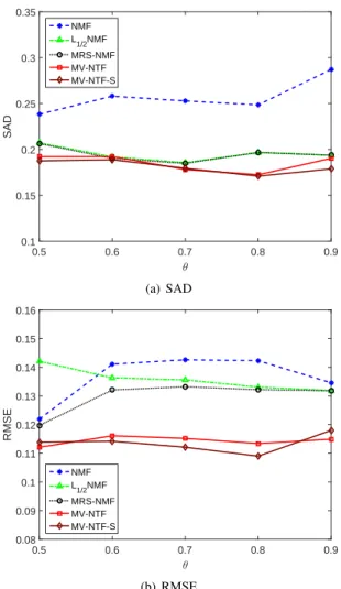
3) Method comparison under different mixing levels: This experiment aims at evaluating the performance of five unmix-ing algorithms in the synthetic HSI data with different mixunmix-ing levels. The mixing level is controlled by the parameter θ in data generation, i.e., a largerθimplies smaller mixing level. In
∞ 35 30 25 20 15 SNR(dB) 0.1 0.15 0.2 0.25 0.3 0.35 0.4 SAD NMF L1/2NMF MRS-NMF MV-NTF MV-NTF-S (a) SAD ∞ 35 30 25 20 15 SNR(dB) 0.06 0.08 0.1 0.12 0.14 0.16 0.18 0.2 0.22 RMSE NMF L1/2NMF MRS-NMF MV-NTF MV-NTF-S (b) RMSE
Fig. 5. SAD and RMSE with respect to the noise level. TABLE III
SADOF THE UNMIXING METHODS UNDER DIFFERENT MIXING LEVELS.
θ 0.5 0.6 0.7 0.8 0.9 NMF 0.2383 0.2580 0.2528 0.2485 0.2871 L1/2-NMF 0.2071 0.1920 0.1855 0.1967 0.1936 MRS-NMF 0.2064 0.1902 0.1848 0.1967 0.1937 MV-NTF 0.1921 0.1922 0.1781 0.1724 0.1903 MV-NTF-S 0.1875 0.1887 0.1794 0.1709 0.1788 TABLE IV
RMSEOF THE UNMIXING METHODS UNDER DIFFERENT MIXING LEVELS.
θ 0.5 0.6 0.7 0.8 0.9 NMF 0.1219 0.1411 0.1426 0.1423 0.1346 L1/2-NMF 0.1421 0.1363 0.1356 0.1331 0.1319 MRS-NMF 0.1197 0.1321 0.1332 0.1322 0.1318 MV-NTF 0.1121 0.1161 0.1152 0.1134 0.1149 MV-NTF-S 0.1139 0.1142 0.1121 0.1090 0.1180
the experiment, we setz= 8andSN R= 25for all synthetic HSI data. The SAD and RMSE of five unmixing methods in the synthetic HSI data with θ = 0.5,0.6,0.7,0.8,0.9
respectively are shown in Tables III, IV and Fig. 6. We found that both of MV-NTF and MV-NTF-S are better than other three methods in terms of SAD and RMSE. Generally, all five methods under comparison are not sensitive to the mixing level.
0.5 0.6 0.7 0.8 0.9 θ 0.1 0.15 0.2 0.25 0.3 0.35 SAD NMF L1/2NMF MRS-NMF MV-NTF MV-NTF-S (a) SAD 0.5 0.6 0.7 0.8 0.9 θ 0.08 0.09 0.1 0.11 0.12 0.13 0.14 0.15 0.16 RMSE NMF L 1/2NMF MRS-NMF MV-NTF MV-NTF-S (b) RMSE
Fig. 6. SAD and RMSE with respect to the mixing level. TABLE V
SADOF THE UNMIXING METHOD UNDER DIFFERENT IMAGE SIZES. Sample Size 1296 2401 4096 6561 10000 NMF 0.3515 0.2619 0.2528 0.2614 0.2693 L1/2-NMF 0.2567 0.2479 0.1855 0.1994 0.1771 MRS-NMF 0.2592 0.2509 0.1848 0.1997 0.1741 MV-NTF 0.2256 0.2091 0.1781 0.1720 0.1503 MV-NTF-S 0.2021 0.2008 0.1794 0.1716 0.1355
4) Method comparison under different image sizes: This experiment is used for evaluating five unmixing methods in the synthetic data with different sizes of image (number of pixels in an HSI). The sizes of image are chosen as36×36,
49×49,64×64,81×81, and100×100respectively. The other parameters are set as SN R= 25 andθ= 0.7. Tables V, VI and Fig. 7 show the unmixing performance of all methods in terms of SAD and RMSE. It can be seen that their performance becomes to be better as the image size increases, which demonstrates that the spectral, spatial, and their joint structures of an HSI is very helpful to solve the unmixing problem. Large image size implies the richness of the structural information within it. Under all image sizes, MV-NTF and MV-NTF-S are better than the other three approaches.
After comparing the above experiments results, it can be found that MV-NTF and MV-NTF-S are very similar and both of them are better than NMF, L1/2-NMF and MRS-NMF.
TABLE VI
RMSEOF THE UNMIXING METHODS UNDER DIFFERENT IMAGE SIZES. Sample Size 1296 2401 4096 6561 10000 NMF 0.1573 0.1447 0.1426 0.1434 0.1259 L1/2-NMF 0.1556 0.1388 0.1356 0.1375 0.1133 MRS-NMF 0.1536 0.1368 0.1332 0.1353 0.1077 MV-NTF 0.1260 0.1047 0.1152 0.0805 0.0900 MV-NTF-S 0.1189 0.1093 0.1121 0.1020 0.0968 1296 2401 4096 6561 10000 Number of pixels 0.1 0.15 0.2 0.25 0.3 0.35 0.4 SAD NMF L1/2NMF MRS-NMF MV-NTF MV-NTF-S (a) SAD 1296 2401 4096 6561 10000 Number of pixels 0.05 0.1 0.15 0.2 RMSE NMF L 1/2NMF MRS-NMF MV-NTF MV-NTF-S (b) RMSE
Fig. 7. SAD and RMSE with respect to the image size. B. Experiments on real-world Data
Three real-world data sets were used to evaluate the pro-posed matrix-vector NTF method: Urban, Jasper, and Cuprite. These three HSI data have different numbers of endmembers, sizes of image, and acquisition sensors, which help us compre-hensively evaluate the unmixing performance. Four unmixing methods NMF, L1/2-NMF, MRS-NMF, and VCA-FCLS [5] were chosen for comparison. The parameter settings of these algorithm were according to their original papers. As the unmixing performance of MV-NTF-S is slightly better than MV-NTF on synthetic data, we use matrix-vector NTF with sum-to-one constraint algorithm for real-world data.
1) HYDICE Urban Data set: This data set was generated by the Hyperspectral Digital Imagery Collection Experiment (HYDICE) on an urban area. Its size is307×307and it has 210 spectral channels with spectral resolution of 10nm acquired in the 400nm and 2500nm range. After low SNR bands had
Fig. 8. The 80th band image of HYDICE Urban data set.
been removed, 162 bands remained for the experiments. Fig. 8 shows its 80th band image. We set the number of endmembers as 4, including roof, grass, asphalt and tree.
In order to give quantitative evaluation results, we use the method in [16], [17] to obtain the reference endmembers and abundances of HYDICE Urban data set. The reference endmember spectra of various materials are manually chosen from the hyperspectral data itself, e.g., the spectrum in the coordinate position of (78,220)in HYDICE Urban image is selected as the asphalt spectrum, which is very similar to the asphalt spectrum in the spectral library. Once the reference endmembers are determined, their corresponding reference abundances are computed by the method of least squares, subject to sum-to-one and positivity constraints [7].
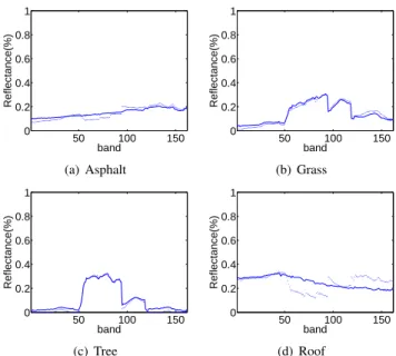
The SAD results of the unmixing methods are shown in Table VII. It can be seen that matrix-vector NTF is better than the other four methods. Fig. 9 shows the estimated endmember signatures of matrix-vector NTF against references. We found that the estimated endmember signatures are very close to their corresponding reference ones. Fig. 10 shows the reference abundance maps and estimated abundance maps respectively. All these results demonstrate that the proposed matrix-vector NTF can achieve a competitive unmixing performance com-pared with the state-of-the-art unmixing approaches on this data set.
2) Jasper Ridge Data set: Jasper Ridge data set was col-lected by the Airborne Visible/Infrared Imaging Spectrometer (AVIRIS) over Jasper Ridge in central California, USA. It contains 224 bands covering the wavelengths from 0.38µm to 2.5µm, with a 10 nm spectral resolution. The size of original image is512×614. We only used a part of it with the size of
100×100, whose 80th band image is shown in Fig. 11. We removed some low SNR and water-vapor absorption bands so that 198 bands were retained. Four endmembers are assumed in the image, which are soil, water, tree and road. Its reference endmembers and abundances are obtained by the same method used for HYDICE Urban data.
The comparative SAD results of five methods are given in Table VIII. Matrix-vector NTF and MRS-NMF are better than other methods. Matrix-vector NTF outperforms MRS-NMF in terms of the mean SAD of all four endmembers. The estimated endmember signatures of matrix-vector NTF against the references are shown in Fig. 12, from which we
50 100 150 0 0.2 0.4 0.6 0.8 1 band Reflectance(%) (a) Asphalt 50 100 150 0 0.2 0.4 0.6 0.8 1 band Reflectance(%) (b) Grass 50 100 150 0 0.2 0.4 0.6 0.8 1 band Reflectance(%) (c) Tree 50 100 150 0 0.2 0.4 0.6 0.8 1 band Reflectance(%) (d) Roof
Fig. 9. Endmembers of HYDICE Urban estimated by matrix-vector NTF. Solid lines denote the reference endmembers and dashed lines denote the estimated endmembers.
Fig. 11. The 80th band image of Jasper Ridge data set.
can see that their difference is very small. All abundance maps generated by five algorithms are shown in Fig. 13.
3) Cuprite Data set: The third real HSI was acquired by AVIRIS over Cuprite in southern Nevada, USA. As the minerals are highly mixed in the scene and the number of main materials is up to 10, this data has been widely used to investigate the performance of various unmixing algorithms. The cuprite data contains 224 bands with the wavelength from
0.4µm to2.5µm. In the experiments, a region with the size of
250×191selected from the original data set was used. Fig. 14 shows the 80th band image of this data set. After removing the low SNR and water vapor absorption bands, 188 bands remained for the experiments.
For Cuprite data set, the reference endmembers and abun-dances about this scene have been reported in [54] which used the spectral correlation between a scaled laboratory reference spectrum and ground calibrated Cuprite data for each pixel, and the library spectrum with the highest correlation is chosen as the best match. The library spectra of the main minerals in the scene are selected as the ground truth of endmembers, and the quality of fit for each mineral is calculated for each pixel and the results are considered as the reference abundances.
TABLE VII
MEANS AND STANDARD DEVIATIONS OF SAD ON HYDICE URBANDATA.
Algorithm NMF L1/2-NMF MRS-NMF VCA-FCLS MV-NTF Asphal 0.1347±4.05% 0.1089±0.74% 0.1223±1.21% 0.4307±44.08% 0.1638±0.87% Grass 0.8479±45.40% 0.1604±4.67% 0.1716±7.93% 0.41.33±0.00% 0.2268±13.64% Tree 0.1331±0.68% 0.2869±6.83% 0.2229±12.20% 0.3083±6.57% 0.1054±3.26% Roof 0.9176±13.21% 0.4438±13.33% 0.4346±15.59% 0.7443±14.89% 0.3707±2.33% Mean 0.5083±13.50% 0.2500±5.04% 0.2378±6.62% 0.4742±7.67% 0.2167±2.25%
(a) MV-NTF (b) NMF (c)L1/2-NMF (d) MRS-NMF (e) VCA-FCLS (f) Reference
Fig. 10. Estimated abundance maps by five unmixing algorithms on the HYDICE Urban data set. From top to bottom, the rows are the abundance maps of asphalt, grass, tree, roof.
TABLE VIII
MEANS AND STANDARD DEVIATIONS OF SAD ON JASPERRIDGE DATA
Algorithm NMF L1/2-NMF MRS-NMF VCA-FCLS MV-NTF Tree 0.2199±2.91% 0.1142±7.40% 0.0833±6.93% 0.2576±4.58% 0.2126±1.74% Water 0.3372±3.42% 0.1515±0.73% 0.1275±0.57% 0.2517±0.31% 0.2519±0.86% Soil 0.1514±5.25% 0.1111±3.53% 0.0671±1.39% 0.4483±20.76% 0.1504±7.77% Road 1.1626±8.33% 0.7793±2.31% 0.7993±7.98% 0.5371±1.08% 0.2180±14.98% Mean 0.4678±3.64% 0.2891±2.95% 0.2693±2.73% 0.3737±5.09% 0.2082±6.00%
The SAD results of five methods are given in Table IX. It can be found that the mean SAD of the proposed matrix-vector NTF based unmixing method is slightly smaller than the results of other methods. The estimated endmember signatures of matrix-vector NTF and their references are shown in Fig. 15. From the experiments on Cuprite data, we can see that matrix-vector NTF still has a good performance even though this data set is relatively difficult to process due to a large
number of endmembers.
C. Discussion
Through the experiments on the above synthetic and real HSI data sets, the proposed matrix-vector NTF demonstrates competitive unmixing performance against several state-of-the-art NMF based methods. Both matrix-vector NTF and basic NMF have not introduced any constraint on spectral,
(a) MV-NTF (b) NMF (c)L1/2-NMF (d) MRS-NMF (e) VCA-FCLS (f) Reference
Fig. 13. Estimated abundance maps by five unmixing methods on the Jasper Ridge data set. From top to bottom, the rows are the abundance maps of tree, water, soil, and road.
TABLE IX
MEANS AND STANDARD DEVIATIONS OF SAD ON CUPRITE DATA.
Algorithm NMF L1/2-NMF MRS-NMF VCA-FCLS MV-NTF Alunite 0.1408±4.31% 0.1464±5.45% 0.1380±2.68% 0.1109±3.07% 0.1410±3.05% Andradite 0.1341±8.96% 0.0828±2.73% 0.0805±2.40% 0.0684±1.22% 0.1120±6.87% Buddingtonite 0.1656±0.67% 0.1507±0.95% 0.1495±0.81% 0.0752±5.52% 0.0835±0.26% Dumortierite 13.96±1.32% 0.1175±2.56% 0.1219±2.25% 0.1722±2.89% 0.1514±1.35% Kaolinite 0.1990±6.04% 0.1962±4.65% 0.0561±0.27% 0.2139±1.81% 0.0932±2.26% Montmorillonite 0.1002±0.34% 0.0943±1.40% 0.1526±7.58% 0.1770±1.47% 0.1633±2.65% Muscovite 0.1416±0.08% 0.1456±0.87% 0.1110±2.53% 0.2044±2.61% 0.1376±1.13% Nontronite 0.0818±0.34% 0.1154±3.94% 0.1490±8.68% 0.0670±2.87% 0.0793±0.18% Pyrope 0.0631±1.87% 0.0731±0.41% 0.0729±0.43% 0.0963±6.58% 0.0547±0.55% Sphene 0.0594±1% 0.0962±0.52% 0.1063±1.90% 0.0703±6.08% 0.1017±3.29 % Mean 0.1225±0.63% 0.1218±1.16% 0.1138±1.30% 0.1255±0.38% 0.1118±1.24%
spatial, or spectral-spatial structures of an HSI, while other two NMF based methods use abundance sparsity and spectral-spatial manifold information as constraints. The experimental results confirm that the matrix-vector NTF can preserve the HSI structure as it treats an HSI cube as a whole processing frame. It overcomes the drawback of NMF based unmixing models that the structural information is lost when unfolding an HSI cube into a matrix. L1/2-NMF and MRS-NMF as typical constrained NMF based unmixing methods aim to embed the spatial and spectral structures of an HSI into NMF model, and have been proved to generate more reasonable unmixing results. Different from their external and explicit
method, matrix-vector NTF achieves this aim by the intrinsic structure and the operations of tensor decomposition, which is more interpretable and easier to complete. Furthermore, its performance is somehow better than these two approaches. In summary, our proposed method provides an alternative and effective technique for blind spectral unmixing.
V. CONCLUSION
In this paper, a new tensor decomposition based unmixing method, matrix-vector NTF, is proposed. Tensor is a more natural and accurate representation method for HSI cube than matrix. However, building a link between tensor decompo-sition and linear spectral mixture model is not an easy task.
50 100 150 0 0.2 0.4 0.6 0.8 1 band Reflectance(%) (a) Tree 50 100 150 0 0.2 0.4 0.6 0.8 1 band Reflectance(%) (b) Water 50 100 150 0 0.2 0.4 0.6 0.8 1 band Reflectance(%) (c) Soil 50 100 150 0 0.2 0.4 0.6 0.8 1 band Reflectance(%) (d) Road
Fig. 12. Endmembers of Jasper Ridge estimated by matrix-vector NTF. Solid lines denote the reference endmembers and dashed lines denote the estimated endmembers.
Fig. 14. Cuprite hyperspectral dataset at band 80.
We firstly introduce two popular tensor decomposition models, CPD and Tucker decomposition, analyze their relationship with linear spectral mixture model, and point out their lack of straightforward link with linear spectral mixture model in the view of physical and mathematical mechanisms. After that, the matrix-vector tensor decomposition as a special BTD is proposed for unmixing, which is fully consistent to the linear spectral mixture model under tensor notation, leading to clear physical and mathematical interpretation and easy implementation. In order to satisfy the nonnegative property of endmember and abundance, matrix-vector NTF is presented, and its alternating least square optimization algorithm is derived. Moreover, the uniqueness of matrix-vector NTF and the convergence of optimization algorithm are also discussed. The experiments on synthetic and real data sets demonstrated the advantages of our unmixing method against a number of alternatives, i.e., NMF,L1/2-NMF, and MRS-NMF. The main
object of this paper is to extend NMF based unmixing method to tensor frame, so we just give a basic matrix-vector NTF
50 100 150 0 0.2 0.4 0.6 0.8 1 band Reflectance(%) (a) Alunite 50 100 150 0 0.2 0.4 0.6 0.8 1 band Reflectance(%) (b) Andradite 50 100 150 0 0.2 0.4 0.6 0.8 1 band Reflectance(%) (c) Buddingtonite 50 100 150 0 0.2 0.4 0.6 0.8 1 band Reflectance(%) (d) Dumortierite 50 100 150 0 0.2 0.4 0.6 0.8 1 band Reflectance(%) (e) Kaolinite 50 100 150 0 0.2 0.4 0.6 0.8 1 band Reflectance(%) (f) Montmorillonite 50 100 150 0 0.2 0.4 0.6 0.8 1 band Reflectance(%) (g) Muscovite 50 100 150 0 0.2 0.4 0.6 0.8 1 band Reflectance(%) (h) Nontronite 50 100 150 0 0.2 0.4 0.6 0.8 1 band Reflectance(%) (i) Pyrope 50 100 150 0 0.2 0.4 0.6 0.8 1 band Reflectance(%) (j) Sphene
Fig. 15. Endmembers of Cuprite estimated by matrix-vector NTF. Solid lines denote the reference endmembers and dashed lines denote the estimated endmembers.
model. It should be emphasised that like NMF based unmixing model, the proposed NTF model is quite general in nature, so it can incorporate other information or constraints such as sparsity, nonlinear mixture, local consistence, and insensitive-ness to noise. New unmixing models and approaches can be developed based on it.
REFERENCES
[1] J. Bioucas-Dias, A. Plaza, N. Dobigeon, M. Parente, Q. Du, P. Gader, and J. Chanussot, “Hyperspectral unmixing overview: Geometrical, statistical, and sparse regression-based approaches,” IEEE J. Select. Topics Appl. Earth Observ. Remote Sens., vol. 5, no. 2, pp. 354–379, 2012.
[2] W. Ma, J. Bioucas-Dias, T. Chan, and et al., “A signal processing perspective on hyperspectral unmixing: Insights from remote sensing signal processing magazine,”IEEE Signal Process. Mag., vol. 31, no. 1, pp. 67–81, 2014.
[3] J. Boardman, “Automating spectral unmixing of AVIRIS data using convegeometry concepts,” inProc. AVIRIS Workshop, vol. 1, 1993, pp. 11–14.
[4] M. E. Winter, “N-FINDR: an algorithm for fast autonomous spectral end-member determination in hyperspectral data,” inProc. SPIE Conf. Imag. Spectr. V, vol. 3753, 1999, pp. 266–275.
[5] J. Nascimento and J. Bioucas-Dias, “Vertex component analysis: a fast algorithm to unmix hyperspectral data,”IEEE Trans. Geosci. Remote Sens., vol. 43, no. 4, pp. 898–910, 2005.
[6] J. Li, A. Agathos, D. Zaharie, J. Bioucas-Dias, A. Plaza, and X. Li, “Minimum volume simplex analysis: A fast algorithm for linear hyper-spectral unmixing,”IEEE Trans. Geosci. Remote Sens., vol. 53, no. 9, pp. 5067–5082, 2015.
[7] D. Heinz and C.-I. Chang, “Fully constrained least squares linear spectral mixture analysis method for material quantification in hyperspectral imagery,”IEEE Trans. Geosci. Remote Sens., vol. 39, no. 3, pp. 529– 545, 2001.
[8] M. Iordache, J. Bioucas-Dias, and A. Plaza, “Sparse unmixing of hyperspectral data. geoscience and remote sensing,”IEEE Trans. Geosci. Remote Sens., vol. 49, no. 6, pp. 2014–2039, 2011.
[9] F. Schmidt, A. Schmidt, E. Treguier, M. Guiheneuf, S. Moussaoui, and N. Dobigeon, “Implememtation strategies for hyperspectral unmixng using bayesian source separation,”IEEE Trans. Geosci. Remote Sens., vol. 48, no. 11, pp. 4003–4013, 2010.
[10] S. Jia and Y. Qian, “Spectral and spatial complexity-based hyperspectral unmixing,”IEEE Trans. Geosci. Remote Sens., vol. 45, no. 12, pp. 3867– 3879, 2007.
[11] L. Tong, J. Zhou, Y. Qian, X. Bai, and Y. Gao, “Nonnegative matrix factorization based hyperspectral unmixing with partially known end-members,”IEEE Trans. Geosci. Remote Sens., vol. 54, no. 11, pp. 6531– 6544, 2016.
[12] L. Miao and H. Qi, “Endmember extraction from highly mixed data using minimum volume constrained nonnegative matrix factorization,”
IEEE Trans. Geosci. Remote Sens., vol. 45, no. 3, pp. 765–777, 2007. [13] S. Jia and Y. Qian, “Constrained nonnegative matrix factorization for
hyperspectral unmixing,”IEEE Trans. Geosci. Remote Sens., vol. 47, no. 1, pp. 161–173, 2009.
[14] A. Cichocki, R. Zdunek, A. H. Phan, and S. Amari,Nonnegative Matrix and Tensor Factorizations: applications to exploratory multi-way data analysis and blind source separation. Wiley, 2009.
[15] D. Thompson, R. Castao, and M. Gilmore, “Sparse superpixel unmixing for exploratory analysis of CRISM hyperspectral images,” inProc. of the IEEE Workshop on Hyperspectral Image and Signal Processing: Evolution in Remote Sensing, 2009, pp. 1–4.
[16] Y. Qian, S. Jia, J. Zhou, and A. Robles-Kelly, “Hyperspectral unmixing viaL1/2 sparsity-constrained nonnegative matrix factorization,”IEEE
Trans. Geosci. Remote Sens., vol. 49, no. 11, pp. 4282–4297, 2011. [17] W. Wang and Y. Qian, “AdaptiveL1/2sparsity-constrained NMF with
half-thresholding algorithm for hyperspectral unmixing,”IEEE J. Select. Topics Appl. Earth Observ. Remote Sens., vol. 8, no. 6, pp. 2618–2631, 2015.
[18] X. Liu, W. Xia, B. Wang, and L. Zhang, “An approach based on constrained nonnegative matrix factorization to unmix hyperspectral data,”IEEE Trans. Geosci. Remote Sens., vol. 49, no. 2, pp. 757–772, 2011.
[19] S. Mei, M. He, Z. Shen, and B. Belkacem, “Neighborhood preserving nonnegative matrix factorization for spectral mixture analysis,” inProc. IEEE IGARSS, 2013, pp. 2573–2576.
[20] X. Lu, H. Wu, Y. Yuan, P. Yan, and X. Li, “Manifold regularized sparse NMF for hyperspectral unmixng,”IEEE Trans. Geosci. Remote Sens., vol. 51, no. 5, pp. 2815–2826, 2013.
[21] W. Wang, Y. Qian, J. Zhou, and Y. Y. Tang, “Hypergraph-regularized sparse nmf for hyperspectral unmixing,”IEEE J. Select. Topics Appl. Earth Observ. Remote Sens., vol. 9, no. 2, pp. 681–694, 2016. [22] T. Kolda and B. Bader, “Tensor decompositions and applications,”SIAM
review, vol. 51, no. 3, pp. 455–500, 2009.
[23] T. Hazan, S. Polak, and A. Shashua, “Sparse image coding using a 3d non-negative tensor factorization,” inIEEE International Conference on Computer Vision (ICCV2005), 2005, pp. 50–57.
[24] S. Khan and S. Kaski, “Bayesian multi-view tensor factorization,” in
Machine Learning and Knowledge Discovery in Databases, Springer Berlin Heidelberg, 2014, pp. 656–671.
[25] A. Cichocki, D. Mandic, L. De Lathauwer, G. Zhou, Q. Zhao, C. Caiafa, and H. Phan, “Tensor decompositions for signal processing applications: From two-way to multiway component analysis,”IEEE Signal Process-ing Magazine, vol. 32, no. 2, pp. 145–163, 2015.
[26] U. Schaechtle, K. Stathis, and S. Bromuri, “Multi-dimensional causal discovery,” inInternational Joint Conference on Artificial Intelligence (IJCAI), 2013.
[27] A. Karami, M. Yazdi, and G. Mercier, “Compression of hyperspectral images using discerete wavelet transform and tucker decomposition,”
IEEE J. Select. Topics Appl. Earth Observ. Remote Sens., vol. 5, no. 2, pp. 444–450, 2012.
[28] L. Zhang, L. Zhang, D. Tao, X. Huang, and B. Du, “Compression of hyperspectral remote sensing images by tensor approach,” Neurocom-puting, vol. 147, pp. 358–363, 2015.
[29] D. Liao, M. Ye, S. Jia, and Y. Qian, “Noise reduction of hyperspectral imagery based on nonlocal tensor factorization,” inIEEE International Geoscience and Remote Sensing Symposium, 2013.
[30] X. Guo, X. Huang, L. Zhang, and L. Zhang, “Hyperspectral image noise reduction based on rank-1 tensor decomposition,”ISPRS Journal of Photogrammetry and Remote Sensing, vol. 83, pp. 50–63, 2013. [31] C. Li, Y. Ma, J. Huang, X. Mei, and J. Ma, “Hyperspectral image
denoising using the robust low-rank tensor recovery. josa a, 32(9), 1604-1612.”Journal of the Optical Society of America A, vol. 32, no. 9, pp. 1604–1612, 2015.
[32] L. Zhang, L. Zhang, D. Tao, and X. Huang, “Tensor discriminative local-ity alignment for hyperspectral image spectralcspatial feature extraction,”
IEEE Trans. Geosci. Remote Sens., vol. 51, no. 1, pp. 242–256, 2013. [33] Z. Chen, B. Wang, Y. Niu, W. Xia, J. Zhang, and B. Hu, “Change
detection for hyperspectral images based on tensor analysis,” in IEEE International Geoscience and Remote Sensing Symposium, 2015. [34] S. Li, W. Wang, H. Qi, B. Ayhan, C. Kwan, and S. Vance,
“Low-rank tensor decomposition based anomaly detection for hyperspectral imagery,” inIEEE International Conference on Image Processing (ICIP), 2015, pp. 4525–4529.
[35] S. Bourennane, C. Fossati, and A. Cailly, “Improvement of classification for hyperspectral images based on tensor modeling,” IEEE Geosci. Remote Sens. Lett., vol. 7, no. 4, pp. 801–805, 2010.
[36] X. Guo, X. Huang, L. Zhang, L. Zhang, A. Plaza, and A. Benediktsson, “Support tensor machines for classification of hyperspectral remote sensing imagery,” IEEE Trans. Geosci. Remote Sens., vol. 54, no. 6, pp. 3248–3264, 2016.
[37] Q. Zhang, H. Wang, R. Plemmons, and V. Pauca, “Spectral unmixing using nonnegative tensor factorization,” in Proc. ACM 45th annual southeast regional conference, 2007, pp. 531–532.
[38] ——, “Tensor methods for hyperspectral data analysis: a space object material identification study,”Journal of the Optical Society of America A, vol. 25, no. 12, pp. 3001–3012, 2008.
[39] A. Huck and M. Guillaume, “Estimation of the hyperspectral tucker ranks.” in IEEE International Conference on Acoustics, Speech and Signal Processing (ICASSP), 2009, pp. 1281–1284.
[40] M. Veganzones, J. Cohen, R. Farias, R. Marrero, J. Chanussot, and P. Comon, “Multilinear spectral unmixing of hyperspectral multiangle images,” in IEEE European Internationa Conference on European (EUSIPCO), 2015, pp. 4525–4529.
[41] M. Veganzones, J. Cohen, R. Farias, J. Chanussot, and P. Comon, “Nonnegative tensor cp decomposition of hyperspectral data,” IEEE Trans. Geosci. Remote Sens., vol. 54, no. 5, pp. 2577–2588, 2016. [42] R. Heylen and P. Scheunders, “A multilinear mixing model for nonlinear
spectral unmixing,”IEEE Trans. Geosci. Remote Sens., vol. 54, no. 1, pp. 240–251, 2016.
[43] L. De Lathauwer and D. Nion, “Decompositions of a higher-order tensor in block terms-part I: lemma for partitioned matrices,”SIAM Journal on Matrix Analysis and Applications, vol. 30, no. 3, pp. 1022–1032, 2008. [44] G. Favier and A. de Almeida, “Overview of constrained parafac models,”
EURASIP Journal on Advances in Signal Processing, vol. 2014(1), pp. 1–25, 2014.
[45] L. De Lathauwer, “Block component analysis, a new concept for blind source separation,” in International Conference on Latent Variable Analysis and Signal Separation, 2012, pp. 1–8.