Hierarchical Topical Segmentation with Affinity Propagation
Anna Kazantseva & Stan Szpakowicz
School of Electrical Engineering and Computer Science University of Ottawa
Ottawa, Ontario, Canada
{ankazant,szpak}@eecs.uottawa.ca
Abstract
We present a hierarchical topical segmenter for free text. Hierarchical Affinity Propagation for Segmentation (HAPS) is derived from a clustering algorithm Affinity Propagation. Given a doc-ument,HAPSbuilds a topical tree. The nodes at the top level correspond to the most prominent shifts of topic in the document. Nodes at lower levels correspond to finer topical fluctuations. For each segment in the tree,HAPSidentifies a segment centre – a sentence or a paragraph which best describes its contents. We evaluate the segmenter on a subset of a novel manually segmented by several annotators, and on a dataset of Wikipedia articles. The results suggest that hierarchical segmentations produced byHAPSare better than those obtained by iteratively running several one-level segmenters. An additional advantage of HAPS is that it does not require the “gold standard” number of segments in advance.
1 Introduction
When an NLP application works with a document, it may benefit from knowing something about this document’s high-level structure. Text summarization (Haghighi and Vanderwende, 2009), question an-swering (Oh et al., 2007) and information retrieval (Ponte and Croft, 1998) are some of the examples of such applications. Topical segmentation is a lightweight form of such structural analysis: given a sequence of sentences or paragraphs, split it into a sequence oftopical segments, each characterized by a certain degree of topical unity. This is particularly useful for texts with little structure imposed by the author, such as speech transcripts, meeting notes or literature.
The past decade has witnessed significant progress in the area of text segmentation. Most of the topical segmenters (Malioutov and Barzilay, 2006; Eisenstein and Barzilay, 2008; Kazantseva and Szpakowicz, 2011; Misra et al., 2011; Du et al., 2013) can only produce single-level segmentation, a worthy endeavour in and of itself. Yet, to view the structure of a document linearly, as a sequence of segments, is in certain discord with most theories of discourse structure, where it is more customary to consider documents as trees (Mann and Thompson, 1988; Marcu, 2000; Hernault et al., 2010; Feng and Hirst, 2012) or graphs (Wolf and Gibson, 2006). Regardless of the theory, we hypothesize that it may be useful to have an idea about fluctuations of topic in documents beyond the coarsest level. It is the contribution of this work that we develop such a hierarchical segmenter, implement it and do our best to evaluate it.
The segmenter described here is HAPS – Hierarchical Affinity Propagation for Segmentation. It is closely based on a graphical model for hierarchical clustering calledHierarchical Affinity Propagation (Givoni et al., 2011). It is a similarity-based segmenter. It takes as input a matrix of similarities between atomic units of text in the sequence to be segmented (sentences or paragraphs), the desired number of levels in the topical tree and a preference value for each data point and each level. This value captures a prioribelief about how likely it is that this data point is a segment centre at that level. The preference values also control the granularity of segmentation: how many segments are to be identified at each level. The output is a topical tree. For each segment at every level,HAPSalso finds a segment centre, a data point which best describes the segment.
This work is licensed under a Creative Commons Attribution 4.0 International Licence. Page numbers and proceedings footer are added by the organisers. Licence details:http://creativecommons.org/licenses/by/4.0/
The objective function maximized by the segmenter is net similarity – the sum of similarities between all segment centres and their children for all levels of the tree. This function is similar to the objective function of the well-knownk-meansalgorithm, except that here it is computed hierarchically.
It is not easy to evaluateHAPS. We are not aware of comparable hierarchical segmenters other than that in (Eisenstein, 2009) which, unfortunately, is no longer publicly available. Therefore we compared the trees built by HAPS to the results of running iteratively two state-of-the-art flat segmenters. The results are compared on two datasets. A set of Wikipedia articles was automatically compiled by Carroll (2010). The other set, created to evaluateHAPS, consists of nine chapters from the novelMoonstoneby Wilkie Collins. Each chapter was annotated for hierarchical structure by 3-6 people.
The evaluation is based on two metrics, windowDiff (Pevzner and Hearst, 2002) andevalHDS (Car-roll, 2010). Both metrics are less then ideal. They do not give a complete picture of the quality of topical segmentations, but the preliminary results suggest that running a global model for hierarchical segmentation produces better results then iteratively running flat segmenters. Compared to the baseline segmenters,HAPShas an important practical advantage. It does not require the number of segments as an input; this requirement is customary for most flat segmenters.
We also made a rough attempt to evaluate the quality of the segment centres identified byHAPS. Using 20 chapters from several novels of Jane Austen, we compared the centres identified for each chapter against summaries produces by a recent automatic summarizerCohSum(Smith et al., 2012). The basis of comparison was the ROUGE metric (Lin, 2004). While far from conclusive, the results suggest that segment centres identified byHAPSare rather comparable with the summaries produced by an automatic summarizer.
A Java implementation of HAPS and the corpus of hierarchical segmentations for nine chapters of Moonstoneare publicly available. We consider these to be the main contributions of this research.
2 Related work
Most work on topical text segmentation has been done for single-level segmentation. Contemporary approaches usually rely on the idea that topic shifts can be identified by finding shifts in the vocabulary (Youmans, 1991). We can distinguish between local and global models for topical text segmentation. Local algorithms have a limited view of the document. For example, TextTiling (Hearst, 1997) operates by sliding a window through the input sequence and computing similarity between adjacent units. By identifying “valleys” in similarities, TextTiling identifies topic shifts. More recently, Marathe (2010) used lexical chains and Blei and Moreno (2001) used Hidden Markov Models. Such methods are usually very fast, but can be thrown off by small digressions in the text.
Among global algorithms, we can distinguish generative probabilistic models and similarity-based models. Eisenstein and Barzilay (2008) model a document as a sequence of segments generated by latent topic variables. Misra et al. (2011) and Du et al. (2013) have similar models. Malioutov and Barzilay (2006) and (Kazantseva and Szpakowicz, 2011) use similarity-based representations. Both algorithms take as input a matrix of similarities between sentences of the input document; the former uses graph cuts to find cohesive segments, while the latter modifies a clustering algorithm to perform segmentation. Research on hierarchical segmentation has been more scarce. Yaari (1997) produced hierarchical segmentation by agglomerative clustering. Eisenstein (2009) used a Bayesian model to create topical trees, but the system is regrettably no longer publicly available. Song et al. (2011) develop an algorithm for hierarchical segmentation which iteratively splits a document in two at a place where cohesion links are the weakest. A second pass transforms a deep binary tree into a shallow and broad structure.
Any flat segmenter can certainly be used iteratively to create trees of segments by subdividing each segment, but this may be problematic. Topical segmenters are not perfect, so running them iteratively is likely to compound the error. Most segmenters also require the number of segments as an input. This estimate is feasible for flat segmentation. To know in advance the number of segments and sub-segments at each level is not a realistic requirement when building a tree.
whole tree. It does not need to know the exact number of segments. Instead, it takes a more abstract parameter, preference values, to specify the granularity of segmentation at each level. For each segment it also outputs a segment centre, a unit of text which best captures the contents of the segment.
3 Creating a corpus of hierarchical segmentations
Before embarking on the task of building a hierarchical segmenter, we wanted to study how people perform such a task. We also needed a benchmark corpus which could be used to evaluate the quality of segmentations produced byHAPS.
To this end, we annotated nine chapters of the novelMoonstonefor hierarchical structure. We settled on these data because it is a subset of a publicly available dataset for flat segmentation (Kazantseva and Szpakowicz, 2012). In our study, each chapter was annotated by 3-6 people (4.8on average). The annotators, undergraduate students of English, were paid $50 dollars each.
Procedure. The instructions asked the annotator to read the chapter and split it into top-level segments according to where there is a perceptible shift of topic. She had to provide a one-sentence description of what the segment is about. The procedure had to be repeated for each segment all the way down to the level of individual paragraphs. Effectively, the annotators were building a detailed hierarchical outline for each chapter.
Metrics. Two different metrics helped estimate the quality of our hierarchical dataset: windowDiff (Pevzner and Hearst, 2002) andS(Fournier and Inkpen, 2012).
windowDiff is computed by sliding a window across the input sequence and checking, for each window position, whether the number of reference breaks is the same as the number of breaks in the hypothetical segmentation. The number of erroneous windows is then normalized by the total number of windows. In Equation 1,N is the length of the input sequence andkis the size of the sliding window.
windowDiff = N1−kNX−k
i=1
(|ref −hyp| 6= 0) (1)
windowDiff is designed to compare sequences of segments, not trees. That is why we compute it for each level between each pair of annotators who worked on the same chapter. It should be noted that windowDiffis a penalty metric: higher values indicate less agreement (windowDiff= 0corresponds to two identical segmentations).
TheSmetric allows us to compare trees and take into account situations when the segmenter places a boundary at a correct position but at a wrong level. Sis an edit-distance metric. It computes the number of operations necessary to turn one segmentation into another. There are three types of editing operations: add/delete, transpose and substitute (change the level in the tree). The sum is normalized by the number of possible boundaries in the sequence. S has an unfortunate downside of being too optimistic, but it allows the breakdown of error types and it explicitly compares trees.
UnlikewindowDiff,Sis a similarity metric: higher values correspond to more similar segmentations. The value ofSbetween two identical segmentations is1.
S(bsa, bsb, n) = 1− |boundary distancepb(D) (bsa, bsb, n)| (2)
Hereboundary distance(bsa, bsb, n)is the total number of edit operations needed to turn a
segmen-tation bsa into bsb, nis the threshold defining the maximum distance of transpositions. pb(D) is the
maximum possible number of edits. Segmentations bsa andbsa are represented as strings of sets of
boundary positions. For examplebsa= ({2},{1,2},{1,2}) corresponds to a hierarchical segmentation of
a three-unit sequence in the following manner: a segment boundary at level 1 after the first unit, segment boundaries at levels 1 and 2 after the second unit and the third unit.
in this paper we refer to the bottom level of the tree (i.e., the leaves of the tree or the most fine-grained level of segmentation) as level 1. In Table 1, level 4 refers to the top level of the tree (the coarsest segmentations). The values were computed using only the breaks explicitly specified by the annotators (i.e., we did not assume that a break at a coarse level implies a break at a more detailed level).
The average breadth of the trees at the bottom (level 1) is lower than that at level 2, indicating that only a small percentage of the entire tree was annotated more than three levels deep. The table also shows the average values ofwindowDiff computed for each possible pair of annotators. The values worsen toward the bottom of the tree, suggesting that the annotators agree more about top-level segments and less and less about finer fluctuations of topic.
We hypothesize that these shallow broad structures are due to the fact that it is difficult for people to create deep recursive structures in their mental representations. We do not, however, have any hard data to support this hypothesis. Many of the annotators specifically commented on the difficulty of the task. 9 out of 23 people included comments ranging from notes about specific places to general comments about their lack of confidence. 4 annotators found several (specific) passages they had trouble with.
The average value of pairwiseSis0.79. We have noted earlier that theSmetric tends to be optimistic (that is due to its normalization factor) but it provides a breakdown of disagreements between the anno-tators. According toS,46.14%of disagreements are errors of omission (some of the annotators did not include segment breaks where others did), 47.56%are disagreements about the level of segmentation (the annotators placed boundaries in the same place but at different levels) and only 6.31% are errors of transposition (the annotators do not agree about the exact placement but place boundaries within1 position of each other). This distribution is more interesting than the overall value ofS. Among other things, it shows why it is so important to take into account adjacent levels when evaluating topical trees.
4 TheHAPSalgorithm1
4.1 Factor graphs
The HAPS segmenter is based on factor graphs, a unifying formalism for such graphical models as Markov or Bayesian networks. A factor graph is a bi-partite graph with two types of nodes, factor or function nodesand variable nodes. Each factor node is connected to those variable nodes which are its arguments. Running the well-known Max-Sum algorithm (Bishop, 2006) on a factor graph finds a configuration of variables which maximizes the sum of all component functions. This is a message-passing algorithm. All variable nodes send messages to their factor neighbours (functions in which those nodes are variables) and all factor nodes send messages to their variable neighbours (their arguments). A messageµx→f sent from a variable nodexto a function nodef is computed as a sum of all incoming
messages tox, except the message from the recipient functionf:
µx→f =
X
f0∈N(x)\f
µf0→x (3)
N(x) is the set of all function nodes which arex’s neighbours. Intuitively, the message reflects evi-dence about the distribution ofxfrom all functions which havex as an argument, except the function corresponding to the receiving nodef. A messageµf(x,...)→x sent from the factor nodef(x, ...)to the
1The derivation of theHAPSalgorithm, quite involved, is unlikely to interest many readers. We only present the bare
minimum of facts about the algorithm, the framework of factor graphs and the derivation ofHAPSfrom the underlying model of Affinity Propagation. A detailed account appears in (Kazantseva, 2014).
Table 1: Average breadth of manually created topical trees andwindowDiff value across different levels Level Average breadth windowDiff
4 (top) 6.53 0.35
3 17.55 0.46
2 17.63 0.47
Cl−1
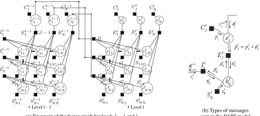
(a) Fragment of the factor graph for levelsl−1andl sent in the(b) Types of messagesHAPSmodel Figure 1: Factor graph forHAPS– Hierarchical Affinity Propagation for Segmentation
variable nodexis computed as a maximum of the value off(x)plus all messages incoming tof(x, ...) other than the message from the recipient nodex:
µf→x = max
N(f)\x(f(x1, . . . , xm) +
X
x0∈N(f)\x
µx0→f) (4)
N(f)is the set of all variable nodes which aref’s neighbours. The message reflects the evidence about the distribution ofxfrom functionf and its neighbours other thanx.
4.2 Hierarchical Affinity Propagation for Segmentation
This work aims to build trees of topical segments. Each segment is characterized by a centre which best describes its content. The objective function is net similarity, the sum of similarities between all centres and the data points which they exemplify. The complete sequence of data points is to be segmented at each level of the tree, subject to the following constraint: centres at each levell,l >1, must be a subset of the centres from the previous levell−1. Figure 1a shows a fragment of the factor graph describing HAPScorresponding to levelslandl−1. The tree hasLlevels, from the root (l=L) down to the leaves (l= 1). The superscripts of factor and variable nodes denote the level.
At each level, there areN2variable nodescl
ijandNvariable nodeselj(N is the number of data points
in the sequence to segment). A variable’s value is 0 or 1:cl
ij = 1⇔the data pointiat levellbelongs to
the segment centred around data pointj;el
j = 1⇔there is a segment centred aroundjat levell.
Four types of factor nodes in Figure 1a areI,E,CandS. TheI factors ensure that each data point is assigned to exactly one segmentandthat segment centres at levellare a subset of those from level
l−1. TheEnodes ensure that segments are centred around the segment centres in solid blocks (rather than unordered clusters). The values ofI andE are0for valid configurations and -∞otherwise. TheS
factors capture similarities between data points. Sl
ij =sim(i, j)ifclij = 1;Sijl = 0ifclij = 0.2 TheC
factors handle preferences in an analogous manner. Running the Max-Sum algorithm on the factor graph in Figure 1a maximizes the net similarity between all segment centres and their children at all levels:
Figure 1b shows a close-up view of the messages that must be sent to find the optimizing configuration of variables. Messagesβ,η,ρˆdo not need to be sent explicitly: their values are subsumed by other types of messages. We only need to compute explicitly and send four types of messages:α, ρ, φandτ.
Algorithm 1 shows the pseudo-code for theHAPSalgorithm.3Intuitively, different parts of the update messages in Algorithm 1 correspond to likelihood ratios between two hypotheses: whether a data pointi
is or is not part of a segment centred around another data pointjat a given levell. For example, here is the availability (α) message sent from a potential segment centrejto itself at levell:
αlij =plj+φlj+maxj
s=1(
j−1
X
k=s
ρlkj) + maxN
e=j ( e
X
k=j+1
ρlkj) (6)
Herepl
j incorporates the information about the preference value for the data pointjat the levell. φlj
brings in the information from the coarser level of the tree. The summandmaxjs=1(Pjk−=1sρl
kj)encodes
the likelihood that there is a segment starting beforejgiven the values of responsibility messages for all data pointsisuch thati < j— hence the information from a more detailed level of the tree as well as the similarities between all data pointsi(i < j) and j. The summandmaxN
e=j(Pek=j+1ρlkj)does the
same for the tail-end of the segment (all data pointsisuch thati > j).
Complexity analysis. TheHAPSmodel containsN2cl
ijnodes at each level. In practice, however, the
matrix of similaritiesSIMdoes not need to be fully specified. It is customary to compute this matrix with a large sliding window; the size should be at least twice the anticipated average length. On each iteration, we need to sendL*M*Nmessagesαandρ, resulting in the complexityO(L*M*N). HereLis the number of levels,N is the number of data points in the sequence andM(M ≤N) is the size of the sliding window used for computing similarities. The computation ofρ andα messages is independent for each row and column respectively, so the algorithm would be easy to parallelize.
Parameter settings. An important advantage of HAPS is that it does not require the number of segments in advance. Instead, the user needs to set the preference values for each level. However,HAPS is fairly resistant to changes in preferences and this generic parameter is a convenient knob for fine-tuning the desired granularity of segmentation, as opposed to specifying the exact number of segments at each level of the tree. In this work we set preferences uniformly, but it is possible to incorporate additional knowledge through more discriminative settings.
In all our experiments, preference values are set uniformly for each level of the tree, so effectively all data points are equally likely to be chosen as segment centres at each level. As a starting point, the preference value for the most detailed level of the tree should be about approximately equal to the median similarity value (as specified in the input matrix). A near-zero preference value tends to result in a medium number of segments and is thus suitable to the middle levels of the tree. A negative preference value results in a small number of segments and is appropriate for identifying the most pronounced segment breaks.
5 Experimental evaluation
In order to evaluate the quality of topical trees produced byHAPS, we ran the system on two datasets. We compared the results obtained by HAPS against topical trees obtained by iteratively running two high-performance single-level segmenters.
Datasets. We used the Moonstonecorpus described in Section 2, and the Wikipedia dataset com-piled by Carroll (2010). Created automatically from metadata on Web pages, the dataset consists of 66 Wikipedia entries on various topics; the annotations and the results concern sentences. In theMoonstone corpus we work with paragraphs. To simplify evaluation and interpretation, we produced three-tier trees. This is in line with the average depths of manual annotations in theMoonstonedata.
3It is not possible to include a detailed derivation of the new update messages in the space allowed here. The interested reader
Algorithm 1Hierarchical Affinity Propagation for Segmentation
1: input: 1)Lpairwise similarity matrices{SIMl(i, j)}(i,j)∈{1,...,N}2; 2)Lpreferencespl(one per
levell) indicatinga priorilikelihood of pointibeing a segment centre at levell
2: initialization:∀i, j:αij = 0(set all availabilities to 0)
10: compute optimal configuration:∀i, j iis in the segment centred aroundjiffρij +αij >0
11: output: segment centres and segment boundaries
Baselines. Regrettably, we are not aware of another publicly available hierarchical segmenter. That is why we used as baselines two recent flat segmenters: MCSeg(Malioutov and Barzilay, 2006) andBSeg (Eisenstein and Barzilay, 2008). Both were first run to produce top-level segmentations. Each segment thus computed was a new input document for segmentation. We repeated the procedure twice to obtain three-tiered trees.MCSegcannot be run without knowing the number of segments in advance. Therefore, on each iteration, we had to specify the correct number of segments in the reference segmentation.BSeg does not need the exact number of segments, so we had two settings: with and without knowing the number of segments.
the tree. We computedevalHDSusing the publicly available Python implementation (Carroll, 2010).4 When computingwindowDiff, we treated each level of the tree as a separate segmentation and com-pared each hypothetical level against a corresponding level in the reference segmentation.
To ensure that evaluations are well-defined at all levels, we propagated the more pronounced reference breaks to lower levels (in both annotations and in the results). In effect, the whole sequence is segmented at each level – otherwisewindowDiff would not be not well-defined. Conceptually this means that if there is a topical shift of noticeable magnitude (e.g.,at the top level), there must be at least a shift of less pronounced magnitude (e.g.,at an intermediate level).
TheMoonstonedataset has on average 4.8 annotations per chapter. It is not obvious how to combine these multiple annotations. We evaluated separately each hypothetical segmentation against each avail-able gold standard. We report the averages across all annotators – for bothevalHDSandwindowDiff – per level.
Preprocessing. The representations used byHAPS and theMCSegare very similar. Both systems compute a matrix of similarities between atomic units of the document (sentences or paragraphs). Each unit was represented as a bag of words. The vectors were further weighted by thetf.idf value of the term and also smoothed in the same manner as in (Malioutov and Barzilay, 2006). We computed cosine simi-larity between vectors corresponding to each sentence or paragraph. We used tenfold cross-validation on the Wikipedia dataset and fourfold cross-validation on the smallerMoonstonedata.
The quality of the segment centres. In addition to finding topical shifts, HAPSidentifies segment centres – sentences or paragraphs which best capture what each segment is about. In order to get a rough estimate of the quality of the centres, we extracted paragraphs identified as segment centres at the second (middle) level ofHAPStrees. These pseudo-summaries were then compared to summaries created by an automatic summarizerCohSum. We used ROUGE-1 and ROUGE-L metrics (Lin, 2004) as a basis for comparison. CohSumidentifies the most salient sentences in a document by running a variant of the TextRank algorithm (Mihalcea and Tarau, 2004) on the entire document. In addition to using lexical similarity, the summarizer takes into account coreference links between sentences. We ranCohSum at 10% compression rate.
The summarization experiment was performed on theMoonstonecorpus. We also collected 20 chap-ters from several other XIX century novels and used it in a separate experiment. The ROUGE package requires manually written summaries to compare with the automatically created ones. We obtained the summaries from the SparkNotes website.5
6 Results and discussion
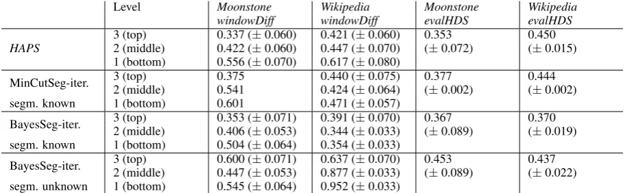
Table 2 shows the results of comparing HAPS with two baseline segmenters using windowDiff and evalHDS. HAPS was run without knowing the number of segments. MCSeg required that the exact number be specified. BSeg was tested with and without that parameter. Therefore, rows 3 and 4 in Table 2 correspond to baselines considerably more informed thanHAPS. This is especially true of the bottom levels where sometimes knowing the exact number of segments unambiguously determines the only possible segmentation.
The results suggest that HAPS performs well on theMoonstonedata even when compared to more informed baselines. This applies to both metrics, windowDiff and evalHDS. BSeg performs slightly better at the bottom levels of the tree when it has the information about the exact number of segments. We hypothesize that the advantage may be due to this additional information, especially when segmenting already small segments at level 1 into a predefined number of segments. Another explanation may be that when usingwindowDiff as the evaluation metric,HAPSwas fine-tuned so as to maximize the value ofwindowDiff at the top level, effectively disregarding lower levels of segmentation.
4When working with theMoonstonedataset, we realized that the software produces very low values, almost too good to be
true. That is because the bottommost annotations are very fine-grained. Sometimes each paragraph corresponds to a separate segment. This causes problems for the software. So, when we reportevalHDS values for theMoonstonedataset, we only consider two top levels of the tree, disregarding the leaves. We also remove the “too good to be true” outliers, though the “bad” tail is left intact. We applied the same procedure to all three segmenters, only for theMoonstonedataset.
Level Moonstone Wikipedia Moonstone Wikipedia
windowDiff windowDiff evalHDS evalHDS
HAPS 2 (middle)3 (top) 0.422 (0.337 (±±0.060)0.060) 0.421 (0.447 (±±0.060)0.070) 0.353(±0.072) 0.450(±0.015) 1 (bottom) 0.556 (±0.070) 0.617 (±0.080)
MinCutSeg-iter. 2 (middle)3 (top) 0.5410.375 0.440 (0.424 (±±0.075)0.064) 0.377(±0.002) 0.444(±0.002) segm. known 1 (bottom) 0.601 0.471 (±0.057)
BayesSeg-iter. 2 (middle)3 (top) 0.406 (0.353 (±±0.071)0.053) 0.391 (0.344 (±±0.070)0.033) 0.367(±0.089) 0.370(±0.019) segm. known 1 (bottom) 0.504 (±0.064) 0.354 (±0.033)
BayesSeg-iter. 2 (middle)3 (top) 0.447 (0.600 (±±0.071)0.053) 0.637 (0.877 (±±0.070)0.033) 0.453(±0.089) 0.437(±0.022) segm. unknown 1 (bottom) 0.545 (±0.064) 0.952 (±0.033)
Table 2: Evaluation ofHAPSand iterative versions ofAPS,MCSegandBSegusingwindowDiff per level (meanwindowDiff and standard deviation for cross-validation)
Moonstonecorpus Austen corpus
ROUGE-1 ROUGE-L ROUGE-1 ROUGE-L
Segment centres 0.341 0.321 0.291 0.301
(0.312, 0.370) (0.298, 0.346) (0.272, 0.311) (0.293, 0.330)
CohSum 0.294 0.269 0.305 0.307
summaries (0.243, 0.334) (0.226, 0.306) (0.290, 0.320) (0.287, 0.327)
Table 3: HAPSsegment centres compared toCohSumsummaries: ROUGE scores and 95% confidence intervals
All segmenters perform worse on the Wikipedia dataset. Using that scale, informedBSegperforms the best, but it is interesting to note a significant drop in performance when the number of segments is not specified.
Overall, HAPS appears to perform better than, or comparably to, the more informed baselines, and much better than the baseline not given information about the number of segments.
We also made a preliminary attempt to evaluate the quality of segment centres by comparing them to the summaries created by theCohSumsummarizer. In addition to working with theMoonstonecorpus, we collected a corpus of 20 chapters from various novels by Jane Austen.
Table 3 shows the results. They are not conclusive because there is no evidence that ROUGE scores correlate with the quality of automatically created summaries for literature. According to the scores in Table 3, however, the summaries created by CohSum cannot be distinguished from simple summaries composed of segment centres identified byHAPS. We interpret this as a sign that the centres identified byHAPSare approximately as informative as those created by an automatic summarizer.
7 A brief conclusion
This paper presented HAPS, a hierarchical segmenter for free text. Given an input document, HAPS creates a topical tree and identifies a segment centre for each segment. One of the advantages ofHAPS is that it does not require the exact number of segments in advance. Instead, it estimates the number of segments given information on generic preferences with regard to segmentation granularity. We also created a corpus of hierarchical segmentations which has been annotated by 3-6 people per chapter.
A Java implementation ofHAPSand theMoonstonecorpus are publicly available.6
Acknowledgements
We thank Chris Fournier (for computingSvalues using a beta version of SegEval software for hierar-chical datasets), Lucien Carrol (for help and discussion of theevalHDSsoftware and representation) and Christian Smith (for allowing us to use his implementation ofCohSum).
References
Christopher M. Bishop. 2006. Pattern Recognition and Machine Learning. Springer.
David Blei and Pedro Moreno. 2001. Topic segmentation with an aspect hidden Markov Model. InProceedings of the 24th Annual International ACM SIGIR Conference on Research and Development in Information Retrieval, pages 343–348.
Lucien Carroll. 2010. Evaluating Hierarchical Discourse Segmentation. InHuman Language Technologies: The 2010 Annual Conference of the North American Chapter of the Association for Computational Linguistics, pages 993–1001.
Lan Du, Wray Buntine, and Mark Johnson. 2013. Topic Segmentation with a Structured Topic Model. In
Proceedings of the 2013 Conference of the North American Chapter of the Association for Computational Linguistics: Human Language Technologies, pages 190–200, Atlanta, Georgia.
Jacob Eisenstein and Regina Barzilay. 2008. Bayesian Unsupervised Topic Segmentation. InProceedings of the 2008 Conference on Empirical Methods in Natural Language Processing, pages 334–343, Honolulu, Hawaii. Jacob Eisenstein. 2009. Hierarchical Text Segmentation from Multi-Scale Lexical Cohesion. InProceedings of
the 2009 Conference of the North American Chapter of the Association for Computational Linguistics: Human Language Technologies, pages 353–361. The Association for Computational Linguistics.
Vanessa Wei Feng and Graeme Hirst. 2012. Text-level Discourse Parsing with Rich Linguistic Features. In
Proceedings of the 50th Annual Meeting of the Association for Computational Linguistics (Volume 1: Long Papers), pages 60–68, Jeju Island, Korea, July. Association for Computational Linguistics.
Chris Fournier and Diana Inkpen. 2012. Segmentation Similarity and Agreement. InProceedings of the 2012 Conference of the North American Chapter of the Association for Computational Linguistics: Human Language Technologies, pages 152–161, Montr´eal, Canada.
Inmar E. Givoni, Clement Chung, and Brendan J. Frey. 2011. Hierarchical Affinity Propagation. InUncertainty in AI, Proceedings of the Twenty-Seventh Conference (2011), pages 238–246.
Aria Haghighi and Lucy Vanderwende. 2009. Exploring Content Models for Multi-Document Summarization. In
Proceedings of Human Language Technologies: The 2009 Annual Conference of the North American Chapter of the Association for Computational Linguistics, pages 362–370, Boulder, Colorado, June.
Marti A. Hearst. 1997. TextTiling: segmenting text into multi-paragraph subtopic passages. Computational Linguistics, 23(1):33–64.
Hugo Hernault, Helmut Prendinger, David A. duVerlea, and Mitsuru Ishizuka. 2010. HILDA: A Discourse Parser Using Support Vector Machine Classification. Dialogue and Discourse, 3:1–33.
Anna Kazantseva and Stan Szpakowicz. 2011. Linear Text Segmentation Using Affinity Propagation. In Proceed-ings of the 2011 Conference on Empirical Methods in Natural Language Processing, pages 284–293, Edinburgh, Scotland.
Anna Kazantseva and Stan Szpakowicz. 2012. Topical Segmentation: a Study of Human Performance and a New Measure of Quality. InProceedings of the 2012 Conference of the North American Chapter of the Association for Computational Linguistics: Human Language Technologies, pages 211–220, Montr´eal, Canada.
Anna Kazantseva. 2014. Topical Structure in Long Informal Documents. Ph.D. thesis, University of Ottawa.
hhttp://www.eecs.uottawa.ca/˜ankazant/i.
Chin-Yew Lin. 2004. ROUGE: A Package for Automatic Evaluation of summaries. In Text Summarization Branches Out, Proceedings of the ACL Workshop, pages 74–81, Barcelona, Spain.
Igor Malioutov and Regina Barzilay. 2006. Minimum Cut Model for Spoken Lecture Segmentation. In Pro-ceedings of the 21st International Conference on Computational Linguistics and 44th Annual Meeting of the Association for Computational Linguistics, pages 25–32, Sydney, Australia.
William C. Mann and Sandra A. Thompson. 1988. Rhetorical Structure Theory: Toward a functional theory of text organization. Text, 8(3):243–281.
Daniel Marcu. 2000.The Theory and Practice of Discourse Parsing and Summarization. MIT Press, Cambridge, Mass.
Rada Mihalcea and Paul Tarau. 2004. Textrank: Bringing order into texts. In Dekang Lin and Dekai Wu, editors,
Proceedings of the Conference on Empirical Methods in Natural Language Processing 2004, pages 404–411, Barcelona, Spain.
Hemant Misra, Franc¸ois Yvon, Olivier Capp´e, and Joemon M. Jose. 2011. Text segmentation: A topic modeling perspective. Information Processing and Management, 47(4):528–544.
Hyo-Jung Oh, Sung Hyon Myaeng, and Myung-Gil Jang. 2007. Semantic passage segmentation based on sentence topics for question answering. Information Sciences, an International Journal, 177:3696–3717.
Lev Pevzner and Marti A. Hearst. 2002. A Critique and Improvement of an Evaluation Metric for Text Segmenta-tion. Computational Linguistics, 28(1):19–36.
Jay M. Ponte and W. Bruce Croft. 1998. A Language Modeling Approach to Information Retrieval. InSIGIR ’98: Proceedings of the 21st Annual International ACM SIGIR Conference on Research and Development in Information Retrieval, pages 275–281, Melbourne, Australia.
Christian Smith, Henrik Danielsson, and Arne Jnsson. 2012. A more cohesive summarizer. In24th International Conference on Computational Linguistics, Proceedings of COLING 2012: Posters, pages 1161–1170, Mumbai, India.
Fei Song, William M. Darling, Adnan Duric, and Fred W. Kroon. 2011. An iterative approach to text segmentation. InProceedings of the 33rd European Conference on Advances in Information Retrieval, ECIR’11, pages 629– 640, Berlin, Heidelberg. Springer-Verlag.
Florian Wolf and Edward Gibson. 2006. Coherence in Natural Language: Data Structures and Applications. MIT Press, Cambridge, MA.
Yaakov Yaari. 1997. Segmentation of Expository Texts by Hierarchical Agglomerative Clustering. InProceedings of International Conference on Recent Advances in Natural Language Processing RANLP97, pages 59–65, Tzigov Chark, Bulgaria.