Relational machine learning for electronic health record-driven phenotyping

Relational machine learning for electronic health record-driven

phenotyping

Peggy L. Peissig

_{, Vitor Santos Costa}

_{, Michael D. Caldwell}

_{, Carla Rottscheit}

_{, Richard L. Berg}

_,

Eneida A. Mendonca

, David Page

a

Biomedical Informatics Research Center, Marshfield Clinic Research Foundation, Marshfield, WI, USA b_{DCC-FCUP and CRACS INESC-TEC, Department de Ciência de Computadores, Universidade do Porto, Portugal} c

Department of Surgery, Marshfield Clinic, Marshfield, WI, USA d

Department of Biostatistics and Medical Informatics, University of Wisconsin–Madison, USA e

Department of Pediatrics, University of Wisconsin–Madison, USA f

Department of Computer Sciences, University of Wisconsin–Madison, USA

a r t i c l e

i n f o

Article history:

Received 27 February 2014 Accepted 8 July 2014 Available online 15 July 2014 Keywords:

Machine learning Electronic health record Inductive logic programming Phenotyping

Relational machine learning

a b s t r a c t

Objective:Electronic health records (EHR) offer medical and pharmacogenomics research unprecedented opportunities to identify and classify patients at risk. EHRs are collections of highly inter-dependent records that include biological, anatomical, physiological, and behavioral observations. They comprise a patient’s clinical phenome, where each patient has thousands of date-stamped records distributed across many relational tables. Development of EHR computer-based phenotyping algorithms require time and medical insight from clinical experts, who most often can only review a small patient subset repre-sentative of the total EHR records, to identify phenotype features. In this research we evaluate whether relational machine learning (ML) using inductive logic programming (ILP) can contribute to addressing these issues as a viable approach for EHR-based phenotyping.

Methods: Two relational learning ILP approaches and three well-known WEKA (Waikato Environment for Knowledge Analysis) implementations of non-relational approaches (PART, J48, and JRIP) were used to develop models for nine phenotypes. International Classification of Diseases, Ninth Revision (ICD-9) coded EHR data were used to select training cohorts for the development of each phenotypic model. Accuracy, precision, recall, F-Measure, and Area Under the Receiver Operating Characteristic (AUROC) curve statistics were measured for each phenotypic model based on independent manually verified test cohorts. A two-sided binomial distribution test (sign test) compared the five ML approaches across phe-notypes for statistical significance.

Results: We developed an approach to automatically label training examples using ICD-9 diagnosis codes for the ML approaches being evaluated. Nine phenotypic models for each ML approach were evaluated, resulting in better overall model performance in AUROC using ILP when compared to PART (p= 0.039), J48 (p= 0.003) and JRIP (p= 0.003).

Discussion: ILP has the potential to improve phenotyping by independently delivering clinically expert interpretable rules for phenotype definitions, or intuitive phenotypes to assist experts.

Conclusion:Relational learning using ILP offers a viable approach to EHR-driven phenotyping.

Ó2014 Elsevier Inc. All rights reserved.

1. Introduction

Medical research attempts to identify and quantify relation-ships between exposures and outcomes. A critical step in this

process is subject characterization orphenotyping[1–4]. Without rigorous phenotyping, these relationships cannot be properly assessed, leading to irreproducible study results and associations

[1]. With the proliferation of electronic health records (EHRs), com-puterized phenotyping has become a popular and cost effective approach to identify research subjects[5]. The EHR contains highly inter-dependent biological, anatomical, physiological, and behav-ioral observations, as well as facts that represent a patient’s diagnosis and medical history. Typically, developing EHR-based

http://dx.doi.org/10.1016/j.jbi.2014.07.007

1532-0464/Ó2014 Elsevier Inc. All rights reserved.

⇑Corresponding author. Address: Biomedical Informatics Research Center, Marshfield Clinic Research Foundation, 1000 N. Oak Avenue (ML8), Marshfield, WI 54449, USA. Fax: +1 (715) 221 6402.

E-mail address:peissig.peggy@marshfieldclinic.org(P.L. Peissig).

Contents lists available atScienceDirect

Journal of Biomedical Informatics

phenotyping algorithms requires conducting multiple iterations of selecting patients from the EHR and then reviewing the selections to identify classification features that succinctly categorize them into study groups[6]. This process is time consuming[1]and relies on expert perceptions, intuition, and bias. Due to time limitations, experts carefully examine a small fraction of available EHR data for phenotype development. In addition, due to both the enormous volume of data found in the EHR and human bias, it is difficult for experts to uncover ‘‘hidden’’ relationships or ‘‘unseen’’ features relevant to a phenotype definition. The result is a serious temporal and informative bottleneck when constructing high quality research phenotypes.

The use of machine learning (ML) as an alternative EHR-driven phenotyping strategy has been limited[7–13]. Previous ML studies have applied a variety of standard approaches (e.g. SMO, Ripper, C4.5, Naïve Bayes, Random Forest via WEKA, Apriori, etc.) to coded EHR data in order to identify relevant clinical features or rules for phenotyping. All of these ML methods werepropositional, that is, they used data that were placed into a single fixed length, flat fea-ture table for analysis.

Data from EHRs pose significant challenges for such proposi-tional ML and data mining approaches, as previously noted[14]. First, EHRs may include reports on thousands of different condi-tions across several years. Knowing which features to include in the final feature table and how they relate often requires clinical intuition and a considerable amount of time spent by experts (phy-sicians). Second, EHR data are noisy. For example, in some cases diagnostic codes are assigned to explain that laboratory tests are being done to confirm or eliminate the coded diagnosis, rather than to indicate that the patient actually has the diagnosis. Third, EHR data are highly relational and multi-modal. Known flattening tech-niques, such as computing summary features or performing a data-base join operation, can usually result in loss of information[15]. For example, the Observational Medical Outcomes Partnership (OMOP) phenotypes lymphoma as either a temporal sequence ini-tiated with a biopsy or related procedure, followed within 30 days by a 200-202 International Classification of Diseases, Ninth Revi-sion (ICD-9) code, or a 200-202 ICD-9 code followed within 30 days by radiation or a chemotherapeutic treatment[16]. Verifying such a rule requires using data from three different tables and compar-ing the respective event times. Thus, a flat feature representation for learning ignores the structure of EHR data and, therefore, does not suitably model this complex task. Arguably, more advanced data structures such as trees, graphs, and propositional reasoners can handle the EHR data structure, but these approaches assume a noise free domain and cannot deal with missing or disparate data often present in the EHR[17,18].

Inductive logic programming (ILP), a subfield of relational machine learning, addresses the complexities of dealing with multi-relational EHR data[15]and has the potential to learn fea-tures without the existential perceptions of experts. ILP has been used in medical studies ranging from predictive screening for breast cancer [19,20] to predicting adverse drug events

[14,21,22]or adverse clinical outcomes[23–25]. Unlike rule induc-tion and other proposiinduc-tional machine learning algorithms that assume each example is a feature vector or a record, ILP algorithms work directly on data distributed over different EHR tables. The algorithmic details of leading ILP systems have been thoroughly described[26,27]and are summarized in the methods section.

To our knowledge, this represents the first use of ILP for pheno-typing. The work of Dingcheng et al. in phenotyping type 2 diabe-tes[11] is similar to ours in that it also uses a rule-based data-mining approach (Apriori association rule learning algorithm) which shares the advantage of learning rules for phenotyping that are easily understood by human users. The primary difference between the two approaches is our use of ILP to directly learn from

the extant tables of the EHR versus Apriori, which must learn from data conflated into a single table. This paper compares the use of ILP for phenotyping to other well-known propositional ML approaches.

As a final contribution, we introduce several novel techniques used to better automate the learning process and to improve model performance. These techniques fall into three categories: (1) selection of training set examples without expert (physician) involvement to provide supervision for the learning activities; (2) left-censoring of background data to identify subgroups of patients that have similar features denoting the phenotype; and (3) infusing borderline positive examples to improve rule prediction.

2. Methods

The Marshfield Clinic Research Foundation’s Institutional Review Board approved this study. The goal of our research was twofold: (1) to evaluate the performance of ILP for EHR-driven phenotyping and compare it to other ML and data mining approaches; and (2) to develop methods that reduce expert (phy-sician) time and enhance attribute awareness in the EHR-driven phenotyping process. The methods presented in this paper were applied to nine disease-based phenotypes to demonstrate the util-ity of the ILP approach.

2.1. Data source, study cohort, and phenotype selection

Marshfield Clinic’s internally developed CattailsMD EHR-Research Data Warehouse (RDW) was used as the source of data for this investigation. RDW data from 1979 through 2011, includ-ing diagnoses, procedures, laboratory results, observations, and medications for patients residing in a 22 ZIP Code area, were de-identified and made available for this study. The phenotypes used in this investigation were selected based on the availability of manually validated (case-control status) cohorts and include: acute myocardial infarction, acute liver failure, atrial fibrillation, cataract, congestive heart failure, dementia, type 2 diabetes, dia-betic retinopathy and deep vein thrombosis[24,25,28]. The RDW was used to select training cohorts for each phenotype. These training cohorts were used to guide phenotype model develop-ment for all of the ML approaches. The manually validated cohorts (henceforth referred to as testing subjects or test cohorts) were used to test the phenotype models by providing model perfor-mance comparison statistics. An overview of the study design is presented inFig. 1.

2.2. Identification of training set examples

The ability to accurately identify training examples to guide a supervised machine learning task is critical. Several ML studies have used experts (physicians) to review medical records to clas-sify patients into the positive (POS) (patients with a condition or exposure) and NEG (patients without the condition) example cate-gories [7,9] or used pre-existing validated cohorts representing POS and NEG training examples. A secondary goal of this research was to develop methods that could reduce expert (physician) time required for EHR-driven phenotyping; thus, it would be optimal to develop an approach for selecting training examples that did not require physician input or pre-existing categorized training examples.

A recent study by Carroll et al.[7] evaluated support vector machines for phenotyping rheumatoid arthritis and demonstrated the utility of ICD-9 CM diagnostic codes when characterizing research subjects. This knowledge coupled with our past pheno-typing experience [28] prompted the use of ICD-9 codes as a

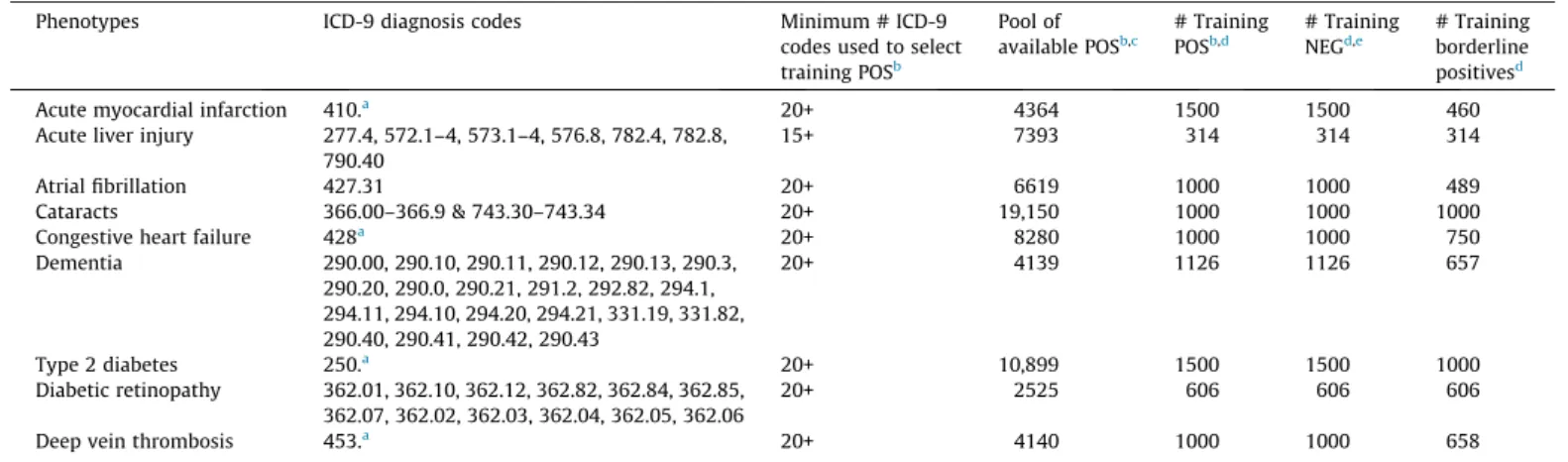
possible surrogate to identify potential positive (POS) training examples for model building. A sampling frame of patients with at least 15-20 ICD-9 codes spanning multiple days was used to define the surrogate POS cohort. From this cohort, we randomly selected a subset for model building (henceforth referred to as the POS training set). We required multiple ICD-9 codes based on the assumption that a patient who truly exhibits one of the pheno-types of interest will receive continuing care, in contrast with a patient who does not exhibit the phenotype but may have a small number of relevant ICD-9 codes in their record for administrative/ billing reasons. A working cutoff for the number of codes was established as follows. The frequency distribution of patient num-bers of ICD-9 codes was determined. Ranking patients from highest to lowest number of ICD-9 diagnoses, we targeted between 1000 and 1500 patients with highest ICD-9 counts to be labeled as POS, and similarly placed an upper limit on the training set size (refer toTable 1) to facilitate timely data transfers between the RDW and the machine learning environment.

For each selected POS in our training set, we randomly selected a NEG (ICD-9 code of the phenotype was not present in patient’s medical history) from a pool of similar age and gender matched patients (Fig. 2 provides overview of the sampling strategy). Patients with only a single diagnosis or multiple diagnoses on the same day were labeled as borderline positive examples (BPs). The use of these classifications will be described later. Refer to

Table 1 for details on POS, NEG and BP numbers for each phenotype.

2.3. Identification of testing set examples

Earlier in this discussion we indicated that we had access to manually validated phenotyped cohorts. We chose to use these cohorts for testing the performance of the phenotype models rather than for model training or development. Two testing cohorts (congestive heart failure [CHF] and acute liver injury [ALI]) were constructed in parallel to this investigation. A similar manual chart review and classification process was used for each phenotype to construct the testing cohorts. In general, trained research coordina-tors manually reviewed charts and classified a list of patients as either POS or NEG. A second research coordinator independently reviewed a sample of records completed by the first reviewer

(usually a 5–10% sample or a fixed sample size for the larger cohorts) for quality assurance. A board-certified physician resolved disagreements or questions surrounding the classifications of subjects. For example, there were three noted disagreements in the ALI abstraction that were resolved in this manner.

2.4. Machine learning phenotyping approaches 2.4.1. ILP approach

ILP addresses the problem of learning (or inducing) first-order predicate calculus (FOPC) rules from a set of examples and a data-base that includes multiple relations (or tables). Most work in ILP limits itself to non-recursive Datalog[29], a subset of FOPC equiv-alent to relational algebra expressions or SQL queries, which differ-entiate positive examples (cases) from negative examples (control patients) given background knowledge (EHR data). A database with multiple tables is represented as an extensional Datalog program, with one predicate for each table and one fact for each tuple (record) in each table. The rules that we learn are equivalent to SQL queries; hence, a rule can be thought of as defining a new table and a set of rules as defining a new view of the database.

Our work used Muggleton’s Progol algorithm [30] as imple-mented in Srinivasan’s Aleph system[31].Progolapplies the idea that if a rule is useful, it must explain (or cover) at least one exam-ple. Thus, instead of blindly generating rules,Progolfirst looks in detail at one example, and it only constructs rules that are guaran-teed to cover that example. The benefit of using this approach is that instead of having to generate rules for all conditions, drugs, or labs in the EHR, it can generate rules for a much smaller number of conditions.

The Aleph implementation uses the data connected to an exam-ple to construct rules. The head of the rule always refers to the patient. The body refers to facts for that specific patient. These ‘‘ground’’ rules are then generalized by introducing variables au lieu of individual patients or of specific time points. Shorter rules are constructed first. In this study, we used breadth-first search over a fast-growing search space, so the major limitation is the number of elements that we combine and still achieve acceptable performance. This is rarely more than 4. It is possible to explore longer rules, often up to 10 or more, by using greedy search or ran-domized search instead of a complete search.

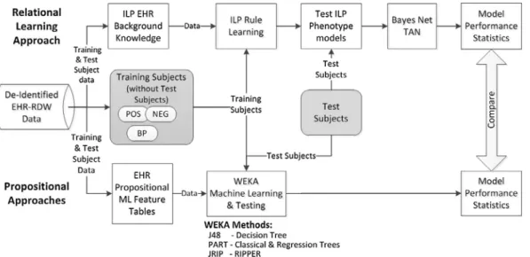
Fig. 1.Overview of data preparation and analysis processes. Positive (POS), negative (NEG) and borderline positive (BP) training examples are selected using the electronic health record (EHR) data. Inductive logic programming (ILP) background knowledge (EHR data) and propositional machine learning (ML) feature tables are created and used by each of the respective ML methods. Manually verified test subject data is prepared similar to training data and is used to create performance statistics that are used to compare ML approaches.

In a nutshell, theProgol/Alephalgorithm: (1) Selects a positive example (referred to as a seed) not yet explained by any rule. In the EHR domain, the positive example is a patient that has the exposure or medical condition of interest. (2) Searches the data-base for data directly related to the example. In the case of an EHR, this means collecting all diagnoses, prescriptions, lab results, etc., for the example patient. (3) Generates rules based on the patient. The rule will be constructed from the events of the chosen patient’s history (referred to as clauses) generalized to explain other patients. This is achieved by replacing the references to the actual patient and temporal data with variables. The resulting rule

(with variables) is applied to the training examples (both positive and negative) using the EHR data to identify patients that can be explained by the rule. (4) In practice, ILP must deal with inconsis-tent and incomplete data; hence, it uses statistical criteria based on the number of positively and negatively explained examples to determine the quality of the rule. Two simple criteria that are often used to score rules are precision (the fraction of covered examples that are positive, also called the positive predictive value) or the number of positive examples minus the number of negative exam-ples covered by the clause, known as coverage. (5) The procedure stops when it finds a good rule, and the examples explained by

Table 1

Phenotypes and sampling frame.

Phenotypes ICD-9 diagnosis codes Minimum # ICD-9 codes used to select training POSb Pool of available POSb,c # Training POSb,d # Training NEGd,e # Training borderline positivesd

Acute myocardial infarction 410.a _{20+ 4364 1500 1500 460}

Acute liver injury 277.4, 572.1–4, 573.1–4, 576.8, 782.4, 782.8, 790.40

15+ 7393 314 314 314

Atrial fibrillation 427.31 20+ 6619 1000 1000 489

Cataracts 366.00–366.9 & 743.30–743.34 20+ 19,150 1000 1000 1000

Congestive heart failure 428a

20+ 8280 1000 1000 750 Dementia 290.00, 290.10, 290.11, 290.12, 290.13, 290.3, 290.20, 290.0, 290.21, 291.2, 292.82, 294.1, 294.11, 294.10, 294.20, 294.21, 331.19, 331.82, 290.40, 290.41, 290.42, 290.43 20+ 4139 1126 1126 657 Type 2 diabetes 250.a 20+ 10,899 1500 1500 1000 Diabetic retinopathy 362.01, 362.10, 362.12, 362.82, 362.84, 362.85, 362.07, 362.02, 362.03, 362.04, 362.05, 362.06 20+ 2525 606 606 606

Deep vein thrombosis 453.a _{20+ 4140 1000 1000 658}

Note:Phenotype models were constructed for nine conditions. Training positive and borderline positive examples were identified using ICD-9 diagnosis codes. Negative training examples had no ICD-9 diagnosis code.

a

Include all decimal digits. b

POS indicates positive examples. c

Includes all patients with at least one ICD-9 diagnosis code. d

Randomly selected. e

NEG indicates negative examples.

Fig. 2.(A) Inductive logic programming (ILP) uses retrospective data to predict disease outcomes. (B) Phenotyping with ILP uses data collected after the incident date (of a condition), to predict features that a subgroup may be sharing that are representative of a phenotype.

the new rule are removed. If no more examples remain, learning is complete. Otherwise, the process is repeated on the remaining examples.Appendix A provides a more detailed introduction on ILP to assist readers’ understanding.

2.4.1.1. Traditional ILP use. ILP usage in the medical domain has focused on predicting patient outcomes [14,19–22]. Supervision for the prediction task comes from positive examples (POS—patients with a medical outcome) and negative examples (NEG—patients without the medical outcome), given some common exposure. For example, to develop a model that will predict diabetic retinopathy (DR), given a patient has diabetes, the supervision comes in the form of POS (diabetic patients that have DR) and NEG (diabetic patients without DR). EHR data collected before the DR occurrence is used to build a model to predict whether a diabetic patient is at future risk for DR (refer toFig. 2A).

2.4.1.2. ILP for phenotyping. ILP applied to the phenotyping task uses a similar approach, but in a reversed manner. For example, when phenotyping we should not assume that we know all the clinical attributes that are needed to succinctly identify patients with a given phenotype (e.g., diabetes). Suppose we do not know in advance that diabetes is associated with elevated blood sugar. The POS and NEG cannot be selected as training examples based on elevated blood sugar, because it is not yet known that elevated blood sugar is an indicator for diabetes. Instead, the problem can be addressed by selecting training examples based on the desired phenotype or disease outcome (diabetes) and then running ILP with EHR data filtered by dates occurring on or after the first diag-nosis (refer toFig. 2B). This seems counter-intuitive, because we are training on patients with data obtained after diabetes is diag-nosed in order to identify the common features of the phenotype (diabetes). The features (or ILP rules) can then be applied to retro-spective EHR data to select (or phenotype) unclassified patients. In addition, if we can identify diabetic patients based on similar med-ical features existing after the initial diagnosis, we may also be able to uncover unknown (unbiased) features that further define the phenotype.

2.4.1.3. Constructing background knowledge for ILP. Background

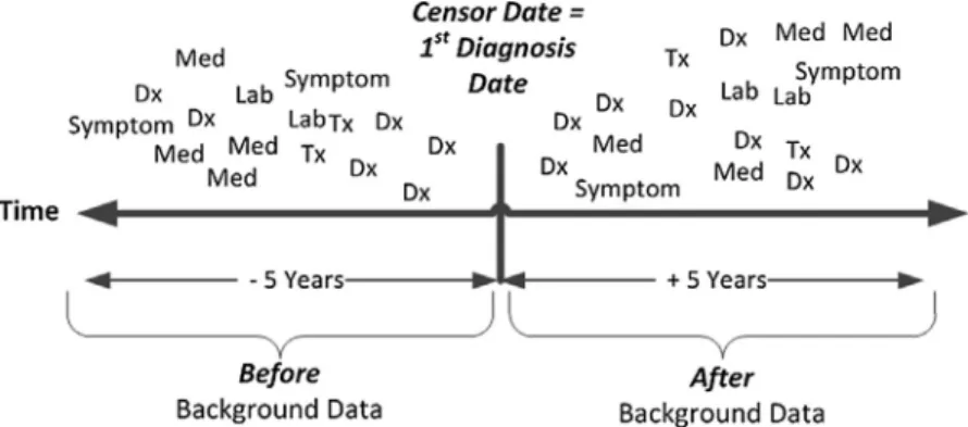
knowledge (EHR data) for phenotyping was created by selecting coded ICD-9 diagnosis, medication, laboratory, procedure, and biometric observation measurement records from the EHR. A cen-sor date, representing the initial diagnosis date of the phenotype, was determined for each POS and borderline positive (BP) example (BP will be explained in the following section). All EHR background knowledge records were labeled asbeforeorafter, based on the rela-tionship of the event date (date of diagnosis, procedure, lab, or med-ication) to the censor date (refer toFig. 3). Beforerecords were labeled if they occurred 5 years to 30 days before the censor date.

We used 30 days before the censor date, because we did not want to include EHR facts that might be associated with diagnosing the phenotype condition.Afterrecords were labeled if they occurred in the period from less than 30 days before the censor date through 5 years after the censor date. EHR background knowledge records for each NEG were similarly labeled asbeforeorafterbased on the censor date of the corresponding POS (since NEGs have no incident diagnosis date). All EHR background knowledge records were for-matted for Aleph ILP system software. The detailed methods sur-rounding background file creation can be found inAppendix B-3.

Appendix Cprovides detailed examples of diagnosis, lab, gender, drug, procedure, vitals and symptom record formatting for Aleph. To summarize, a ‘‘b’’ is attached to the beginning of the patient_id (first variable in the parentheses) to indicate abeforerecord (i.e. vitals(‘b222aaa222’,68110,’Blood Pressure Diastolic’,’60’). There is no prefix used when formatting the after record (i.e. vital-s(‘222aaa222’,78110,’Blood Pressure Diastolic’,’60’).

2.4.1.4. ILP scoring functions.Scoring functions in Aleph and other ILP systems evaluate the quality of a rule and thus, are fundamen-tal to the learning process. We tested two different scoring func-tions with Aleph[31]. The first scoring function follows standard ILP practice and was (POS(after) NEG(after)), where POS(after)

denotes positive examples that use EHR data after the censor date and NEG(after)denotes negative examples that use EHR data

after the censor date (Fig. 3). Simultaneously, we evaluated

(POS(after) (NEG(after)+ POS(before))), in which POS(before) denotes

positive examples that use EHR records before the censor date and POS(after)and NEG(after)are as in the previous example. Early

on we found that diagnoses tended to ‘‘follow’’ patients over time. The scoring function mimics an epidemiology research method calledCase-Crossoverstudy design, where each case serves as its own control and allows for the detection of differences from one time period to another[32]. In our example, the later scoring func-tion helps to identify differences in medical events between POS(after)and POS(before)time periods, thus highlighting new

medi-cal events that occurred after the initial diagnosis but not before. The cost function (POS(after) (NEG(after)+ POS(before))) was found

to improve model performance and accuracy over the initial scor-ing function. Henceforth, this function will be referred to asILP-1. From previous work, we found that using theILP-1scoring func-tion tended to create rules that could differentiate the POS and NEGs based on ICD-9 codes relatively well, but often failed to pro-vide more specific rules that could discriminate borderline POS and NEG examples. To further discriminate and improve the rules, we infused the NEGs with subjects that we considered borderline pos-itives (BPs). BPs are examples of patients that have one relevant diagnosis code, but not two, or several diagnoses on the same day with no subsequent follow-up. BPs are problematic because subjects may (or may not) have the medical diagnosis. This is

because ICD-9 diagnosis codes are sometimes used in clinical prac-tice to justify laboratory tests or procedures rather than to define that a patient has the diagnosis. BPs likely include patients that do not have the phenotype condition and by adding them to the NEGs, we increase the precision of the learned rules. The scoring function used to support the infusion of BPs into the NEGs is: (POS(after) (NEG(after)+ POS(before)+ BPs(after))). Henceforth, this

function will be referred to asILP + BP.

We used a 1:1 ratio of POS to NEG while building the phenotype model. Initially, we limited the number of POS and NEG to the maximum number of BPs available (this was done for ALI and dia-betic retinopathy phenotypes). Later, after completing a sensitivity analysis to determine the optimal percent of BPs to add to the NEGs (e.g., 25%, 50%, 75%, or 100%), we increased POS and NEG training sets selection to accommodate the maximum subject limit between 3–4000. The number of BPs used in each study was deter-mined by either the availability of BPs in the cohort, or the number of BPs could not exceed the number of NEG subjects in the training set. Refer toTable 1 for the exact number of diagnoses used to select training examples and the numbers of POS, NEG, and BPs present in each phenotype training set.

2.4.1.5. ILP configuration. ILP was adapted for phenotyping by

adjusting Aleph parameters reflecting the following beliefs: (1) accepted rules should cover very few, ideally zero, negative exam-ples; (2) rules that succeed on very few examples tend to over fit (a useful heuristic is that a rule is only acceptable when it covers at least 20 examples); and (3) search time heavily depends on the maximum number of rules that are considered for each seed. Because of the high run-time for relational learning and the large number of parameters, as well as to keep the process as simple and generalizable as possible, we did not tune, but rather chose a single set of parameter settings and applied them to all pheno-types. We were careful to avoid the pitfall of trying many combina-tions of parameter settings and then selecting the one that gives the best results on the test set. We instead chose to use the follow-ing settfollow-ings which had shown good performance in previous appli-cations: noise = 1, minpos = 80, minacc = 80, clause length = 4, caching = false, i = 3, record = true and nodes = 1,000,000.

Using the cataract phenotype as an example, we have presented a detailed description of our methods in Appendix Band made available examples of record formats.Appendix C has examples of the scripts and configuration files (cat.b – file that contains the parameters for running Aleph and runAleph.sh – a script that initi-ates the Aleph phenotype model building session).Appendix Dhas examples of ILP rules created for the cataract phenotype using ILP-1 and ILP + BP ML approaches.

2.4.2. Propositional machine learning approaches

We selected two popular ML classifiers available in the widely used Waikato Environment for Knowledge Analysis (WEKA) soft-ware [33], after conducting a sensitivity analysis (using several ML classifiers), to determine the highest performing approaches based on area under the receivers operating characteristics curve (AUROC). Using atrial fibrillation as the phenotype, we compared:

Random Forest(AUROC = 0.682),SMO(0.506),PART(0.772), andJ48

(0.772). From this analysis, we selectedJ48andPARTfor use in the ILP comparison.J48is based on a Java implementation of the well-known decision tree classifier C4.5[34]andPART, is the Java imple-mentation of a rule based classifier based on Classical and Regres-sion Tree[35]. We also selectedJRIP, the WEKA implementation of the propositional rule learner Repeated Incremental Pruning to Produce Error Reduction (RIPPER)[36]. The RIPPER implementa-tion is similar to ILP, except that it assumes that each example is a feature vector or record versus ILP algorithms work directly on data distributed over multiple tables.

2.4.2.1. Feature table creation. A feature table consisting of the same POS and NEG examples used in ILP phenotype model building was created and used by the propositional ML approaches for each phe-notype. A record for each subject was constructed using information obtained from the EHR. Each unique occurrence of a diagnosis, lab-oratory result (categorized as ‘above’, ‘within’ or ‘below’ the normal range), medication, or procedure was identified as a feature. Fre-quencies of occurrence were calculated for each feature by subject. Because of the large size of the feature table, we only used features that were shared by more than 0.25% of the training subjects. In other words, features were included if more than two or three sub-jects (depending on phenotype) had the feature. The same features identified for the training sets were used as features for the valida-tion/test examples. For details refer toAppendix B.7.

2.5. Analysis

Phenotyping model performance measurements were calcu-lated using the number of correctly classified testing subjects. Con-tingency tables were used to calculate accuracy, precision, recall (the true positive rate, also called sensitivity), and F-Measure (defined as 2[(recallprecision)/(recall + precision)]) statistics for the ILP models. WEKA, version 3.6.9, automatically calculated those statistics along with Receiver Operator Characteristic (ROC) curves and area under the ROC curve (AUROC), for the proposi-tional ML methods (J48, PART, and JRIP). To associate the probabil-ities of AUROC and construct ROC curves for the ILP models, we built a feature table using the ILP rules as features. A binary code indicating if a subject met (or not), the rule criteria was assigned for each feature by subject in the testing cohort. The Bayes Net-Tan classifier, as implemented in WEKA, was used to calculate AUROC using the ILP features (rules) for each phenotype model

[37]. Such use of a Bayesian network to combine relational rules learned by ILP is a popular approach used in statistical relational learning to gain ROC curves and AUROC[15].

Significance testing using a two-sided sign test (binomial distri-bution test) at 95% confidence was used to evaluate model sensi-tivity when adding varying percentages of BPs (25%, 50%, 75%, and 100%) to NEGs in the ILP + BP scoring function. Discordant clas-sifications of POS and NEG were obtained for each ILP approach comparison and then similar significance testing conducted.

To assess the difference in overall ML approach performance, we counted the number of wins for a ML approach across pheno-types and compared it to the number of wins for the comparison ML approach. Significance testing was done using a two-sided sign test (binomial distribution test) at 95% confidence, to evaluate a difference in overall model performance between any of the ILP-1, ILP + BP, PART, J48, and JRIP models.

3. Results

The sampling frame used for the selection of all phenotype training sets consisted of 113,493 subjects. Table 1provides the number of POS, NEG, and BP training subjects randomly selected and used for the development of each phenotype model. Training set sizes for both POS and NEG examples ranged from 314 (acute liver injury) to 1500 (acute myocardial infarction and type 2 diabetes).

There was no significant difference detected in overall model performance when adjusting the BP percentages (between 25%, 50%, 75%, and 100%) for the ILP + BPscoring function. We found that adding BP examples to the scoring function yielded more descriptive rules for all phenotypes. For example, using atrial fibril-lation, a single rule having the presence of ICD-9 code ‘427.31’ (atrial fibrillation) was learned by theILP-1 approach. Using the

ILP + BPwith the addition of BPs at 50%, presented a total of 58 rules, which included a combination of diagnoses, labs, procedures, medications, and age. For consistency in reporting results, hence-forth we will useILP + BPwith the contribution of 50% BPs.

Table 2provides descriptive information on the phenotype test-ing cohorts. The POS and NEG testtest-ing cohorts tended to be older (>65 years of age) and similar with respect to years of follow-up and ICD-9 diagnosis counts.

Table 2

Validation-testing sample characteristics.

Phenotypes Total number Mean Years followup4

(St Dev) ICD-9 diagnosis count (St Dev) POSa NEGb Female (%) Agec POSa NEGb POSa NEGb Acute myocardial infarction 363 158 199 (38.2%) 73.8 37.9 (9.7) 33.5 (12.2) 1848 (1475) 1384 (1304) Acute liver injury 44 6 23(46%) 69.3 34.9 (10.6) 35.2 (10.0) 1880 (1568) 2550 (951) Atrial fibrillation 36 35 31 (44%) 79.8 29.2 (13.1) 31.7 (14.5) 1345 (811) 1468 (1100) Cataracts 244 110 210 (59.32%) 75.2 39.7 (9.8) 37.9 (11.2) 1395 (1004) 864 (616) CHF 60 36 51 (52%) 70 35.4 (10.0) 26.1 (13.8) 1614 (1184) 623 (647) Dementia 303 70 203 (54.4%) 84 36.9 (11.3) 37.4 (8.64) 1579 (980) 1438 (1067) Type 2 diabetes 113 52 99 (60%) 67 36.3 (12.3) 34.0 (13.6) 1447 (781) 925 (781) Diabetic retinopathy 40 46 39 (45.4%) 71.6 35.1 (12.7) 37.9 13.8) 2032 (1158) 1614 (1158) Deep vein thrombosis 217 870 614 (56%) 76 38.3 (9.9) 38.9 (10.2) 1947 (1604) 1269 (836) Note:Phenotype models were validated using these validation cohorts.

a_{POS indicates positive examples.} b _{NEG indicates negative examples.} c

Mean age calculated by (year of data pull (2012) – birth year). d

Years follow-up calculated by determining difference between first and last diagnosis date.

Table 3

Phenotype model validation results by phenotype. Phenotype Acute myocardial infarction Acute liver injury Atrial fibrillation

Cataracts CHF Dementia Type 2 diabetes Diabetic retinopathy Deep vein thrombosis Accuracy ILP-1a 0.800 0.600 0.775 0.890 0.865 0.810 0.939 0.977 0.980 ILP + BPb 0.810 0.640 0.732 0.898 0.885 0.810 0.945 0.988 0.965 PARTc _{0.775 0.660 0.775 0.879 0.875 0.850 0.945 0.988 0.949} J48d 0.785 0.700 0.775 0.822 0.875 0.834 0.945 0.988 0.949 JRIPe 0.791 0.780 0.775 0.879 0.875 0.807 0.945 0.988 0.981 Precision ILP-1a _{0.863 0.929 0.700 0.865 0.831 0.858 0.919 0.952 0.990} ILP + BPb _{0.877 0.906 0.689 0.877 0.855 0.936 0.926 0.976 0.954} PARTc 0.790 0.848 0.824 0.877 0.811 0.859 0.949 0.989 0.949 J48d 0.797 0.829 0.824 0.819 0.881 0.850 0.949 0.989 0.949 JRIPe 0.869 0.902 0.700 0.904 0.853 0.917 0.926 0.976 0.990 Recall ILP-1a 0.850 0.591 0.972 0.996 0.980 0.858 1.000 1.000 0.910 ILP + BPb 0.850 0.659 0.860 0.992 0.980 0.822 1.000 1.000 0.870 PARTc 0.755 0.660 0.775 0.879 0.875 0.850 0.945 0.988 0.949 J48d 0.785 0.700 0.755 0.822 0.875 0.834 0.945 0.988 0.960 JRIPe 0.824 0.841 0.972 0.922 0.967 0.838 1.000 1.000 0.912 F-Measure ILP-1a 0.856 0.722 0.813 0.926 0.900 0.858 0.958 0.976 0.947 ILP + BPb 0.879 0.763 0.795 0.939 0.914 0.894 0.961 0.988 0.940 PARTc 0.788 0.719 0.765 0.877 0.871 0.854 0.944 0.988 0.949 J48d _{0.789 0.747 0.765 0.820 0.871 0.840 0.944 0.988 0.960} JRIPe _{0.794 0.798 0.765 0.878 0.871 0.818 0.944 0.988 0.980} AUROCh ILP-1 + BNTf 0.769 0.752 0.772 0.893 0.825 0.817 0.904 0.991 0.953 ILPBP + BNTg _{0.831 0.701 0.774 0.873 0.914 0.831 0.957 0.990 0.971} PARTc _{0.788 0.716 0.772 0.842 0.844 0.798 0.913 0.989 0.947} J48d 0.722 0.619 0.722 0.783 0.844 0.766 0.913 0.989 0.927 JRIPe 0.769 0.587 0.772 0.852 0.844 0.755 0.913 0.989 0.955

Boldednumbers indicate highest score between phenotyping methods.

Note:Phenotype model accuracy measurements were calculated for each scoring function by using the number of correctly classified positive and negative validation examples.

a_{ILP-1:inductive logic programming with using POS(after) (NEG(after) + POS(before));} b

ILP + BP:inductive logic programming + borderline positives using POS(after) (NEG(after) + POS(before) + FP(after)). c

PART:Java implementation of a rule based classifier in WEKA. d

J48:Java implementation of C4.5 classifier available in WEKA. e

JRIP:Java implementation of RIPPER classifier available in WEKA. f

ILP-1 + BNT:BayesNet-Tan using ILP classification rules. g

ILPBP + BNT:BayesNet-Tan using ILP + BP classification rules. h

Fig. 4.A comparison between all machine learning approaches by phenotype using receiver operator characteristic (ROC) curves. The diabetes retinopathy ROC curves are not displayed because of the similarity between each machine learning approach. Overall, the pictured models were very similar with ILP + BP ROC showing the best results for congestive heart failure, deep vein thrombosis and type 2 diabetes.

Nine phenotypes were modeled with the performance mea-surements for each ML approach (ILP-1, ILP + BP,PART, J48, and

JRIP) appearing inTable 3. Type 2 diabetes, diabetic retinopathy, and deep vein thrombosis phenotypic models consistently had high performance statistics (>0.900 in all categories) across all ML approaches. Acute liver injury had the lowest performance measurements for all ML approaches. There was no significant dif-ference in overall accuracy between ILP-1 and ILP + BP models, although ILP-1 performed significantly better than ILP + BP in detecting POS examples (p= 0.0006), andILP + BPperformed sig-nificantly better than ILP-1 when detecting NEG examples (p= 0.008). The addition of BP examples had the desired effect of increasing precision, but at the cost of decreased recall when com-paringILP-1withILP + BP.

Fig. 4 presents ROC curves for eight of the nine phenotypes. Shown on each plot are the ROC curves for each ML approach (ILP-1, ILP + BP, J48, PART, JRIP). The diabetic retinopathy ROC curves looked similar between all models and are not displayed because of space limitations. The pictured ROC curves suggest sub-stantial improvement over chance assignment (indicated by the reference line), with generally similar results among approaches.

ILP + BPappeared to outperform the other ML approaches for the

congestive heart failure, deep vein thrombosis, and type 2 diabetes phenotypes. These plots combined with the summary statistics presented inTables 3 and 4provide an understanding of how the model results compare across phenotypes.

An overall comparison of machine learning approaches is pre-sented inTable 4. There was no significant difference in overall accuracy, precision, recall, or F-Measure between the ML approaches. When comparing AUROC for ILP + BP to PART, J48,

and JRIP, ILP + BP performed significantly better than PART

(p= 0.039),J48(p= 0.003), andJRIP(p= 0.003).

4. Discussion

In this study, we used a de-identified version of EHR coded data to construct phenotyping models for nine different phenotypes. All ML approaches used ICD-9-CM diagnostic codes to define training cases and controls (POS, NEG, and BP examples) for the supervised learning task. We developed ILP models (eitherILP-1orILP + BP) that produced F-measure metrics for six of nine phenotypes that exceeded 0.900, which is comparable to other phenotyping inves-tigations[38–41]. For example, the type 2 diabetes phenotype was also studied by Dingcheng et al. [11], where they reported an F-measure of 0.914; we achieved an F-measure of 0.958 (ILP-1) and 0.961 (ILP + BP), albeit on different validation data.

Several of the phenotypes selected for use in this research (type 2 diabetes, diabetic retinopathy, dementia, and cataracts), corre-sponded to phenotypes used by the Electronic Medical Records and Genomics (eMERGE) network[42]for genome-wide associa-tion studies[6,28,38]. The eMERGE phenotyping models used a variety of EHR data, were developed using a multi-disciplinary team approach, and each phenotyping model took many months to construct and validate. Our method used similar coded EHR data, required minimum effort from the multi-disciplinary team, and developed phenotype models in a few days; however, our development relied on testing cohorts. The ILP phenotyping mod-els were comparable in precision (also referred to as positive pre-dictive value) for three of the four phenotypes when compared to eMERGE network algorithms (refer toTable 5)[6,28,38]. We would expect similar precision rates between eMERGE-Marshfield and theILP + BPapproaches due to the overlap of patients in the testing cohorts and using similar EHR data. Possible reasons for the differ-ences between eMERGE and ILP + BP precision could be sample dif-ferences and size. For example, the eMERGE cataract cohort had 4309 cataract cases used to calculate precision and our study had 244 cases (we selected a sample of the cases from the eMERGE cohort).

An advantage of using ILP is that the ILP rules reflect character-istics of patient subgroups for a phenotype. The ILP rules can be easily interpreted by a physician (or others) to identify relevant model features that not only identify patients, but also discrimi-nate between patients that should or should not be classified as cases. In addition, ILP rules are learned from the EHR database. These rules are not based on human intuition or ‘‘filtered’’ because of preconceived opinions about a phenotype. To emphasize the later point, our physician author (MC) evaluated theILP + BPrules for acute liver injury inTable 6and questioned why high levels of ‘‘Differential Nucleated RBC’’ surfaced in Rule #35. After research, a mechanism for a sudden rise in nucleated red cells was found in the association with injury to hepatic and bone marrow sinusoidal endothelium as part of the fetal response to hypoxia or partial asphyxia [43]. This example provides some evidence that one’s existential biases can hide relevant information. This relevant information could be used to improve a phenotype model.

Initially, we used a simple scoring function that evaluated the differences between the POS and NEG examples using data captured after the initial diagnosis for both groups (POS(after) NEG(after)). We then tried to improve model accuracy

by adding thebeforedata for POS patients andafter data for the BP patients; the goal of these additions was to mute some of the features that were common between true positive and false posi-tive examples, thus making the model more discriminatory. Given the high recall and precision of our method, in either case only a few EHR-driven models yielded substantially different classifica-tions between the two approaches, making it difficult to demon-strate that there is a difference in model performance when adding the BP(after) and POS(before) data. We speculate that larger

phenotype testing sets may allow one to see a difference if it exists.

Table 4

Combined phenotype validation results. ILP-1a ILP + BPb PARTc J48d JRIPe Accuracy 0.878 0.912 0.886 0.883 0.895 Precision 0.897 0.895 0.893 0.893 0.904 Recall 0.860 0.940 0.880 0.880 0.890 F-Measure 0.876 0.917 0.889 0.886 0.895 Boldednumbers indicate highest score between phenotyping methods. Note:The results from a binomial classification (counting # wins for each method by phenotype), then using a two-sided sign test (binomial distribution test) at 95% confidence to determine if there is a difference. There was a significant difference favoring ILP + BP when compared to PART (p= 0.039), J48 (p= 0.003) and JRIP (p= 0.003) when evaluating AUROC. There was no significant difference when testing accuracy, precision, recall, and F-Measure.

a

ILP-1: inductive logic programming with using POS(after) (NEG(after) + POS(before)).

b

ILP + BP:inductive logic programming + borderline positives using POS(after) (NEG(after) + POS(before) + FP(after)).

c

PART:Java implementation of a rule based classifier in WEKA. d _{J48:Java implementation of C4.5 classifier available in WEKA.}

e_{JRIP:Java implementation of RIPPER rule-based classifier available in WEKA.}

Table 5

Comparison of eMERGE phenotyping model precision toILP + BP. eMERGEa

eMERGE at Marshfield ILP + BPd Cataract 0.960–0.977 0.956b 0.877 Dementia 0.730–0.897 0.897c 0.936 Type 2 diabetes 0.982–1.000 0.990c 0.926 Diabetic retinopathy 0.676–0.800 0.800c 0.976 a_{eMERGE precision range taken fromTable 3in Newton et al.[6]. The range} represents multiple eMERGE institution precision estimates.

b

Precision for Marshfield eMERGE cohort indicating the combined cohort pre-cision definition in Peissig et al.[28].

c

eMERGE precision for Marshfield taken fromTable 3in Newton et al.[6]. d

This could also be due to the nature of the phenotype being studied.

ILP provides a series of rules that identify patients with a given phenotype. Most of the rules include a diagnostic code (suspected because POS selection of training subjects was based on diagnostic codes) along with one or more other features. We noticed that in some situations, ILP would learn a rule that was too general and, thus, invite the identification of false positives. Future research is needed to examine grouping of rules and selection of subjects based on a combination of rule conditions, thereby combining the advantages of ILP and the general ‘‘rule-of-N’’ approach com-monly used in phenotyping which states a unique event must be present on ‘‘N’’ days to determine a case/control.

This study has several limitations. First, the study used only structured or coded data found within the EHR for phenotyping

[7,44]. Other studies have indicated that clinical narratives and images provide more specific information to refine phenotyping models[9,28,44]. We envision use of natural language processing and/or optical character recognition techniques as tools to increase the availability of EHR structured data and, thus, hypothesize that using such data will improve most ML phenotyping approach results as noted by Saria et al.[45]. Second, a single EHR and insti-tution was used in this research, thus limiting the generalizability of the study results. We attempted to improve generalizability of this research by using multiple phenotypes representing both acute and chronic conditions. More research is needed to apply these approaches across several institutions and EHRs. Third, using 15-20 ICD-9 to identify POS examples can be problematic for some diseases/conditions. For example, a patient with 20+ deep vein thrombosis (DVT) ICD-9 codes may not have the same disease as a patient with only a single DVT code. More research is needed to investigate robust ways to identify POS examples for phenotype model building. Finally, we demonstrated ILP using relatively com-mon diseases that were selected based on the availability of exist-ing validation or testexist-ing cohorts. ILP did not perform well on acute conditions. For example, the performance measurements for acute liver injury were lower than many of the chronic diseases pheno-types presented inTable 3. More research is needed to evaluate ILP for acute, rare, and longitudinal phenotypes.

5. Conclusion

We believe that our research has the potential to address sev-eral challenges of using the EHR for phenotyping. First, we showed

promising results for ILP as a viable EHR-based phenotyping approach. Second, we introduced novel filtering techniques and infused BPs into training sets to improve ILP, suggesting that this practice could be used to inform other ML approaches. Third, we showed that labeling examples as ‘positive’ based on having multi-ple occurrences of a diagnosis can potentially reduce the amount of expert time needed to create training sets for phenotyping. Finally, the human-interpretable phenotyping rules created fromILPcould conceivably identify important clinical attributes missed by other methods, leading to refined phenotyping models.

Contributorship

Peggy Peissig had full access to all data in the study and takes responsibility for the integrity of the data and the accuracy of the data analysis.

Conception and design

Peissig, Costa, Caldwell, Page.

Acquisition of data

Peissig, Rottscheit.

Analysis and interpretation of data

Peissig, Costa, Caldwell, Berg, Mendonca, Page.

Statistical analysis

Peissig, Costa, Berg, Page.

Manuscript writing

Peissig, Costa, Caldwell, Rottscheit, Berg, Mendonca, Page.

Final approval of manuscript

Peissig, Costa, Caldwell, Rottscheit, Berg, Mendonca, Page.

Table 6

Top eight ‘‘scoring’’ inductive logic programming (ILP + BP) rules for acute liver injury. Rule # POS Covera NEG Coverb

ILP + BP Rule Probabilityc

30 95 0 diagnoses(A,B,C,’790.4’,’Elev Transaminase/Ldh’,D), lab(A,E,20719,’Urea Nitrogen Bld’,F,’Normal’), lab(A,E,20727,’Alkaline Phosphatase (T-Alkp)’,G,’High’)

1.00 35 52 0 has_tx(A,B,’99232’,’Sbsq Hospital Care/Day 25 Minutes’,C,D,E,F), lab(A,B,20816,’Differential Nucleated RBC’,G,’High’) 1.00 42 129 0 diagnoses(A,B,C,’782.4’,’Jaundice Nos’,D), lab(A,E,20727,’Alkaline Phosphatase (T-Alkp)’,F,’High’) 1.00 72 113 0 has_tx(A,B,’99214’,’Office Outpatient Visit 25 Minutes’,C,D,E,F), lab(A,G,20809,’Differential Segment Neut-Segs’,H,’Normal’),

lab(A,G,20728,’Bilirubin’,F,’High’)

1.00 3 146 1 lab(A,B,20728,’Bilirubin Total’,C,’High’), lab(A,D,20900,’Direct Bilirubin’,E,’High’), lab(A,F,20857,’Red Cell Distribute

Width(RDW)’,G,’High’)

0.99 51 142 1 lab(A,B,20900,’Direct Bilirubin’,C,’High’), lab(A,B,20719,’Urea Nitrogen Bld’,D,’Normal’), lab(A,B,20731,’AST (GOT)’,E,’High’) 0.99 11 138 1 lab(A,B,20728,’Bilirubin Total’,C,’High’), lab(A,B,20809,’Differential Segment Neut-Segs’,D,’Normal’),

lab(A,E,20282,’Glucose’,F,’High’)

0.99 60 137 1 lab(A,B,20715,’Potassium (K)’,C,’Normal’), lab(A,B,20727,’Alkaline Phosphatase (T-Alkp)’,D,’High’),

lab(A,E,20901,’Unconjugated Bilirubin’,F,’High’)

0.99

Note:TheILP + BPrules can be easily interpreted by a human with little training. The ‘‘bold’’ lettered rules are indicative of ‘‘facts’’ related to or associated with acute liver injury. The highlightedILP + BPrule (rule #35) represents a ‘‘fact’’(Differential Nucleated RBC’ is ‘High’)that was unknown to a physician reviewer prior to this investigation. Fifty-two POS subjects were classified in the training set using rule #35.

a

Represents the number of positive examples covered by the rule. b

Represents the number of negative examples covered by the rule. c

Acknowledgments

The authors gratefully acknowledge the support of National Institue of General Medical Sciences (NIGMS) – United States, grant R01GM097618-01, National Library of Medicine (NLM) – United States, grant R01LM011028-01, and the Clinical and Translational Science Award (CTSA) program, through the NIH National Center for Advancing Translational Sciences (NCATS) – United States, grants UL1TR000427 and 1UL1RR025011. The content is solely the responsibility of the authors and does not necessarily represent the official views of the NIH.

The authors wish to acknowledge use of the cataract validation cohort, developed from work funded by the eMERGE Network. The eMERGE Network was initiated and funded by National Human Genome Research Institute (NHGRI) – United States, in conjunction with additional funding from NIGMS through the following grants: U01-HG-004608 (Marshfield Clinic). VSC was funded by the ERDF through the Progr. COMPETE, the Portuguese Gov. through FCT, proj. ABLe ref. PTDC/EEI-SII/2094/2012, ADE (PTDC/EIA-EIA/ 121686/2010), and by FEDER/ON2 and FCT project NORTE-07-124-FEDER-000059.

The authors thank the Marshfield Clinic Research Foundation’s Office of Scientific Writing and Publication for editorial assistance with this manuscript.

Appendix A. Supplementary data

Supplementary data associated with this article can be found, in the online version, athttp://dx.doi.org/10.1016/j.jbi.2014.07.007.

References

[1]Wojczynski MK, Tiwari HK. Definition of phenotype. Adv Genet

2008;60:75–105.

[2]Rice JP, Saccone NL, Rasmussen E. Definition of the phenotype. Adv Genet 2001;42:69–76.

[3]Gurwitz D, Pirmohamed M. Pharmacogenomics: the importance of accurate phenotypes. Pharmacogenomics 2010;11:469–70.

[4]Samuels DC, Burn DJ, Chinnery PF. Detecting new neurodegenerative disease

genes: does phenotype accuracy limit the horizon? Trends Genet

2009;25:486–8.

[5]Kho AN, Pacheco JA, Peissig PL, et al. Electronic medical records for genetic research: results of the eMERGE Consortium. Sci Transl Med 2011;3:3–79. [6]Newton KM, Peissig PL, Kho AN, et al. Validation of electronic medical

record-based phenotyping algorithms: results and lessons learned from the eMERGE network. J Am Med Inform Assoc 2013;20:e147–54.

[7]Carroll RJ, Eyler AE, Denny JC. Naïve electronic health record phenotype

identification for rheumatoid arthritis. AMIA Annu Symp Proc

2011;2011:189–96.

[8]Anand V, Downs SM. An empirical validation of Recursive Noisy OR (RNOR) rule for asthma prediction. AMIA Annu Symp Proc 2010;2010:16–20. [9]Xu H, Fu Z, Shah A, et al. Extracting and integrating data from entire electronic

health records for detecting colorectal cancer cases. AMIA Annu Symp Proc 2011;2011:1564–72.

[10]Huang Y, McCullagh P, Black N, et al. Feature selection and classification model

construction on type 2 diabetic patients’ data. Artif Intell Med

2007;41:251–62.

[11] Dingcheng L, Simon G, Pathak J, et al. Using association rule mining for phenotype extraction from electronic health records. In: Proceeding of the American Medical Informatics Association Annual Symposium; 2013. CR1: 142–6.

[12]Pakhomov S, Weston SA. Electronic medical records for clinical research: application to the identification of heart failure. Am J Manag Care 2007;13:281–8.

[13]Wu J, Roy J, Stewart WF. Prediction modeling using EHR data: challenges, strategies, and a comparison of machine learning approaches. Med Care 2010;48:S106–13.

[14] Page D, Santos Costa V, Natarajan S, et al. Identifying adverse drug events by relational learning. In: Hoffman J, Selman B, editors. In: Proceedings of the 26th Annual AAAI Conference on Artificial Intelligence. AAAI Publications; 2012. <http://www.aaai.org/ocs/index.php/AAAI/AAAI12/paper/view/4941>. [15]Getoor L, Taskar B, editors. Introduction to statistical relational learning. In:

Statistical relational learning. Cambridge, MA: MIT Press; 2007.

[16]Fox BI, Hollingsworth JC, Gray MD, et al. Developing an expert panel process to refine health outcome definitions in observational data. J Biomed Inform 2013;46:795–804.

[17]De Raedt L. Logical and relational learning: from ILP to MRDM (cognitive technologies). New York: Springer-Verlag; 2008.

[18]Lavrac N, Dzeroski S. Inductive logic programming – techniques and applications, Ellis Horwood series in artificial intelligence. Upper Saddle River, NJ: Prentice Hall; 1994.

[19]Burnside ES, Davis J, Chatwal J, et al. Probabilistic computer model developed from clinical data in national mammography database format to classify mammographic findings. Radiology 2009;251:663–72.

[20] Liu J, Zhang C, McCarty C, et al. Graphical-model based multiple testing under dependence, with applications to genome-wide association studies. In: Proceedings of the 28th conference on uncertainty in artificial intelligence (UAI); 2012.

[21] Davis J, Lantz E, Page D, et al. Machine learning for personalized medicine: will this drug give me a heart attack? International Conference of Machine Learning (ICML); workshop on machine learning in health care applications. Helsinki, Finland, July, 2008.

[22] Weiss J, Natarajan S, Peissig P, et al. Statistical relational learning to predict primary myocardial infarction from electronic health records. AAAI conference on Innovative Applications in AI (IAAI.); 2012.

[23] Davis J, Santos Costa V, Berg E, et al. Demand-driven clustering in relational domains for predicting adverse drug events. In: Proceedings of the International Conference on Machine Leaning (ICML); 2012. <http://icml.cc/ discuss/2012/644.html>.

[24] Berg B, Peissig P, Page D. Relational rule-learning on high-dimensional medical data, neural and information processing systems (NIPS) workshop on predictive models for personalized medicine, Whistler, BC; 2010.

[25]Kawaler E, Cobian A, Peissig P, et al. Learning to predict post-hospitalization VTE risk from EHR data. AMIA Annu Symp Proc 2012;2012:436–45.

[26]Dzeroski S, Lavrac N, editors. Relational data mining. Berlin

Heidelberg: Springer-Verlag; 2001.

[27]Muggleton S. Inductive logic programming: 6th international workshop, ILP-96, Stockholm, Sweden, August 26–28, 19ILP-96, selected papers (Lecture notes in computer science/Lecture notes in artificial intelligence). Berlin Heidelberg: Springer-Verlag; 1997.

[28]Peissig PL, Rasmussen LV, Berg RL, et al. Importance of multi-modal approaches to effectively identify cataract cases from electronic health records. J Am Med Inform Assoc 2012;19:225–34.

[29]Ramakrishnan R. Database management systems. 3rd ed. New York: McGraw-Hill; 2003.

[30]Linder JA, Ma J, Bates DW, et al. Electronic health record use and the quality of ambulatory care in the United States. Arch Intern Med 2007;167:1400–5. [31] Srinivasan A. The Aleph user manual. Oxford; 2001. <http://www.di.ubi.pt/

~jpaulo/competence/tutorials/aleph.pdf>.

[32]Maclure M. The case-crossover design: a method for studying transient effects on the risk of acute events. Am J Epidemiol 1991;133(2):144–53.

[33] WEKA. <http://weka.sourceforge.net/doc.dev/weka/classifiers/rules/PART. html>.

[34]Quinlan JR. C4.5: Programs for machine learning. San Francisco: Morgan Kaufman; 1993.

[35]Breiman L, Friedman J, Stone CJ. Classification and regression trees. New York: Chapman Hall, CRC; 1984.

[36] Cohen WW. Fast effective rule induction. In: Twelfth international conference on machine learning (ML95); 1995. p. 115–23.

[37]Sing T, Sander O, Beerenwinkel N, et al. ROCR: visualizing classifier performance in R. Bioinformatics 2005;21:3940–1.

[38]Kho AN, Hayes MG, Rasmussen-Torvik L, et al. Use of diverse electronic medical record systems to identify genetic risk for type 2 diabetes within a genome-wide association study. J Am Med Inform Assoc 2012;19:212–8. [39]Denny JC, Crawford DC, Ritchie MD, et al. Variants near FOXE1 are associated

with hypothyroidism and other thyroid conditions: using electronic medical

records for genome-and phenome-wide studies. Am J Hum Genet

2011;89:529–42.

[40]Ho ML, Lawrence N, van Walraven C, et al. The accuracy of using integrated electronic health care data to identify patients with undiagnosed diabetes mellitus. J Eval Clin Pract 2012;18:606–11.

[41]Kudyakov R, Bowen J, Ewen E, et al. Electronic health record use to classify patients with newly diagnosed versus preexisting type 2 diabetes: infrastructure for comparative effectiveness research and population health management. Popul Health Manag 2012;15:3–11.

[42]McCarty CA, Chisholm RL, Chute CG, et al. The eMERGE network: a consortium of biorepositories linked to electronic medical records data for conducting genomic studies. BMC Med Genomics 2011;4:13.

[43]Thilaganathan B, Athanasiou S, Ozmen S, et al. Umbilical cord blood erythroblast count as an index of intrauterine hypoxia. Arch Dis Child Fetal Neonatal Ed 1994;70:F192–4.

[44]Penz JF, Wilcox AB, Hurdle JF. Automated identification of adverse events related to central venous catheters. J Biomed Inform 2007;40:174–82. [45]Saria S, McElvain G, Rajani AK, et al. Combining structured and free-text data

for automatic coding of patient outcomes. AMIA Annu Symp Proc 2010;2010:712–6.