Predicting software anomalies using machine learning techniques

(1)

Predicting Software Anomalies using Machine

Learning Techniques

Javier Alonso

Department of Computer Architecture Technical University of Catalonia Barcelona Supercomputing Center - CNS

Barcelona, Spain Email: [email protected]

Llu´ıs Belanche

Department of Software Technical University of Catalonia

Barcelona, Spain Email: [email protected]

Dimiter R. Avresky

International Research Institute for Autonomic Network Computing

Boston, MA, USA Email: [email protected]

Abstract—In this paper, we present a detailed evaluation of a set of well-known Machine Learning classifiers in front of dynamic and non-deterministic software anomalies. The system state prediction is based on monitoring system metrics. This allows software proactive rejuvenation to be triggered automat-ically. Random Forest approach achieves validation errors less than 1% in comparison to the well-known ML algorithms under avaluation.

In order to reduce automatically the number of monitored parameters, needed to predict software anomalies, we analyze Lasso Regularization technique jointly with the Machine Learn-ing classifiers to evaluate how the prediction accuracy could be guaranteed within an acceptable threshold. This allows to reduce drastically (around 60% in the best case) the number of monitoring parameters. The framework, based on ML and Lasso regularization techniques, has been validated using an e-commerce environment with Apache Tomcat server, and MySql database server.

I. INTRODUCTION

Nowadays, it is well known that computer system outages are more often due to software faults, than hardware faults. Several studies [1], [2], [3] have reported that one of the causes of unplanned software outages is the software aging phenomenon. This term refers to the accumulation of errors, usually causing resource contention, during long running ap-plication executions. Gradual performance degradation could also accompany software aging phenomena. It is often related to memory bloating/ leaks, unterminated threads, data corrup-tion, unreleased file-locks or overruns (as examples).

We can find several examples of software aging in the industry [2], [4], [5].

Software rejuvenation strategies can be divided into two basic categories: Time-based and proactive/predictive-based strategies. In time-based strategies, rejuvenation is applied regularly and at predetermined time intervals.

In a proactive/predictive rejuvenation, system metrics are continuously monitored and the rejuvenation action is trig-gered when a crash is imminent [6].

However, predicting software anomalies (like software ag-ing) caused by resource exhaustion is not an easy task. The progressive resource consumption over time could be non-linear, or the degradation trend could change over the time [7]. Software anomalies could be related to the workload, or

even the type of the workload, they could also be masked inside a periodic resource usage pattern. Another situation that complicates resource exhaustion prediction is that the phenomenon could look very different if we change the perspective or granularity used to monitor the resources [8]. This could be relevant, specially, when we are working with virtualized resources. Furthermore, another difficulty for soft-ware anomalies prediction is that it can be due to two or more resources simultaneously involved in the service failure [4]. Furthermore, we do not knowa priorithe parameters involved with the software aging.

In this paper, we analyze the capabilities of Machine Learning (ML) algorithms to predict the system crash due to software aging caused by resource exhaustion. Our first idea was trying to predict the time until crash in order to know how much time we have to trigger the rejuvenation action. However, predicting numerically exactly or an approximation of the time to crash is probably too hard, even as a baseline. For this reason, we change the prediction perspective, focusing on the problem of detecting approaching and imminent crashes (”Warning - Orange alarm” and ”Dangerous - Red alarm”) rather than trying to produce accurate time-to-failure estima-tion. The alarm-detecting is the crucial element to trigger automatic software rejuvenation.

We have conducted an evaluation of six well-known classifiers incorporated into the R statistical language [9]: Rpart(Decision Tree) [10], Naive Bayes (NB) [11], Support Vector Machines Classifiers (SVM-C) [12], K-nearest neigh-bors (knn) [11], Random Forest (RF) [13] and LDA/QDA [11]. Finally, the complexity of current systems makes necessary to monitor hundreds or thousands of system parameters to known the system state. This number of parameters directly influences the building cost and complexity of the models generated by the Machine Learning algorithms. The number of parameters monitored also complicates the monitoring tasks and the overhead introduced. For this reason, we evaluate Lasso Regularization technique to apply an automatic feature selection before applying Machine Learning algorithm [14], [15], [16]. The idea is to reduce the number of monitored parameters without pay penalty on the prediction accuracy. However, the trade-off between the number of monitored

(2)

parameters and accuracy should be analyzed.

The rest of the paper is organized as follows: Section II describes the ML algorithms selected to the analysis. Sec-tion III presents the Machine learning evaluaSec-tion process conducted in order to compare different algorithms. Section IV shells our prediction assumptions. Section V presents the experimental setup and results. Section VI describes Lasso Regularization details and the results obtained after feature selection conducted by Lasso. Section VII presents the related work; and, finally, Section VIII concludes the paper.

II. MACHINELEARNINGALGORITHMS UNDER ANALYSIS

A. Decision Tree Algorithm: Rpart

A decision tree [10] is a nonparametric method in, which the internal nodes are questions about the possible values of a variable and the leaves are decision nodes labeled with the class. The trees are grown in an iterative top-down process. At every step, the remaining set of observations is split according to the variable that most reduces the uncertainty (e.g., measured by entropy) of this set with respect to the classes.

B. LDA/QDA Algorithms

Linear and quadratic discriminant analyses (LDA/QDA) [11] are widely used parametric methods that assume that class distributions are multivariate Gaussians. The theory also as-sumes knowledge of population parameters (means, covariance and priors for every class). If this information is not available, maximum-likelihood estimates can be used, although in this case the Bayesian optimality properties are no longer valid. C. Naive Bayes Algorithm

One highly practical simplification of LDA/QDA is the Naive Bayes classifier [11], which assumes that the variables are class-conditionally independent (this assumption is not as rigid as assuming independent variables). Thus, only the univariate densities need to be estimated (and usually assumed Gaussian).

D. Support Vector Machines Algorithm

Support Vector Machines (SVMs) [12] have gained much popularity in the last decade because of their firm theoretical results and the excellent performance in some difficult two-class two-classification problems.

E. K-nearest neighbors Algorithm

The k-Nearest Neighbors (kNN) [11] is a very intuitive nonparametric technique that classifies new observations based on their distance to observations in the training set. Given an unlabeled observation x, kNN finds the k-closest labeled observations to x and predicts the class of x as the majority class within these observations.

F. Random Forest Algorithm

Random Forest [13] builds multiple decision trees via bootstrap re-sampling, each tree using different (and small) subsets of variables, and returns the majority class among individual trees. Random Forest is able to detect non-linear behaviors creating different trees to adjust itself to different trends of resource exhaustion.

III. MACHINELEARNINGEVALUATIONPROCESS

In this section the Machine Learning evaluation process is presented. This process can carried out in two major steps:

• Model Selection: Comparing different Machine Learning algorithms in order to choose the (approx.) best one. • Model Assessment: Having chosen a final algorithm,

estimate its generalization error on new data.

According to the goal of model selection or assessment, different tasks could be conducted. However, in a data-rich scenario, the best approach (if there is enough data) to both model selection and model assessment goals is to divide the data set into three disjunctive parts: (A) Training data set needed to build (or fit) the models, (B) Validation data set used to estimate the test error for model selection and (C) Test data set used for assessment of the generalization error of the finally chosen model.

In our study, we have conducted a model assessment. It requires that ML algorithms given are trained with the training data set and later compared according to the error obtained during validation phase. In our case, we have used cross-validation [17] process to conduct the cross-validation phase. After that, we have conducted the testing phase using a completely different data set in order to obtain its generalization error. A. Training and Validation Process

Our prediction models are based on training data sets. They are based on data collected after running multiple times until the software system crashes. We have analyzed the ML algorithms, presented earlier, in three different scenarios (described in Section V). The training data sets are based on 2815 instances, 1688 instances and 3819 instances in Scenario 1, 2 and 3 respectively.

Some of the algorithms (Rpart, SVM-C, knn and Random Forest) evaluated have a set of parameters, which can signifi-cantly influence the model building process and the prediction accuracy. Based on a suitable model selection to select the best model before to pass to the testing phase, we have trained every algorithm using different values of these parameters. So, from every algorithm selected, we have built several (in average 9 models per algorithm, becoming in a comparison of more than 35 models). We want to evaluate what algorithm is the best as well what configuration algorithm will provide more accurate prediction. We note that the results presented in Section V, were obtained for the best configuration of the algorithm.

We have calculated the error to compare the models using cross-validation (CV) approach. CV is a very popular tech-nique to estimate the expected error of a model in a dataset that

(3)

is independent of the data that were used to train the model. One round of k-fold CV involves partitioning the sample into k complementary subsets, systematically performing the modeling on the union of k-1 such subsets and checking the obtained model on the remaining subset (acting as a validation set). In our experiments we have used k=5.

B. Testing Process

After selecting the best model, based on the error obtained using cross-validation, we tested the model to calculate the generalization error using a completely new data set, called Testing set. More details about testing sets would be given in Section V.

IV. PREDICTIONASSUMPTIONS

Our proposal is thus to use ML to predict the system state due to resource exhaustion causing software aging. These scenarios are enough complex and with a low a priori knowledge to build models by human. On the other hand ML can automatically build the model from a set of metrics easily available in any system such as CPU utilization, free system memory, application memory used, Java Heap memory distribution, number of threads, number of users, jobs, etc. The ML methods ability is to learn from previous executions what are the most important variables to take into account to build the model. Moreover, this selection of the most relevant variables (system metrics) is conducted by ML models without a human intervention, giving a useful tool to build generic and autonomic rejuvenation solutions without knowna prioriwhat resource(s) are exhausted due to software anomalies.

The rationale that supports our approach is that while a global behavior of the software anomaly phenomena may be highly nonlinear, it may be composed (or approximated) by a relatively number of linear phase, each of, which is essentially linear. This rationale has been proposed in other related works like [7], [5]. This rationale approach is based on the examples presented in [18], [7], [8].

Based on these observations, it has been concluded that only the Machine Learning algorithms are able to learn this resource exhaustion complex behavior.

V. EXPERIMENTALSTUDY

A. Experimental Environment

1) Experimental Setup: In this section, we describe the experimental setup used in all scenarios presented below. In our experiments, we have used a multi-tier e-commerce site that simulates an on-line book store, following the standard configuration of TPC-W benchmark [19]. We have used the Java version developed using servlets and using as a MySQL [20] as database server. As application server, Apache Tomcat [21] was utilized. TPC-W allows us to run different experi-ments with a large set of parameters. These capabilities allow us to evaluate our approach for predicting the system state. The hardware and the software, which are used, are presented in Table I.

To simulate the anomaly-related errors, which are consum-ing resources until their exhaustion, we have modified the TPC-W implementation. The experiments have been carried out with two following resources: Threads and Memory, individually or merged.

Clients Application

Servers

Database server

Hardware 2-way Intel

XEON 2.4 GHz with 2 GB RAM 4-way Intel XEON 1.4 GHz with 2 GB RAM 2-way Intel XEON 2.4 GHz with 2 GB RAM

Operating System Linux

2.6.8-3-686 Linux 2.6.15 Linux 2.6.8-2-686 JVM - jdk1.5 with 1GB heap -Software TPC-W Clients Tomcat 5.5.26 MySQL 5.0.67 TABLE I

DETAILED EXPERIMENTAL SETUP DESCRIPTION

The TPC-W has been modified to consume memory and create threads in an abnormal way. In the case of memory leak injection, we inject an extra 1MB to the memory consumed by the application. In the same way, an extra thread is created until the resource available in the system is exhausted.

Thread injection is workload independent, while memory leak injection is workload dependent. These two introduced anomalies has been use for validating the hypothesis under different scenarios. TPC-W shopping mode of operation has been used in our experiments.

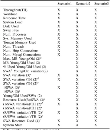
Our approach is based on an experimental approach. We monitor the system and based on the parameters collected the Machine Learning algorithms have to predict the system state (Green, Orange, Red). Table II presents the set of variables used to build every model per scenario: A set of system parameters and a set of derived metrics from parameters. The most relevant of them (derived metrics) is the SWA (sliding window average) of all monitored resources (system parameters) in order to calculate the trend of the resource consumption.

Three different states: Green (all Ok), Orange (Warning) and Red (Danger), have been used for defining the system state. The Red zone is defining when the system is 5 minutes before crash. Orange zone is in the previous 5 minutes to Red zone and the rest is a Green zone.

2) Scenario 1 Description: First scenario evaluates the pre-diction accuracy of the ML algorithms under a deterministic software anomaly. We injected a deterministic and constant memory leaks everyN client visits.

The models have been trained by only 6 failure executions with different workloads (number of clients). The testing data set is obtained after select a subset of instances (20% per each type of instances, green, orange and red). Finally, the selected instances from training and validation data set have been removed.

3) Scenario 2 Description: The second scenario evaluates the models for predicting progressive but dynamic software

(4)

TABLE II

VARIABLES USED IN EVERY EXPERIMENT TO BUILD THE MODELS

Scenario1 Scenario2 Scenario3

Throughput(TH) X X X Workload X X X Response Time X X X System Load X X X Disk Used X X X Swap Free X X X Num. Processes X X X

Sys. Memory Used X X X

Tomcat Memory Used X X X

Num. Threads X X X

Num. Http Connections X X X

Num. Mysql Connections X X X

Max. MB Young/Old (2)a _X _X

MB Young/Old Used (2) X X

% Used Young/Old Used (2) X X

SWAb _{Young/Old variation(2)} _X _X

SWA variation (3)c _X _X _X SWA variation /TH (2)d _X _X _X SWA variation /TH (2)e X X 1/SWA (3)c _X _X _X 1/SWA (3)e _X _X Young/Old Used/SWA (2) X X Resource Used(R)/SWA (3)c _X _X _X (1/SWA variation)/TH (2)d _X _X _X (1/SWA variation)/TH (2)e _X _X (R/SWA variation)/TH (2)d X X X (R/SWA variation)/TH (2)e _X _X

SWA Resource Used (4)f _X _X _X

System State X X X

a_{(X) number of variables represented}

b_{Sliding Window Average (SWA)}

c_{For Num. Threads, Tomcat Mem. Used and System Mem. Used}

d_{For Tomcat Memory Used and System Memory Used}

e_{For Young Zone Used and Old Zone Used}

f_{For Response Time, Throughput, System Memory Used and Tomcat}

Memory Used

anomaly under constant workload. We have trained the model with four previous executions. One hour execution without any memory injection and three executions with memory leak injection (1MB) with different injection ratios: moderate, aggressive and very low. The faulty executions have been run until the crash of the system. This allows the models to learn how the system crashes.

The memory injecting ratio is changed every 20 minutes in the testing scenario: No memory injection, moderated memory injection, aggressive injection and very slow injection rate.

4) Scenario 3 Description: Finally, our last scenario con-siders an aging caused by two resources simultaneously. The two resources involved were memory and threads. The training data set has the same executions from scenario 2 to train the model from memory exhaustion. To learn the threads behavior we have added to the training and validation data set three executions were the resource causing the crash is Threads. We follow the same approach like memory: mod-erate threads injection, aggressive threads injection and very slow threads injection rate. So, the model never was trained using executions where both resources were injecting errors simultaneously. We note that as we are working in a Java

Fig. 1. Resource evolution during Scenario 3 - two resources experiment

environment (Tomcat is a web application running within Java Virtual Machine) Java memory and Java threads are related after all, even on the surface both resources are unrelated; we believe this may be a common situation, and that it may easily go unnoticed even to expert eyes.

The testing data set is an experiment where we changed the injection ratio of both resources every 30 minutes: No injection stage(both resources), a moderate memory injection rate and moderate thread injection rate stage, an aggressive memory rate injection and very slow thread rate injection stage, and finally a very slow memory rate injection and an aggressive thread rate injection. Figure 1 shows the resource behavior during the experiment used to test the best algorithm obtained during validation phase.

B. Training & Validation Experimental Results

This section presents the errors obtained by the Machine Learning algorithms in every scenario using cross-validation process to calculate the prediction error. Due to reasons of space only the best errors obtained by every algorithm are presented. We have tuned every algorithm using thecomplexity parameter available to find the best algorithm and its best configuration. Table III summarizes the results.

ML Algorithms Scenario 1 -Best Error Scenario 2 -Best Error Scenario 3 -Best Error Rpart 1.91% 1.59% 1.23% Naive Bayes 49.66% 32.99% 96.28% SVM-C 4.22% 7.46% 6.12% knn 4.26% 3.67% 3.87% Random Forest 0.63% 0.53% 0.47% LDA 5.43% 4.08% 4.52% QDA 17.61% 4.08% 4.52% TABLE III

VALIDATIONERRORCOMPARISON

We can observe clearly how in all three scenarios Random Forest algorithm obtains a much better error than the rest of the models. According to the model assessment process, we have to select to conduct the testing phase the best of them. In this case we select Random Forest. Random Forest has several parameters to affect the model building process. However, we have conducted the tuning phase playing with only one of them, the most relevant for us: the size of the trees, defined

(5)

Scenario 1 − Predicted vs. Observed System State

Time Instances (15 seconds each)

System State (Green,Or

ange

,Red)

Green

Orange

Red

Observed System State

Green

Orange

Red

100 200 300 400 500 600

Predicted System State

Fig. 2. Scenario 1 - Comparison between observed and predicted system

state

bymtry. In this case, the best configuration of the model varies from one scenario to another:mtry=15,10 and 15 respectively. C. Testing Experimental Results

This section shows the results obtained by best Random Forest models obtained during previous phase.

Predicted State

Observed State

Green Orange Red

Green 655 2 0

Orange 4 19 1

Red 0 1 21

TABLE IV

CONFUSIONMATRIXRANDOMFORESTSCENARIO1

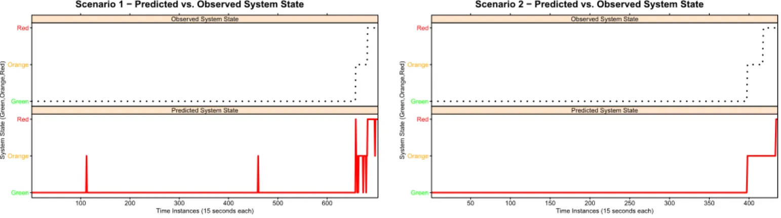
1) Scenario 1: In Scenario 1, the error obtained by the model of Random Forest was 1.13%. At this level of analysis, it is necessary to stablish the type of the errors of the prediction: false positives or negatives. This is relevant because this type of errors may lead to system crashes. A false negative errors could cause an unplanned crash. For this reason, the confusion matrix from Scenario 1 in Table IV has been presented. The diagonal of the confusion matrix represents the right results, where the observed (real) system state is equal to the predicted state. The rest of positions of the matrix represent errors in the prediction. In this scenario, it can be observed how the green, orange and red zones have high prediction accuracy.

At this point need to know where errors are occurring. Figure 2 presents a comparison of the predicted and observed state. It can be observed the four false negatives (green) that are occurring during the orange zone. This is dangerous for the availability of the system because the rejuvenation action has to be trigger during the orange zone to have enough time to finish it.

Although, this prediction is not too bad for applying a proactive rejuvenation action. Because, the model is predicting danger (red), and never backs to green. The rejuvenation action could be triggered in advance. There are two false positive predictions during the green zone. However, this is not dangerous because the rejuvenation action cannot be triggered

ange

,Red)

Green

Orange

Red

Green

Orange

Red

50 100 150 200 250 300 350 400

state

after the first orange prediction. Therefore, it is necessary to wait until the state is confirmed.

2) Scenario 2: The same analysis has been conducted in Scenario 2. The Random Forest model prediction error was 3.67%. Table V presents the confusion matrix of Scenario 2 and Figure 3 shows the comparison of predicted and observed system state in order to analyze in detail where the errors were occured. In this case, it can be clearly observed how the model is able to predict the warning zone. Thus, the prediction model does not generates any dangerous false negative. From availability point of view, an prediction error between orange and red zones is not dangerous because the proactive recovery action would be triggered during the orange zone.

Predicted State

Observed State

Green Orange Red

Green 397 0 0

Orange 0 20 0

Red 0 16 3

TABLE V

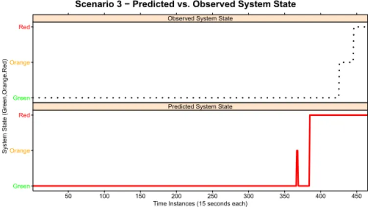
3) Scenario 3: The error obtained by the model generated during Training phase in Scenario 3 was 13.54%. It is observed an increment of the percentage error.

Predicted State

Observed State

Green Orange Red

Green 382 2 41

Orange 0 0 20

Red 0 0 20

TABLE VI

However, if we analyze this error in detail using Table VI and Figure 4, it can be observed again how the prediction model never conducts dangerous false negatives, which could cause unplanned downtime. In Figure 4 can be shown how the model is pessimistic predicting orange zone too early. However, this is better than starting the prediction too late.

(6)

ange

,Red)

Green

Orange

Red

Green

Orange

Red

50 100 150 200 250 300 350 400 450

state

VI. FEATURESELECTION BYLASSOREGULARIZATION

After evaluating the six ML algorithms presented before, we have concluded that Random Forest was the best option. However, to generate the models we were playing with 31 (Scenario 1) and 49 (Scenarios 2 and 3) parameters. In a real environment there are hundreds or thousands of parameters. This fact increases the computational cost of the monitor-ing task and the process of buildmonitor-ing the prediction models. Furthermore, the irrelevant parameters could introduce noise on the models prediction accuracy. For this reason, we have analyzed a sparse regression called Lasso regularization in order to reduce (automatically without human intervention) the number of parameters needed to build the Random Forest Model.

A. Lasso Regularization Details

A machine learning task is equivalent to learning a function or a close approximation to it, given the values of the function at some points [14],[16]. These values will be called training data. There could be many functions, which satisfy the training data or have a small difference. A measure of how well a function matches the training data is the Empirical Risk[15]. Therefore, a function that minimizes the Empirical Risk might look like a good candidate function. However, such functions have the drawback that they overfit the training data i. e., these functions adjust themselves to the training data for the cost of making themselves more complicated, which leads to them having uncontrollable and hard to predict behavior if evaluated at other points. Therefore, many machine learning method try to regularize such functions by assigning some penalty to their complexity i. e., the more complicated the function, the higher is the penalty.

The most common and widely known regularization tech-nique is Tikhonov regularization [22]. It selects the function to be learned by the following rule:

f = arg min f∈H 1 m m X k=1 V(f(Xk), Yk) +λ||f||H (1)

In this formula H is the space of all functions that are considered (usually some Hilbert space with a defined norm,

usually L2 norm),mis the size of the training data,(Xk, Yk)

is the format of the training data -Xkis a vector of parameters

andYk is a scalar or a vector of values that somehow depend

on the parameters (in this paper Yk is the remaining time to

crash),V is a loss function that penalizes empirical errors.λ

is a parameter, which controls how much to regularize and how important is minimizing the empirical risk. Usually, the best value forλis selected through a cross-validation.

Lasso differs slightly from Tikhonov regularization and the difference is that the norm on the function is not given by the Hilbert Space the function is in, but is the L1 norm. The function selection rule takes the form:

f(x) =< β, x > (2)

wherexcan be any vector variable of parameters. The vector

β is derived by: β = arg min β∈Rdim(Xk) 1 m m X k=1 (< β, Xk >−Yk)2+λ||β||L1 (3) The functions that Lasso regularization considers are re-stricted to linear functions but it has the property that the selected weight vector β is sparse, i.e. the majority of its coordinates are zeros.

The Lasso regularization was successfully used in [23] showing it effectiveness to reduce the number of parameters against software anomalies scenario.

B. Training & Validation of Random Forest after Feature Selection by Lasso

In this section, we present the best validation error obtained by Random Forest algorithms for different λ of the Lasso regularization technique. It is worth nothing the validation of random forest algorithm using different values of its com-plexity parametershas been conducted. Table VII summarizes the best validation error obtained. It can be observed clearly how the Lasso regularization allows us to reduce the number of parameters as well as reducing the error in several cases respect to no-Lasso regularization. It is relevant to point out that too much reduction of parameters (even reducing around 90% of parameters) is increasing the validation error. However, it can be considered that a 5% of validation error could be acceptable. Based on the presented results, it can be selected the best λ value for every scenario:0.1, 10000 and 100000, using to build the model only 20, 23, 19 parameters respectively. This means a reduction of parameters up to 35.4%, 53.06% and 61.22% per a scenario.

C. Testing Experimental Results of Random Forest after Fea-ture Selection by Lasso

Results from Scenario 1 are described in Table VIII and Figure 5. In this case, the obtained results are improved compared the results obtained without Lasso regularization. The number of false negatives (earlier 4, now 3) has been reduced. As well, the the number of orange hits (from 19 to 20) is increased, in addition the parameters have been reduce

(7)

Scenario 1 Scenario 2 Scenario 3

λ #Vara _%error _#Vara _%error _#Vara _%error

No Lasso 31 0.74% 49 0.53% 49 0.47% 0.0000001 20 0.63% 33 0.47% 31 0.41% 0.000001 20 0.63% 33 0.47% 31 0.41% 0.001 20 0.63% 33 0.47% 30 0.54% 0.1 20 0.63% 32 0.47% 30 0.54% 1 19 0.74% 32 0.47% 30 0.54% 10 20 0.74% 32 0.47% 30 0.54% 100 20 0.74% 30 0.41% 29 0.44% 1000 18 0.74% 25 0.41% 25 0.44% 10000 17 0.67% 23 0.41% 25 0.41% 100000 15 0.74% 22 0.53% 19 0.26% 1000000 15 0.71% 18 0.47% 19 0.39% 10000000 14 0.88% 6 0.65% 15 0.49% 100000000 12 0.99% 4 2.07% 5 0.65% 1000000000 2 4.36% 4 2.07% 5 0.65% 10000000000 2 4.36% 2 5.21% 3 3.40%

a_{Number of Variables used to build the models}

TABLE VII

VALIDATION ERRORS ACCORDING TOLASSO FEATURE SELECTION

RESULTS

Scenario 1 with Lasso − Predicted vs. Observed System State

ange

,Red)

Green

Orange

Red

Green

Orange

Red

100 200 300 400 500 600

state with Lasso

from 31 to 20. The percentage of testing error obtained in this Testing Scenario is 0.99%.

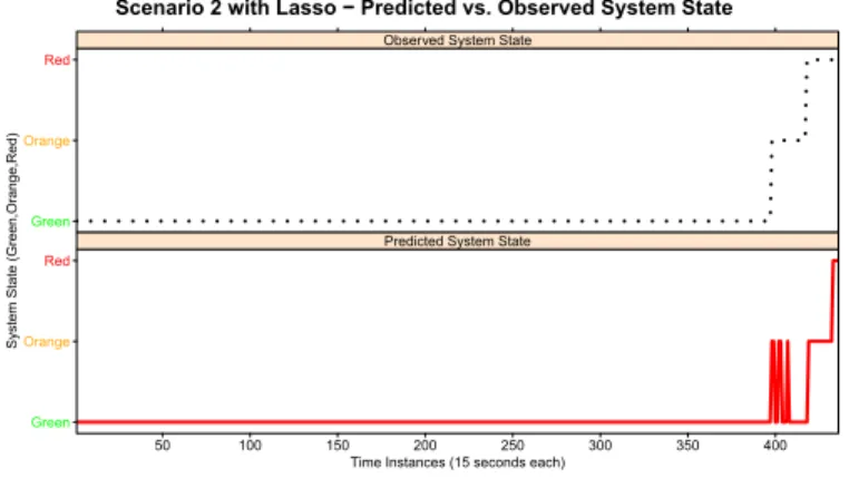
Table IX and Figure 6 summarize the results obtained in Scenario 2. It can be observed how the prediction in the warning zone (orange) is less stable than previously. However, when the system goes inside dangerous (red) zone the model predicts stable warning zone (orange). The percentage of testing error obtained in this Testing Scenario is 6,88%.

Predicted State

Observed State

Green Orange Red

Green 655 2 0

Orange 3 20 1

Red 0 1 21

TABLE VIII

CONFUSIONMATRIXRANDOMFORESTSCENARIO1WITHLASSO

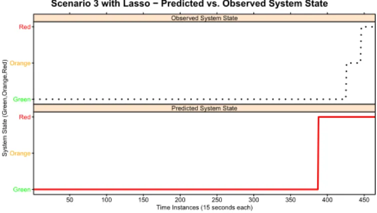
The results of scenario 3 are presented in Table X and Figure 7. The results are relevant because proactively the system will be rejuvenated, when it is in a Green state (38 instances) or in Orange state (20 instances) after, approximately, 380 instances the of the ”perfect prediction” (zero false negatives) i.e.

-Scenario 2 with Lasso − Predicted vs. Observed System State

ange

,Red)

Green

Orange

Red

Green

Orange

Red

50 100 150 200 250 300 350 400

state with Lasso

387 green, Orange 0 and Red 0 instances. In this case ,the system is close to the moment when is ”about to crash”, but based on the ML technique and using Lasso regularization for reducing significantly the number of the monitored parameters will be ”safety rejuvenated”. It can be called ”proactive safe rejuvenation interval”. The percentage of testing error obtained in this Testing Scenario is 12.47%.

Predicted State

Observed State

Green Orange Red

Green 397 0 0

Orange 15 5 0

Red 1 14 4

TABLE IX

VII. RELATEDWORK

Several works investigated the predictions or detection of software anomalies. In [24], authors use time-series ARMA models from the system data to estimate the resource exhaus-tion due to workload received by the system. The aging eval-uated was based on assuming a general trend of the software aging. Moreover, their analysis is based on the knowledge a priorithe resource involved in the aging.

Predicted State

Observed State

Green Orange Red

Green 387 0 38

Orange 0 0 20

Red 0 0 20

TABLE X

In [5], authors conducted a set of analysis to calculate the trend of the aging using a set of different non-parametric statistical methods. After that they used time-series analysis to predict future values of any resource and calculate if the resource will be depleted. They use statistical approaches over known anomaly resources while we use Machine Learning techniques to detect autonomously the software anomalies.

In [25], authors are analyzing of three well-known Machine Learning algorithms: Naive Bayes, Decision Trees and Support

(8)

Scenario 3 with Lasso − Predicted vs. Observed System State

ange

,Red)

Green

Orange

Red

Green

Orange

Red

50 100 150 200 250 300 350 400 450

state with Lasso

Vector Machines to evaluate their effectiveness to model and predict deterministically software anomalies. However, the au-thors did not validate their approach against a dynamic setting or multi-resource exhaustion causing the software anomalies. In [26], the authors present a framework to predict critical events in large-scale clusters. They compare different time-series analysis methods and rule-based classification algo-rithms to evaluate their effectiveness for predicting differ-ent types of critical evdiffer-ents and system metrics. An on-line framework for determining whether a system is suffering an anomaly, a workload change, or a software change is presented [27]. This approach is complementary to the work presented in this paper. The underlying assumption in [27] is that the system admits a static model. The model only depends on the workload and does not degrade or drift over time. However, the analysis and validation of different techniques presented in the current paper are concentrated on the systems that can degrade.

VIII. CONCLUSION

In this paper, a set of ML algorithms has been analyzed for predicting system crashes due to the resource exhaustion caused by software anomalies. Extensive experimental studies, in three different and complex scenarios, have been conducted to show the level of adaptability and prediction accuracy of the ML algorithms. The lowest validation error (less than 1%) in all scenarios has been obtained by Random Forest algorithm. Furthermore, Lasso regularization has analyzed for reducing (up to the 60%) the number of parameters, under monitoring, without paying a penalty in the accuracy prediction.

These results show clearly the effectiveness of Machine Learning techniques for designing monitoring frameworks for improving proactive rejuvenation techniques.

ACKNOWLEDGMENT

This research work has been supported by the Spanish Ministry of Education and Science (projects TIN2007-60625) and by the Generalitat de Catalunya (2009-SGR-980). We also thank to Prof. Jordi Torres and Prof. Ricard Gavald`a for their support and advices during this work.

REFERENCES

[1] Y. Huang, C. Kintala, N. Kolettis, and N. Fulton, “Software rejuvenation: Analysis, module and applications,” inFTCS ’95: Procs. of the 25th Intl. Symp. on Fault-Tolerant Computing, 1995, p. 381.

[2] V. Castelli, R. E. Harper, P. Heidelberger, S. W. Hunter, K. S. Trivedi, K. Vaidyanathan, and W. P. Zeggert, “Proactive management of software aging,”IBM J. Res. Dev., vol. 45, no. 2, pp. 311–332, 2001.

[3] M. J. R. Grottke, M. and K. S. Trivedi, “The fundamentals of software

aging,” in Proc. 1st Intl. Workshop on Software Aging and

Rejuvena-tion/19th IEEE Intl. Symp. on Software Reliability Engineering, 2008. [4] K. J. Cassidy, K. C. Gross, and A. Malekpour, “Advanced pattern

recognition for detection of complex software aging phenomena in

online transaction processing servers,” inDSN ’02: Procs. Intl. Conf.

on Dependable Systems and Networks, 2002, pp. 478–482.

[5] M. Grottke, L. Li, K. Vaidyanathan, and K. S. Trivedi, “Analysis of

software aging in a web server,” IEEE Transactions on Reliability,

vol. 55, pp. 411–420, 2006.

[6] L. M. Silva, J. Alonso, P. Silva, J. Torres, and A. Andrzejak, “Using virtualization to improve software rejuvenation,” in6th IEEE Intl. Symp. on Network Computing and Applications (NCA 2007), 2007.

[7] K. Vaidyanathan and K. Trivedi, “A comprehensive model for software

rejuvenation,”IEEE Trans. Dependable Secur. Comput., vol. 2, no. 2,

pp. 124–137, 2005.

[8] J. Alonso, J. L. Berral, R. Gavald`a, and J. Torres, “Adaptive on-line

software aging prediction based on machine learning,” in Procs. 40th

IEEE/IFIP Intl. Conf. on Dependable Systems and Networks, 2010.

[9] The Comprehensive R Archive Network,CRAN

http://cran.r-project.org/.

[10] J. R. Quinlan,C4.5: programs for machine learning. San Francisco,

CA, USA: Morgan Kaufmann Publishers Inc., 1993.

[11] R. O. Duda, P. E. Hart, and D. G. Stork,Pattern Classification, 2nd ed. New York: Wiley, 2001.

[12] V. N. Vapnik,Statistical Learning Theory. Wiley-Interscience, Sep.

[13] L. Breiman, “Random forests,”Mach. Learn., vol. 45.

[14] T. Poggio and S. Smale, “The mathematics of learning: Dealing with

data,”Notices of the American Mathematical Society, vol. 50, 2003.

[15] O. Bousquet, S. Boucheron, and G. Lugosi, “Introduction to statistical learning theory,” inIn , O. Bousquet, U.v. Luxburg, and G. Rsch (Editors. Springer, 2004, pp. 169–207.

[16] C. M. Bishop,Pattern Recognition and Machine Learning (Information

Science and Statistics). Springer-Verlag New York, Inc., 2006. [17] P. A. Devijver and J. Kittler,Pattern recognition: A statistical approach.

Prentice Hall, 1982.

[18] K. Vaidyanathan and K. S. Trivedi, “A measurement-based model for estimation of resource exhaustion in operational software systems,” in

Procs. 10th Intl. Symp. on Software Reliability Engineering, 1999.

[19] TPC-W Benchmark Java Version,TPC-W

http://www.ece.wisc.edu/ pharm/.

[20] MySQL Data Base Server,MySQL

http://www.mysql.com.

[21] Apache Tomcat,Apache Tomcat

http://tomcat.apache.org/.

[22] F. Cucker and S. Smale, “On the mathematical foundations of learning,”

Bulletin of the American Mathematical Society, vol. 39, pp. 1–49, 2002. [23] D. Simeonov and D. R. Avresky, “Proactive software rejuvenation based on machine learning techniques,” in1st Intl. Symp. on Cloud Computing. ICT, Munich, Germany, October 2009.

[24] L. Li, K. Vaidyanathan, and K. S. Trivedi, “An approach for estimation

of software aging in a web server,” in ISESE ’02: Procs. 2002 Intl.

Symp. on Empirical Software Engineering, 2002, p. 91.

[25] A. Andrzejak and L. Silva, “Using machine learning for non-intrusive

modeling and prediction of software aging,” in IEEE/IFIP Network

Operations & Management Symp., 2008.

[26] R. K. Sahoo, A. J. Oliner, I. Rish, M. Gupta, J. E. Moreira, S. Ma, R. Vilalta, and A. Sivasubramaniam, “Critical event prediction for

proactive management in large-scale computer clusters,” inKDD ’03:

Procs. of the 9th ACM SIGKDD Intl. conf. on Knowledge discovery and data mining, 2003, pp. 426–435.

[27] L. Cherkasova, K. M. Ozonat, N. Mi, J. Symons, and E. Smirni, “Anomaly? application change? or workload change? towards automated

detection of application performance anomaly and change.” inThe 38th

IEEE/IFIP Intl. Conf. on Dependable Systems and Networks. IEEE Computer Society, 2008, pp. 452–461.