Theses 4-27-2020
Deep Convolutional Networks without Learning the Classifier
Deep Convolutional Networks without Learning the Classifier
Layer
Layer
Zhongchao Qian [email protected]
Follow this and additional works at: https://scholarworks.rit.edu/theses Recommended Citation
Recommended Citation
Qian, Zhongchao, "Deep Convolutional Networks without Learning the Classifier Layer" (2020). Thesis. Rochester Institute of Technology. Accessed from
This Thesis is brought to you for free and open access by RIT Scholar Works. It has been accepted for inclusion in Theses by an authorized administrator of RIT Scholar Works. For more information, please contact
Zhongchao Qian
B.Eng. Tianjin University, 2017
A thesis submitted in partial fulfillment of the requirements for the degree of Master of Science in the Chester F. Carlson Center for Imaging Science
College of Science
Rochester Institute of Technology April 27, 2020
Signature of the Author
Accepted by
ROCHESTER, NEW YORK CERTIFICATE OF APPROVAL
M.S. DEGREE THESIS
The M.S. Degree Thesis of Zhongchao Qian has been examined and approved by the
thesis committee as satisfactory for the thesis required for the
M.S. degree in Imaging Science
Dr. Christopher Kanan, Thesis Advisor Date
Dr. Guoyu Lu Date
Dr. Nathan Cahill Date
Submitted to the
Chester F. Carlson Center for Imaging Science in partial fulfillment of the requirements
for the Master of Science Degree at the Rochester Institute of Technology
Abstract
Deep convolutional neural networks (CNNs) are effective and popularly used in a wide variety of computer vision tasks, especially in image classification. Conventionally, they consist of a series of convolutional and pooling layers followed by one or more fully con-nected (FC) layers to produce the final output in image classification tasks. This design descends from traditional image classification machine learning models which use engi-neered feature extractors followed by a classifier, before the widespread application of deep CNNs. While this has been successful, in models trained for classifying datasets with a large number of categories, the fully connected layers often account for a large percentage of the network’s parameters. For applications with memory constraints, such as mobile devices and embedded platforms, this is not ideal. Recently, a family of architectures that involve replacing the learned fully connected output layer with a fixed layer has been proposed as a way to achieve better efficiency. This research examines this idea, extends it further and demonstrates that fixed classifiers offer no additional benefit compared to simply removing the output layer along with its parameters. It also reveals that the typical approach of having a fully connected final output layer is inefficient in terms of parameter
count. This work shows that it is possible to remove the entire fully connected layers thus reducing the model size up to 75% in some scenarios, while only making a small sacrifice in terms of model classification accuracy. In most cases, this method can achieve comparable performance to a traditionally learned fully connected classification output layer on the ImageNet-1K, CIFAR-100, Stanford Cars-196, and Oxford Flowers-102 datasets, while not having a fully connected output layer at all. In addition to comparable performance, the method featured in this research also provides feature visualization of deep CNNs at no additional cost.
port, and guidance, in research work and life. Research is full of challenges and setbacks, and Dr. Kanan helped me overcome a lot of the difficulties. Also my thesis committee who provided suggestions and feedback. My time working at kLab has been pleasant and I would like to thank everyone in the lab. I also appreciate the help from all faculties and staff in the Center for Imaging Science. My friends and family provided a lot of emotional support and help. Finally DARPA who provided funding for the lifelong machine learning project which this work is part of.
1 Introduction and Motivation 1
2 Background work 5
2.1 Alternative Classifiers . . . 5
2.2 Parameter Reduction Techniques . . . 7
2.3 Model Visualization . . . 8
3 Methods 9 3.1 Learned Fully Connected Classifier . . . 9
3.2 Fixed Orthogonal Classifier . . . 11
3.3 Fixed Hadamard Classifier . . . 12
3.4 Fixed Identity Classifier . . . 14
4 Experiments 17 4.1 Architectures . . . 17
4.2 Datasets . . . 19
4.3 Implementation Details . . . 20
4.3.1 General Details . . . 20
4.3.2 Adapting ResNet-32 with the Fixed Identity Classifier on CIFAR-100 22 5 Results 24 5.1 Results on CIFAR-100 . . . 24
5.2 Results on ImageNet-1K . . . 26
5.3 Scalability of fixed classifiers . . . 28
5.4 Fine-Tuning with More Datasets . . . 29
5.5 Feature Visualizations with ResNet-50 . . . 30
5.6 Attempts to improve the method . . . 31
5.6.1 Orthogonal initialization and regularization . . . 32
5.6.2 Alternative pooling methods . . . 33
5.7 Summary . . . 35
6 Discussions 36 6.1 Benefits over other fixed classifiers . . . 37
6.2 Parameter efficiency . . . 37
6.3 Compute efficiency . . . 39
6.4 Summary . . . 40
7 Conclusion 41 Appendices 43 A Source Code (Selection) 44 A.1 Model Architectures . . . 44
A.2 Main Script . . . 62
1.1 Bar plot showing the percentage of parameters in different parts of various deep CNN architectures. . . 3
3.1 A depiction of the fixed identity classifier method. . . 15
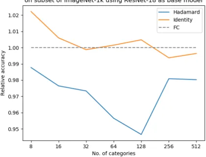
5.1 Relative performance of fixed Hadamard classifier and fixed identity classi-fier, against a learned classifier. . . 30 5.2 Visualizations using fixed identity classifier with the ResNet-50 architecture
fine-tuned on ImageNet-1K. Maximally activated classes are visualized for each object. Normalized scores and class labels are shown in the top-left corner of each visualization. . . 32 5.3 Feature map visualizations for images contain multiple categories from
ImageNet-1K. . . 33 5.4 CNN visualization for original image size (500px × 500px) and resized
(224px ×224px) . . . 34
4.1 CIFAR-100 training hyperparameters settings for each architecture. . . 21 4.2 ImageNet-1K training hyperparameters settings for each architecture. . . . 21 4.3 Transfer learning parameter settings for each architecture. . . 22
5.1 Results on CIFAR with different models and different types of classifiers. . 25 5.2 Results on ResNet-18 with each type of classifier, performing classification
on ImageNet-1K and its subset. . . 27 5.3 Comparison of classification accuracy of the original ShuffleNet v2 and
Mo-bileNet v2 architectures with the fixed identity classifier method applied, trained on the 100 categories subset of ImageNet-1K. . . 27 5.4 Top-1 accuracy results of different classifiers on smaller subsets of
ImageNet-1K, using ResNet-18 as base architecture. . . 29 5.5 Transfer learning performance evaluation of fixed identity classifiers on
Cars-196 and Flowers-102 using multiple deep CNN architectures. . . 31 5.6 Top-1 accuracy results of different orthogonal initialization and
regulariza-tion configuraregulariza-tions, using ResNet-18 as base on ImageNet-1K 100 category subset. . . 34
6.1 Compute cost for different components in different architecture in FLOPs, and percentage of compute the final fully connected classifier accounts for. . 39
Introduction and Motivation
The strong performance of deep convolutional neural networks (CNNs) has enabled an enormous number of new computer vision applications. However, many state-of-the-art CNN architectures are ill-suited for deployment on mobile and embedded devices due to their high computational and memory requirements. The vast majority of CNN ar-chitectures are designed as having a feature extractor followed by a classifier. The fea-ture extractor consists of convolutional layers and pooling operations, while the classifier is made up of one or more fully connected layers. This has been a common practice since the early days of deep CNNs, and it descends from traditional image classification methods. In the years before the first deep CNN won the ImageNet Large-Scale Visual Recognition Challenge (ILSVRC) challenge, winning methods as documented in [23, 30] used crafted feature extractors, followed by classifiers based on support-vector machines (SVM). In ILSVRC2012, the winning method AlexNet proposed in [18] is a deep convo-lutional neural network, which has a feature extractor, followed by a classifier using three fully connected layers with ReLU activation in between. In the years followed, popular
architectures, for example the VGG family proposed in [34], all used multiple fully con-nected layers. The first work to change that is Network in Network proposed in [22], it uses a global average pooling (GAP) layer after the feature extractors, and only has a single fully connected layer for the classifier. In [37], GoogLeNet (Inception v1) uses this method and won ILSVRC2014. Since then, using global average pooling followed by a single fully connected layer has been the popular method of implementing the classifier.
A number of papers have developed methods for reducing the parameters in the feature extractor, for instance, in [18], AlexNet first implemented group convolutions, in depth-wise separable convolutions introduced in Xception from [4], and squeeze and expand operations from SqueezeNet presented in [13], but little work has been done to reduce the parameters in the classifier’s fully connected layers. Because the number of parameters in the classifier is typically proportional to the number of categories, the classifier can consume a large portion of the network’s total parameters for large datasets. For example, in MobileNet v2 from [32], the fully connected layers consume 37% of the parameters in the CNN for ImageNet-1K classification.
A few existing works have studied how to reduce the number of parameters in a CNN’s classifier for many-class datasets by using fixed output matrices [10, 29]. These methods initialize the weights, but do not update them during training, thus increasing the efficiency of models.
In this research, this idea is taken further. A fixed identity matrix is used as the classifier, which is equivalent to removing the classifier layer rather than having a fea-ture extractor followed by a classifier. The convolutional layers are trained directly for classification and the traditional classification layer is entirely eliminated. This research shows that the number of parameters can be greatly reduced by rethinking the
architec-ture design, as demonstrated in the bar plots for different architecarchitec-tures for ImageNet-1K classification in Figure 1.1. The green plot shows the total number of parameters for each architecture. As models get more efficient and compact, the final classifier accounts for more of the total parameters. The method presented in this work eliminates the need for a final fully connected (FC) layer for classification, significantly reducing memory require-ments, especially in already efficient models.
ResNet-50 DenseNet-121 MobileNet v2 ShuffleNet v2 x0.5
Parameters in different layers
0 20 40 60 80 100Percentage of total parameters
Classifier Feature Extractor 5 10 15 20 25
Total parameters (in millions)
8% 13%
37%
75%
Figure 1.1: Bar plot showing the percentage of parameters in different parts of various deep CNN architectures.
This research features the following contributions: 1) It shows that the final convolu-tional layer can be modified in many widely used CNN architectures to enable the fully connected layer to be completely eliminated, with little loss in classification performance but with a large reduction in the total number of parameters for many-class datasets. 2) It compares the method against existing fixed classifier methods and achieve superior results,
while being much simpler and more efficient. 3) It shows that the final classifier layer con-tributes little to overall model classification accuracy. Thus suggesting that using a fully connected layer is very inefficient and should be changed in future architecture designs for image classification. 4) It demonstrates that the method’s final convolutional layers are interpretable without needing any additional computation or post-processing, which can be prohibitive on edge devices. This enables the CNN to be used for detection and localization without explicitly using techniques such as Class Activation Mapping (CAM), which was demonstrated in [41].
Background work
This work relates to three main categories of existing work: 1) Alternative classifiers which have been explored mainly for making the output layer more discriminative, or attempting to make the classifier more efficient, 2) Parameter reduction techniques which range from the ground-up redesign of networks to post-trained pruning techniques, and3) Model visualizationwhich are other techniques to provide visual interpretations to deep CNN models. These background work are discussed in detail in the following sections.
2.1
Alternative Classifiers
In [35], a study was conducted to understand what components of a CNN are absolutely necessary. They concluded that a CNN can be constructed using only convolution oper-ations by demonstrating that the final fully connected output layer could be replaced by 1-by-1 point-wise convolutions; however, they did not consider that the entire classification
layer could be removed.
A few existing works have studied how to reduce the number of parameters in a CNN’s classifier for many-class datasets by using fixed output matrices [10, 29]. In [10], it was shown that any fixed orthogonal output matrix could be used to replace a learned output matrix with no reduction in performance. While this does not reduce the number of parameters or computational requirements, they then demonstrated that a Hadamard matrix could be used. A Hadamard matrix can be deterministically generated and does not need to be stored, thus enabling increased efficiency. However, it is not possible to construct a Hadamard matrix if the input to the classifier has fewer dimensions than the number of output categories because a Hadamard matrix’s rows and columns are mutually orthogonal. This means for ResNet-18, which has 512-dimensional features input to the classifier, it would be limited to classifying at most 512 categories. This limitation was overcome in [29], which proposed a different method of creating a fixed output classifier. Their approach uses coordinate values of high-dimensional regular polytopes as rows of the fixed classifier weight matrix. While this approach works, it can be difficult to train, and it is used mainly to optimize for feature extraction.
It is not currently clear which fixed output matrix approach is best, and some of these methods still require the classifier’s parameters to be stored, even if the parameters are not updated during training. In contrast, the approach in this research avoids using an explicit classification layer entirely, eliminating the problem of selecting and storing a fixed classifier weight matrix.
2.2
Parameter Reduction Techniques
A class of popular methods for reducing the number of parameters in the feature extractor is by using variants of convolution operations. Popular techniques include group convo-lutions, depth-wise convoconvo-lutions, bottleneck modules, etc. Group convolutions split the convolution input and output channels into groups, where each group is a convolution operation independent of other groups [18]. By removing connections between channels belonging in different groups, it reduces parameters in the convolution by a factor equal to the number of channels. Depth-wise separable convolution is a two-step procedure. First, there is a group convolution where the number of input channels, output channels, and groups are all the same, followed by a point-wise convolution with the desired number of output channels [4]. In [9], bottleneck modules which has three layers of 1x1, 3x3, and 1x1 convolutions, using the point-wise convolutions to decrease and then increase the dimen-sions, reducing the parameters in the 3x3 convolution. Similar techniques are used in [13], the Fire module uses point-wise convolution to compress the number of channels first, then uses both 3x3 and 1x1 convolutions to expand to the desired number of channels.
Other methods for reducing the number of parameters are pruning and quantization. Pruning removes (zeros out) weights after training to promote sparsity, and a wide variety of pruning methods have been explored [1, 7, 11, 20, 21, 24, 36]. Quantization methods typ-ically reduce the numeric precision of the weights after training, which can greatly reduce the number of parameters [5,14,15]. Both pruning and quantization are complementary to the method proposed in this research, which focuses on eliminating the classifier to reduce the number of parameters.
2.3
Model Visualization
One of the major complaints about CNNs is that they lack interpretability, leading to tools such as CAM [41], Grad-CAM [33], and Grad-CAM++ [3] being developed to better understand the features that led to the output of the classifier. These methods require additional post-processing computation after the model has been run to visualize the evidence used by the classifier to generate its output. In contrast, the approach in this research enables the CNN to be interpreted immediately, without any extra compute required.
Visualization of CNN model is already present when Le Cun developed LeNet-5 for handwritten digit recognition [19], showing the activations in each layer of the network. In [39], Zeiler introduced a method that visualizes intermediate feature layers in deep con-volutional neural networks, giving some insight to the inner workings of deep concon-volutional neural networks.
Inverting the network is another technique that also provides insight to the network itself, and reveals that deep features contain information to reconstruct the input image [6, 26].
Zhou et al. discovered that a deep CNN for image classification can also be used for object detection [40], in the same forward pass calculation. Later they proposed class activation map [41] (CAM), the technique was introduced as a way to visualize which portion of the image a CNN used to make a prediction. It requires using global average pooling in models, and needs extra calculations to produce the CAM. The method in this work can output CAM, during the inference stage in a single forward pass as well, but can do it directly without any other additional calculations.
Methods
In this research, four methods for implementing the classifier are evaluated: 1. using a learned fully connected classifier 2. using a fixed orthogonal projection; 3. using a fixed Hadamard projection; and 4. removing the fully connected layer, which is equivalent to using a fixed identity matrix for projection and setting the bias term to zero. First, the conventional method of using a fully connected classifier will be explained. Then the two fixed projection methods [10] will also be explained. Finally the classifier implementation featured in this work will be demonstrated. All three fixed classifiers will be compared against a learned fully connected classifier, and against each other, to evaluate their effects on the model.
3.1
Learned Fully Connected Classifier
In typical deep neural networks for single-class image classification, the last layer is a fully connected layer of affine transformation, and all its parameters are learned.
First, a few variables will be defined:
• Letf(·) be the feature extractor.
• Letc(·) be the classifier.
• Letx∈R3×h×w be the input to the model, assuming the input is an 3 color channel
RGB image andh,wis its height and width.
• Letncbe the number of output channels from the feature extractor.
• Letfh and fw be the height and width of the output from the feature extractor.
• Letf ∈Rnc×fh×fw be the output feature map,f =f(x).
• Letnk be the number of output categories.
• Leth and hi be intermediate results between layers in the classifierc(·).
• Lety∈Rnk be the output of the model,y=c(h).
In earlier deep convolutional neural networks, for convenience we will use the AlexNet architecture proposed in [18] as an example, f ∈ R256×6×6 is the result of a non-global max pooling operation of kernel size 3×3 in the end of its feature extractor f(·). This feature map f is then flattened into a vector h0 ∈ R9,216. Then it goes through multiple affine transformations followed by non-linear activations, to finally produce the output y∈R1000 as shown in Equation 3.1 below
h1 = ReLU (W1h0+b1)
h2 = ReLU (W2h1+b2)
y= softmax (W3h2+b3).
In the case of AlexNet, the weights for the affine transformations are W1 ∈R4,096×9,216, W2 ∈R4,096×4,096, W3 ∈R1,000×4,096; the biasesb1...3 are of dimensions 4096, 4096, and 1024 respectively. The final non-linear activation is softmax(·), in order to produce the final output, which is the classification likelihood for each potential category.
In more recent architectures, the classifier is a single affine transformation, and its input is produced from a global average pooling (GAP) operation:
h= 1 fh×fw X fh X fw f. (3.2)
By averaging the elements in each channel, we are able to obtainh∈Rnc as the input to the affine transformation and obtain the output:
y= softmax (Wh+b). (3.3)
It is intuitive thatW ∈Rnk×nc andb∈
Rnk. Through the use of GAP, the classifier is still
able to use information from the entire feature map, while consuming way less parameters. In either case, the weight matricesWand biasesbare optimized during back-propagation using gradient descent.
3.2
Fixed Orthogonal Classifier
In a fixed orthogonal classifier [10], everything is the same as using a learned fully con-nected classifier, except for the weight matrix W, which is initialized using a specific matrix, and during back-propagation, it is not updated.
orthogonal matrix is defined as a square matrix Q, where QQT =QTQ=I, and I is an identity matrix. In the case of a semi-orthogonal matrix, the matrix is no longer square. A matrix W is semi-orthogonal if eitherWTW=I orWWT =I.
Given the semi-orthogonality, in the case of nc ≥ nk, the rows of the weight matrix
W are mutually orthogonal; in the case ofnc< nk the columns are mutually orthogonal,
but the rows are not.
In fixed orthogonal classifiers, the weight matrix is not updated during training and is semi-orthogonal, hence its name.
3.3
Fixed Hadamard Classifier
In fixed Hadamard classifiers [10], the weight matrix is also fixed (i.e., not updated), and it is initialized from a Hadamard matrix. In this case, the Hadamard matrix is constructed using Sylvester’s construction. Let H1 be a Hadamard matrix of order 1, defined as
H1 =
1
. (3.4)
Let k be any non-negative integer greater than 1. Higher order Hadamard matrices of order 2k can be constructed using Hadamard matrices of the lower order 2k−1, given as,
H2k = H2k−1 H2k−1 H2k−1 −H2k−1 . (3.5)
By iterating this process, we can obtain Hadamard matrices of order 1, 2, 4, . . . , 2k. To construct the weight matrix, we would need to obtain a Hadamard matrix of order
2k, wherek=dlog2max(nc, nk)e. Then the matrix is truncated to fit the size of the input
and output, by taking its firstnc rows and firstnk columns.
For instance, if we have 3 output channels from the feature extractorf(·), i.e. nc= 3,
and we have 2 output categories, i.e. nk = 2 then we know the input to the classifier
h∈R3 and the desired output isy∈R2. To construct the weight matrix we can calculate
k=dlog2max(3,2)e=dlog23e= 2, therefore we need to construct a Hadamard matrix of order 22= 4.
Using Sylvester’s construction, we have
H1 = 1 , H2 = 1 1 1 −1 , and finally H4 = 1 1 1 1 1 −1 1 −1 1 1 −1 −1 1 −1 −1 1 .
Then we can truncateH4 to obtain
W= 1 1 1 1 −1 1 .
Then the output is obtained using the following calculation:
y=αWh+b , (3.6)
whereα is a learned scalar parameter that is updated during back-propagation and h is the input to the classifier.
The fixed Hadamard classifier using this construction has a limitation. It cannot produce effective outputs when the output dimension is larger than that of the input. For instance when using it in ResNet-18 for classification of ImageNet-1K, the input is a vector of 512 dimensions, while the output needs to be 1000 dimensions. HereW has 1000 rows and 512 columns, and it is apparent that rows 513 through 1000 are identical to rows 1 through 488, resulting in the same intermediate results for all these items. The final results only differ becauseb could be different. This is also very apparent from observing the first two columns ofH4 constructed earlier, the first two elements from rows 1 and 3, or rows 2 and 4, are the same.
3.4
Fixed Identity Classifier
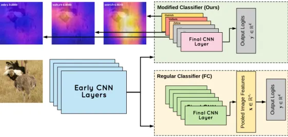
This is the method featured in this work. Here, the final fully connected layer is com-pletely removed, and the output from the global average pooling layer is directly used to compute classification scores. The global average pooling layer is immediately after the last convolution layer in the feature extractor. By removing the FC layer, it greatly reduces the number of parameters in the network. A depiction of this method is shown in Figure 3.1. Implementation wise, it is equivalent to setting the weight matrix W as an identity matrix I, where all the elements on the diagonal are 1 and all other elements
are 0. This matrix is not updated throughout training. The bias term,b, is also dropped. Regular Classifier (FC) P o o le d I m a g e F e a tu re s O u tp u t L o g it s Final CNN La yer Ostrich Final CNN La yer Vulture Final CNN La yer Zebra Final CNN La yer ... Final CNN La yer ... Final CNN La yer Final CNN La yer Final CNN La yer Final CNN La yer Final CNN La yer Final CNN La yer Final CNN La yer Ear ly CNN La yer s Ear ly CNN La yer s Ear ly CNN La yer s Ear ly CNN La yer s O u tp u t L o g it s
Modified Classifier (Ours)
Figure 3.1: A depiction of the fixed identity classifier method.
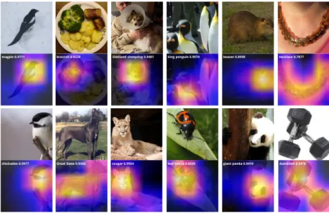
This method offers an additional benefit: since each channel in the output of the final CNN layer represents an output class, it enables the outputs to be visualized immediately, similar to class activation mappings (CAM) [41]. Contrary to CAM which requires post-processing intermediate results from the neural network, this method can obtain these visualizations without any extra compute, during the forward pass (inference), along with obtaining the classification scores. The visualization results are demonstrated in Fig-ure 3.1, using an image of ostrich from ImageNet-1K test set. As shown in the figFig-ure, they can be directly visualized to represent class-specific visualizations. The model produces high activation for regions with the correct class (ostrich), low activation for an unrelated class (zebra), and regions containing background objects (vulture).
This method suffers the same limitation as a fixed Hadamard classifier: it is unable to handle cases where the number of classification categories is greater than the number
of channels from the last convolution layer. However, this research is not promoting the method as a drop-in replacement on existing architectures, it serves as a proxy tool to study the final classifier layer in current image classification architectures, and a possible method to design classifiers for future efficient architectures.
Experiments
To demonstrate the effectiveness of fixed identity classifiers, the methods are evaluated across a variety of base architectures and datasets. All experiments are implemented using the Python programming language on PyTorch, an open-source machine learning framework.
4.1
Architectures
Several common residual networks, as well as mobile architectures that contain far fewer parameters, are chosen as the base architectures:
• ResNet-18– The ResNet-18 architecture is a common residual network consisting of 18 layers and skip connections to help gradient flow [9]. This architecture is used since it is the fastest residual network to train for ImageNet-1K classification.
• ResNet-50– ResNet-50 is a residual network with 50 layers and skip connections [9]. This architecture is chosen since it has been commonly used for computer vision
applications and achieves higher performance on ImageNet than ResNet-18.
• ResNet-32– This variant of ResNet is one variant that is optimized for the CIFAR image classification dataset, where the input image size differs from that used in ResNet-18 and ResNet-50.
• DenseNet– The Dense Convolutional Network takes the skip connection idea fur-ther [12]. In DenseNets, each layer has a skip connection to every ofur-ther layer in a feed forward fashion. In this research, DenseNet-BC (L = 100, k = 12) is used to match the work in [10].
• MobileNet v2– MobileNet architectures are designed to efficiently run on mobile devices by replacing convolutional layers with depth-wise separable convolutions. The MobileNet v2 architecture [32] is used, which additionally uses bottlenecks and residual connections. This architecture is chosen since it is computationally effi-cient and using a fixed identity classifier can further reduce the network’s memory requirements.
• ShuffleNet v2 x0.5 – ShuffleNet architectures use point-wise group convolutions and bottleneck layers to run efficiently on mobile devices. A channel shuffle operation is applied on top of these operations to allow gradients to flow between different channel groups, which improves accuracy. ShuffleNet v2 additionally introduces a channel split operation [25]. In this research, ShuffleNet v2 with half-width (x0.5) is used.
For learned fully connected classifiers, the reference PyTorch implementations from the
torchvisionpackage are used when available, or implemented as described in the original work when the reference implementation is not available. For fixed Hadamard classifiers, the implementation is based on reference code and the source code provided in [10]. For
fixed orthogonal classifiers, the reference implementation with FC is used, but the weights are initialized as a semi-orthogonal matrix and updates for the weight matrix is disabled, which is similar to the implementation in [10]. The fixed identity version simply removes the classifier, and truncates the output to the desired number of dimensions.
4.2
Datasets
Experiments are done on CIFAR-100 to quickly evaluate the performance of fixed identity classifiers. Then, experiments are performed on the ImageNet-1K dataset, demonstrating the robustness of the method on a large dataset with many categories. Additionally, experiments are performed on two smaller datasets to demonstrate the method’s ability to perform transfer learning.
These datasets were chosen because they have a large number of classes, making it possible to test the method’s capability of performing well, while also saving memory. The following datasets are chosen:
• ImageNet-1K – The ImageNet dataset consists of images from 1,000 categories from the internet [31]. Each category consists of 732-1,300 training examples and 50 validation examples, which are used for testing. This is a common large-scale image classification dataset that allows us to test the ability of the fixed identity classifier method to scale up and showcase its parameter savings.
• CIFAR-100 – The CIFAR-100 dataset contains 100 classes each containing 600 color images of size 32×32 [17]. For each class, there are 500 images for training and 100 for testing.
8,144 training and 8,041 testing images [16].
• Flowers-102 – The Oxford Flowers dataset consists of 102 flower categories, with each class containing 40-258 images [27].
While CIFAR allows for a quick evaluation of different methods, ImageNet tests the ability of the method to scale up to a large number of categories. The Stanford Cars-196 and Flowers-102 datasets are used for evaluating the method’s ability to perform fine-grained transfer learning tasks.
4.3
Implementation Details
4.3.1 General Details
PyTorch is used for all experiments. For CIFAR-100, every model on every architecture is trained from scratch. For the ImageNet results using a standard fully connected classi-fication layer, the accuracy from the PyTorch pre-trained models are reported. For other classifiers on ImageNet, the models are trained from scratch. For all other experiments, each model is first initialized with pre-trained ImageNet weights and then fine-tuned on the target dataset.
For training on ImageNet and CIFAR-100, the original setups including methods for data augmentation [9,10,12] are used. For instance, for training ResNet-32 and DenseNet-BC on CIFAR-100, the following data augmentations are performed for training: 4 pixels are padded on each side, then a mirroring is applied at random, followed by cropping to 32×
32 randomly. For testing, the original image is used, only normalization is applied. This follows the practice in their respective work. The specific hyperparameters for training the models are given in Table 4.1, both architectures use the stochastic gradient descent
(SGD) optimizer.
Table 4.1: CIFAR-100 training hyperparameters settings for each architecture.
Hyperparameter ResNet-32 DenseNet-BC
Initial Learning Rate 0.1 0.1
Momentum 0.9 0.9 LR Decay Factor 10 10 LR Decay Epochs [81, 122] [150, 225] Weight Decay 1.0×10⁻⁴ 1.0×10⁻⁴ Batch Size 128 64 Total Epochs 164 300
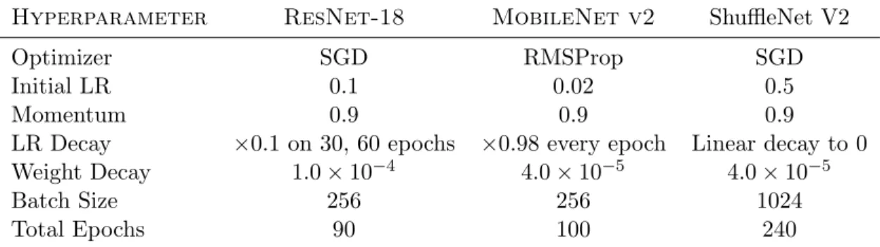
For training on ImageNet, hyperparameters are given in Table 4.2. Note that Mo-bileNet v2 uses the RMSProp optimizer. The training scheme for ResNet-18 and Shuf-fleNet V2 can be found in their original work [9, 25]. As for MobileNet V2, the training scheme is partially described in the original work [32], while also making a reference to to [38].
Table 4.2: ImageNet-1K training hyperparameters settings for each architecture.
Hyperparameter ResNet-18 MobileNet v2 ShuffleNet V2
Optimizer SGD RMSProp SGD
Initial LR 0.1 0.02 0.5
Momentum 0.9 0.9 0.9
LR Decay ×0.1 on 30, 60 epochs ×0.98 every epoch Linear decay to 0 Weight Decay 1.0×10⁻⁴ 4.0×10⁻⁵ 4.0×10⁻⁵
Batch Size 256 256 1024
Total Epochs 90 100 240
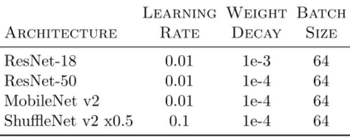
provided in Table 4.3. All networks were trained with stochastic gradient descent and momentum of 0.9 for 40 epochs, with a learning rate decay by a factor of 10 at 30 epochs. Optimal parameters were chosen using a grid search.
Table 4.3: Transfer learning parameter settings for each architecture.
Learning Weight Batch
Architecture Rate Decay Size
ResNet-18 0.01 1e-3 64
ResNet-50 0.01 1e-4 64
MobileNet v2 0.01 1e-4 64
ShuffleNet v2 x0.5 0.1 1e-4 64
4.3.2 Adapting ResNet-32 with the Fixed Identity Classifier on CIFAR-100
Despite the that the fixed identity classifier cannot work with architecture and dataset combination that has more classification categories than the dimensions of the feature vector, a slightly modified version of ResNet-32 is used to compare the effects of using a fixed identity classifier with the architecture to classify CIFAR-100.
The key idea is to modify the last convolution layer to output 100 channels instead of 64 channels. In convolutional networks that appeared before residual networks, this is very easy to implement. However, in ResNets, the network consists of major ”layers” (not individual layers), and each layer has several blocks. Within each block, there are several convolution and pooling operations, and in addition, there is a skip connection between the input and output in every block of the network. This means that the input
to each block goes through an optional transformation and is added to the output from the final convolution layer in each block, skipping the other operations in between, and then this is used as the final output of the entire block. Therefore, simply modifying the last convolution layer will break the network.
There are several ways to implement the skip connection. Identity, zero-padding, and learned projection. In the case of identity, the input is added as-is, this mode can only be used when the number of input and output channels are the same. A learned projection is a learned one-by-one pointwise convolution filter so that the output can be of a different number of channels. Zero-padding means additional channels are created, but the values are all zero.
The original ResNet research showed that using projections in all skip connections is marginally better than using projections only when doubling the channels. And using identity and projection is slightly better than using identity and zero-padding.
To accommodate the modification of the last channel, several methods were explored in preliminary experiments. The results reported uses the zero-padding method as no method is particularly advantageous while zero-padding introduces the least number of new parameters.
Results
All variants of the final classifiers are evaluated on multiple architectures and multiple datasets, to compare and demonstrate their ability to perform image classification. The learned classifier is used as the baseline. To see how much accuracy each classifier is sacrificing, the corresponding top-1 classification accuracy is compared against the baseline results.
5.1
Results on CIFAR-100
DenseNet-BC and ResNet-32 are trained to perform classification on CIFAR-100, while different methods are applied to implement its classifier. The results are shown in Ta-ble 5.1. For DenseNet-BC, all variants of the classifier are used; for ResNet-32, the fixed identity classifier is not used. This is because the fixed identity classifier is incapable of dealing with the feature extractor in ResNet-32, which outputs 64 channels, for 100 cat-egories classification. However, ResNet-32 is trained with the fixed Hadamard classifier,
nk Architecture Classifier Top-1 Accuracy Performance Gap 100 ResNet-32 Learned 69.46% N/A Fixed Orthogonal 68.61% -0.85% Fixed Hadamard 44.86% -24.60%
ResNet-32 w/ Learned 70.23% N/A
100 ch. output Fixed Identity 69.98% -0.25%
DenseNet-BC Learned 77.61% N/A Fixed Orthogonal 76.68% -0.93% Fixed Hadamard 75.84% -1.77% Fixed Identity 76.90% -0.71% 64 ResNet-32 Learned 73.94% N/A Fixed Orthogonal 73.92% -0.02% Fixed Hadamard 73.97% +0.03% Fixed Identity 74.25% +0.31%
even though it is projected that it will not perform well.
A modified version of ResNet-32 as described in Section 4.3.2 is used to compare both a learned classifier and a fixed identity classifier on the same base architecture for the full CIFAR-100 dataset.
To evaluate all the classifiers on a vanilla version of ResNet-32 and CIFAR-100, a 64 categories subset of CIFAR-100 was used so that the number of categories does not exceed the number of output channels from the feature extractor.
This research was unable to reproduce results for DenseNet-BC using the fixed Hadamard classifier, using their original open-source code. In their original work, they report 77.67% for the test accuracy, only 75.84% was achieved in this work. However, the training setup used in this research is fair to all classifiers, therefore the performance gap still shows that
not having a dedicated output layer is slightly superior to using a fixed Hadamard matrix, but not as good as having a learned fully connected classifier.
The results in Table 5.1 indicate that neither the fixed orthogonal classifier nor the fixed Hadamard classifier performs better than the fixed identity classifier, while being more complicated, while exhibiting the same weakness of not capable of working with feature extractors producing less channels than the desired number of classification categories.
In the experiments on the modified ResNet-32, although total parameter count did increase, the comparison between the two classifier methods is still fair. Multiple runs of the experiment was completed for both classifiers, and there was no statistical difference between the classification accuracy from the two methods, although the average for the learned classifier is still higher.
5.2
Results on ImageNet-1K
Moving on to a more challenging dataset, ResNet-18 with different classifiers are trained and evaluated on ImageNet-1K.
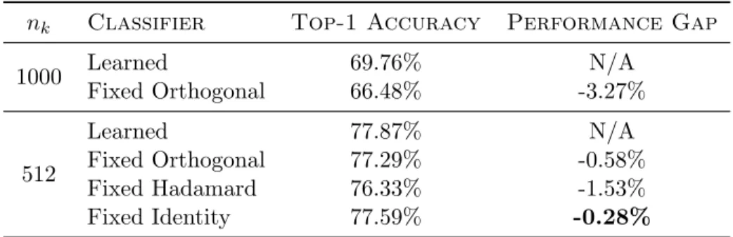
Similar to the situation before, due to limitations of the fixed Hadamard classifier and fixed identity classifier, the full 1000 categories are evaluated only on the learned classifier and the fixed orthogonal classifier. Then all classifiers are evaluated on the first 512 categories of ImageNet-1K, so that the Hadamard classifier and the fixed identity classifier can be compared. The results are shown in Table 5.2. The results indicate that while all fixed weights perform worse than learned weights, using a fixed identity matrix, which is equivalent to removing the classifier layer, outperforms both fixed orthogonal classifiers and fixed Hadamard classifiers.
nk Classifier Top-1 Accuracy Performance Gap 1000 Learned 69.76% N/A Fixed Orthogonal 66.48% -3.27% 512 Learned 77.87% N/A Fixed Orthogonal 77.29% -0.58% Fixed Hadamard 76.33% -1.53% Fixed Identity 77.59% -0.28%
Next, the fixed identity classifiers are used on the mobile architectures, MobileNet v2 and ShuffleNet V2, which are already very compact. Here, only the learned fully connected classifiers are being compared against, as it has been demonstrated that fixed Hadamard classifiers do not perform better. The results can be found in Table 5.3.
Table 5.3: Comparison of classification accuracy of the original ShuffleNet v2 and Mo-bileNet v2 architectures with the fixed identity classifier method applied, trained on the 100 categories subset of ImageNet-1K.
K Architecture Classifier Top-1 Acc.
1000 ShuffleNet V2 x0.5 Learned 60.55% Fixed Identity 53.06% MobileNet v2 Learned 71.88% Fixed Identity 71.03% 100 ShuffleNet V2 x0.5 Learned 72.94% Fixed Identity 74.42%
Shuf-fleNet V2 x0.5 the savings is about 75%, and on MobileNet v2 it’s about 37%. It is apparent that there is a non-trivial degradation in performance in the case of ShuffleNet V2. To evaluate whether this is due to the lack of parameters, or the modification to the architecture, the same tests are run on a very small subset of ImageNet, consisting of only 100 categories, and the results are also shown in Table 5.3. In this case, the fixed identity classifier does not perform worse than a learned classifier. Therefore the major performance gap on ImageNet-1K is likely due to the model being too small rather than the difference in the model architecture.
5.3
Scalability of fixed classifiers
Originally, the study of fixed classifiers, especially fixed Hadamard classifiers, was intended to find a classifier that is capable of scaling to more categories without using as many parameters.
It was quickly determined that a fixed Hadamard classifier does not scale past its input channels. Research is conducted on smaller subsets of ImageNet-1K to compare if a fixed Hadamard classifier performs better in any other case. ResNet-18 with different classifiers are trained on subsets of different sizes, the average top-1 accuracy over three runs are reported in Table 5.4.
The results fluctuate somewhat at different subset sizes, although the variance between three runs that only differ in random seeds is not very big. The fluctuations may be due to overfitting and/or the characteristics of specific categories. The relative performance plot is shown in Figure 5.1, and it is obvious that the fixed identity classifier is better than the fixed Hadamard classifier regardless of how the model scales.
nk Learned Fixed Hadamard Fixed Identity 8 74.92% 74.00% 76.58% 16 83.21% 81.25% 83.71% 32 83.64% 81.38% 83.50% 64 75.51% 72.23% 75.63% 128 77.98% 73.82% 78.36% 256 79.03% 77.52% 78.54% 512 77.87% 76.33% 77.59%
5.4
Fine-Tuning with More Datasets
One issue with removing the classifier (replacing it with an identity matrix) is that it may harm the model’s ability to perform transfer learning. This research demonstrates that the fixed identity classifier can be applied to more datasets and architectures, in transfer learning settings. Results with several architectures on the Stanford Cars-196 and Flowers-102 datasets are shown in Table 5.5, they reflect the average top-1 accuracy of three runs. The results are obtained by fine-tuning a model pretrained on ImageNet.
As the results indicate, the method works on ResNet-18, ResNet-50, MobileNet v2, and ShuffleNet v2 x0.5 on both datasets. It shows that fixed identity classifiers are able to achieve comparable results while using significantly fewer parameters, demonstrating its capabilities in transfer learning and generalization on more datasets.
Figure 5.1: Relative performance of fixed Hadamard classifier and fixed identity classifier, against a learned classifier.
5.5
Feature Visualizations with ResNet-50
Visualizations of the final convolutional layer’s outputs for ResNet-50 trained on ImageNet-1K are given in Figure 5.2. Unlike CAM, by using a fixed identity classifier, no additional post-processing is required to obtain class-specific visualizations.
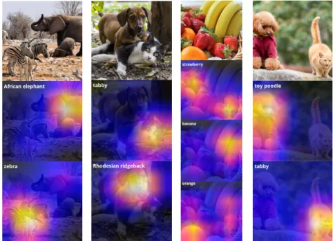
Furthermore, despite being trained with only a single label per image, visualizing the final convolutional layer gives class-specific localization from a single forward pass. In Figure 5.3, several example images that were downloaded from the Internet are shown. They consist of multiple ImageNet-1K object categories, demonstrating that this method is able to produce object localization for free. By selecting multiple channels, this method can easily visualize activation maps for multiple categories. This is similar to the result
Stanford Cars-196
Learned Fixed Identity Savings
ResNet-18 88.12% 86.06% 12.92%
ResNet-50 89.90% 90.35% 5.66%
MobileNet v2 87.68% 86.12% 24.26%
ShuffleNet V2 x0.5 77.99% 75.76% 66.65% Flowers-102
Learned Fixed Identity Savings
ResNet-18 93.42% 92.78% 16.83%
ResNet-50 95.06% 94.64% 5.10%
MobileNet v2. 94.24% 93.95% 21.66%
ShuffleNet V2 x0.5 87.75% 86.34% 63.52%
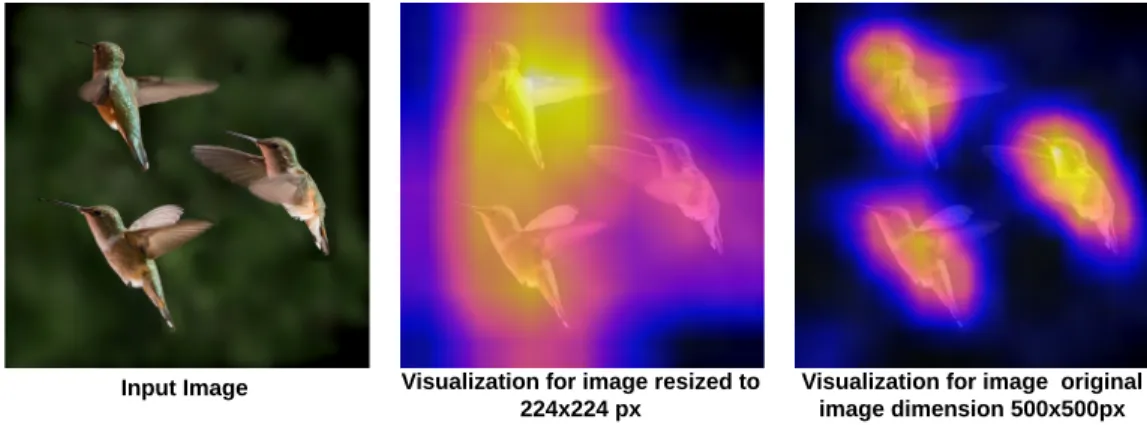
in [28]. However, that model uses multiple fully connected layers, requires using a sliding window method to process the image multiple times, and is trained with a multi-label training objective. In contrast, using fixed identity classifiers is fully convolutional and can handle input images of arbitrary size, and produces localization for all object categories in a single forward pass. This allows controlling the quality of the visualization simply by resizing the input during inference, as shown in Figure 5.4.
5.6
Attempts to improve the method
A few methods were explored to see if the results of the fixed identity classifier can be further improved.
Figure 5.2: Visualizations using fixed identity classifier with the ResNet-50 architecture fine-tuned on ImageNet-1K. Maximally activated classes are visualized for each object. Normalized scores and class labels are shown in the top-left corner of each visualization.
5.6.1 Orthogonal initialization and regularization
In this attempt, the network was either initialized using (semi-)orthogonal matrices (and broadcast into tensors in some cases), or applied soft orthogonality regularization or double soft orthogonality regularization as described in [2], using weight of 0.025. ResNet-18 is used as the base architecture, and the networks are trained on 100 category subset of ImageNet-1K. Results are given in Table 5.6. Unless otherwise mentioned, the parameters are initialized using uniform He initialization described in [8].
From the results, it is clear that neither orthogonal initialization or orthogonal regu-larization can further improve the performance of fixed identity classifiers.
Figure 5.3: Feature map visualizations for images contain multiple categories from ImageNet-1K.
5.6.2 Alternative pooling methods
Power-average pooling and soft attention pooling are also explored.
When using global power-average pooling in this setting, there is one parameterp, and the pooling is given as
g(f) = p
s X
f∈f
fp , (5.1)
where each element is power-averaged per channel. In the case ofp= 1, it is equivalent to sum pooling, which is proportional to average pooling; in the case ofp=∞it is equivalent to max pooling.
Input Image Visualization for image resized to 224x224 px
Visualization for image original image dimension 500x500px
Figure 5.4: CNN visualization for original image size (500px×500px) and resized (224px
×224px)
Table 5.6: Top-1 accuracy results of different orthogonal initialization and regularization configurations, using ResNet-18 as base on ImageNet-1K 100 category subset.
Orthogonal Initialization Orthogonal Regularization Top-1 Accuracy
None None 81.20%
Final Conv. Layer None 80.58%
All Conv. Layers None 77.44%
None Final Conv. Layer 80.24%
None All Conv. Layers 78.80%
Final Conv. Layer Final Conv. Layer 80.76%
In soft attention pooling, an additional module is created, it has two fully connected layers with tanh(·) as non-linear activation, and the number of hidden units is variable. It takes the flattened feature map as input, and the output goes through softmax(·) activation before being used weights for summing the feature maps.
Models based on the ResNet-18 architecture were trained for ImageNet-1K 100 cat-egory subset. Neither offers a significant boost to accuracy when using fixed identity
classifiers. For the sake of brevity, the detailed results are omitted. Furthermore, due to modifying the pooling operation, this makes free feature visualization unobtainable.
5.7
Summary
The fixed identity classifier was evaluated in multiple configurations, and compared against other fixed classifiers. In general, all fixed classifiers perform worse than a learned fully connected classifier. However, among the fixed classifiers, the fixed identity classifier performs best overall, while being the most simple method.
Discussions
This research is primarily driven by the work in fixed classifiers, which claims to be more efficient while maintaining performance [10]. In this research, fixed classifiers are put to the test, against learned classifiers, and also against the fixed identity classifier, which is equivalent to removing the fully connected classifier layer. This is an unorthodox approach, because traditionally CNN architectures have a feature extractor followed by a classifier. In the method proposed here, the classifier is removed, and classification scores are directly obtained from the last convolutional layer. Comparing to conventional networks, this is equivalent to removing the classifier; compared to fixed classifiers, this is equivalent to using an identity matrix as the fixed weights, which is a matrix that contains as little information as possible. This method can serve as a proxy to evaluate both learned fully connected classifiers, as well as fixed classifiers with specifically designed weights.
6.1
Benefits over other fixed classifiers
In all experiments that involve both fixed identity and fixed Hadamard classifiers con-ducted in this research, the fixed identity classifier outperforms the fixed Hadamard clas-sifier. This answers the question, whether fixed classifiers help the model learn anything. The results presented in this research show that specially designed weight matrices do not help the model learn to better classify. These designed fixed weights does force the feature extractor to produce features with specific characteristics, as presented in [29]. While also being capable of producing a classification score comparable to learned classifiers, it is actually worse than using a simple identity matrix.
While other Hadamard matrices exist (other than those constructed using the Sylvester’s method), Hoffer et al. does not use them in their source code. Also, they do not explain the rationale for why Hadamard matrices are beneficial, other than the fact that it does not require updating and is more efficient in terms of computation costs. Compute efficiency will be discussed later.
6.2
Parameter efficiency
On the large-scale ImageNet dataset and smaller CIFAR-100 dataset, along with two even smaller transfer learning datasets, the fixed identity classifier demonstrates it only suffers a relatively small sacrifice in accuracy, compared against learned classifiers, while saving a lot of parameters. Furthermore, on mobile architectures such as MobileNets and ShuffleNets that already reduce the total number of parameters required by a model, using a fixed identity classifier can reduce these memory requirements even further (e.g., 39% reduction for MobileNet v2 and 75% reduction for ShuffleNet V2, both on ImageNet) with only a
small degradation in performance, thus improving the parameter efficiency of models. There is a greater degradation of ImageNet-1K classification performance when using mobile architectures in conjunction with this method. In these scenarios, a significant amount of parameters are removed from the model, and in the case of ShuffleNet V2 x0.5, around 75% parameters are removed, leaving the model with only 0.3M parameters, compared to 1.3M parameters of the vanilla model. Results on ImageNet-100 showed that there is no performance degradation, which implies that the performance gap on ImageNet-1K is due to the model being too small to capture the statistics of the dataset. This suggests that while the final classifier layer uses a lot of parameters, it does not contribute much to the classification accuracy.
This means while fixed identity classifiers are not a drop-in replacement in some cases, the conventional approach of having a fully connected classifier is not very efficient in terms of the model size.
Furthermore, one could additionally make use of network pruning [1,7,11,20,21,24,36] to explicitly reduce parameters even further. Another option is to use network quantization to store parameters at a lower precision to save disk space and improve computational efficiency [5,14,15]. Also, it is possible to specifically promote sparsity in the final classifier using L1 regularization, using a learned final classifier.
While a lot of parameters can be saved in the final classifier, many models are very deep and wide, consisting of tens and even hundreds of millions of parameters. To these non-mobile models, the parameters in the fully connected final classifier can be negligible. It is debatable whether compressing the final FC layer is very useful in these scenarios. Despite this, as models get more complicated and are used for classification of datasets with an even larger number of categories, an alternative to a fully connected classifiers
Architecture Total First Conv. Final Classifier (FC) % FC ResNet-50 4.12G 118M 2.05M 0.05% ResNet-18 1.82G 118M 512K 0.03% MobileNet v2 320M 10.8M 1.28M 0.40% ShuffleNet V2 x0.5 43.6M 8.13M 1.02M 2.35% may be helpful.
6.3
Compute efficiency
One argument for using a fixed Hadamard classifier is that: 1) by not updating the weights during training 2) by using only +1 and -1 in the weights which simplifies calculation to use only inversions and summing , can significantly reduce computation costs. By using fixed identity classifiers proposed in this research, the cost for computation is even lower. However, by looking at a bigger picture, when taking into consideration the entire network, saving a single matrix-vector multiplication is negligible. Table 6.1 shows the compute requirements for different architectures in terms of floating-point operations.
As the numbers indicate, except for in ShuffleNet V2 x0.5, the final fully connected classifier layer uses more than 1% of the total compute, the FC layer uses a negligible amount of computation. And even in the case of ShuffleNet V2 x 0.5 which FC accounts for 75% of total parameters, the compute is only 2.35%.
Furthermore, while both Hadamard [10] and Binarized Neural Networks [5] argue for special hardware designs that can further improve efficiency, it is hard to imagine
a hardware that implements accelerated convolutions and general matrix multiplication (GEMM, level 3 BLAS) but does not have generalized matrix-vector multiplication (level 2 BLAS). Even if that is the case, it is not difficult to perform a single matrix-vector multiplication using the existing GEMM hardware.
6.4
Summary
While the fixed identity classifier yields comparable performance to a standard classifier when trained on ImageNet for all architectures tested, and completely outperforms other fixed classifiers in many ways, it still has a lot of limitations and pitfalls. It is incapable of handling more classes than the number of channels of output categories, which is the same for fixed Hadamard classifiers. It does reduce the computation requirements, but the effect is not very significant in the grand scheme of things in a deep CNN for image classification.
Despite the caveats of fixed identity classifiers, the results indicate that the final output layer does not need to be a learned fully connected layer. The final output layer in deep neural network architectures for image classification contains a lot of redundancy and can be greatly compressed for more efficiency. The results can be insightful for future efficient architecture design and/or efficient neural architecture search, enabling models to more easily scale to handle even larger datasets.
Conclusion
In this work, the performance and efficiency of various fixed classifier methods are eval-uated and compared against each other, and conventional learned classifiers. This work proposed the elimination of the fully connected classifier, and evaluated its performance on several modern CNN base architectures. By using global average pooling to compute classification predictions directly from the final convolutional layer, it is possible to achieve comparable performance to several CNNs that use a fully connected layer, while greatly reducing the total number of parameters required by the model, proving that specially de-signed fixed classifiers are not as effective as simply removing the final layer from networks, both in terms of parameter efficiency and classification accuracy. Research also showed that this approach is able to work on multiple datasets and neural network architectures. It is also demonstrated that using a fixed identity classifier is not only simpler, but also helpful in the visualization of the neural network features. It can generate visualizations similar to class activation maps, while requiring no additional post-processing.
This work also explored several methods that attempt to close the gap between this
fixed identity classifier method and learned fully connected classifiers. It was demonstrated that all these patchwork are of no avail.
Finally, this work demonstrated that the final classifier in general is not very efficient in terms of parameter size, and does not contribute very much to classification accu-racy. While it was discussed that neither of the alternative methods offers significant improvements in terms of computational efficiency, this work still suggests future neural architecture designs should use output layers more efficient than fully connected layers, in terms of parameter count.
Source Code (Selection)
A.1
Model Architectures
./models implementation/resnet cifar altskipconn.py
This implements more alternatives of the skip connection in the last block for ResNet-32.
1 import torch
2 import torch.nn as nn
3 import torch.nn.functional as F 4 import torch.nn.init as init 5 import random
6 from textwrap import dedent
7 import math
8 from models_implementation.clsf_utils import __fixed_eye, __no_bias, \
9 generate_hadamard, generate_orthoplex, generate_cube_ordered,
generate_cube_random ,→ 10 11 12 __all__ = [] 13 14 44
15 def _weights_init(m):
16 if isinstance(m, nn.Linear) or (isinstance(m, nn.Conv2d) and not
isinstance(m, FixedConv2d)):
,→
17 init.kaiming_normal_(m.weight) 18
19
20 class FixedConv2d(nn.Conv2d):
21 pass # just a hack to change signature 22
23
24 class LambdaLayer(nn.Module):
25 def __init__(self, lambd):
26 super(LambdaLayer, self).__init__() 27 self.lambd = lambd
28
29 def forward(self, x):
30 return self.lambd(x) 31
32
33 class BasicBlock(nn.Module): 34 expansion = 1
35
36 def __init__(self, in_planes, planes, stride=1, option='A'):
37 super(BasicBlock, self).__init__()
38 self.conv1 = nn.Conv2d(in_planes, planes, kernel_size=3,
stride=stride, padding=1, bias=False)
,→
39 self.bn1 = nn.BatchNorm2d(planes)
40 self.conv2 = nn.Conv2d(planes, planes, kernel_size=3, stride=1,
padding=1, bias=False)
,→
41 self.bn2 = nn.BatchNorm2d(planes) 42
43 self.shortcut = nn.Sequential()
44 if stride != 1 or in_planes != planes: 45 if option == 'A':
46 """
47 For CIFAR10 ResNet paper uses option A. 48 """
49 self.shortcut = LambdaLayer(lambda x: 50 F.pad(x[:, :, ::2, ::2], (0, 0, 0, 0, planes//4, planes//4), "constant", 0)) ,→ ,→ ,→ 51 elif option == 'B':
52 self.shortcut = nn.Sequential(
53 nn.Conv2d(in_planes, self.expansion * planes,
kernel_size=1, stride=stride, bias=False),
,→
54 nn.BatchNorm2d(self.expansion * planes)
55 )
56
57 def forward(self, x):
58 out = F.relu(self.bn1(self.conv1(x))) 59 out = self.bn2(self.conv2(out))
60 out += self.shortcut(x) 61 out = F.relu(out)
62 return out
63 64
65 class ClsfBlock(nn.Module): 66 expansion = 1
67
68 def __init__(self, in_planes, planes, stride=1, option='A',
num_classes=100):
,→
69 super(ClsfBlock, self).__init__()
70 self.conv1 = nn.Conv2d(in_planes, planes, kernel_size=3,
stride=stride, padding=1, bias=False)
,→
71 self.bn1 = nn.BatchNorm2d(planes)
72 self.conv2 = nn.Conv2d(planes, num_classes, kernel_size=3,
stride=1, padding=1, bias=False)
,→
73 self.bn2 = nn.BatchNorm2d(num_classes) 74 self.shortcut = nn.Sequential()
75 if stride != 1 or in_planes != num_classes: 76 if option == 'A':
77 """
79 """
80 pad_size = int((num_classes - in_planes)//2) 81 self.shortcut = LambdaLayer(lambda x:
82 F.pad(x, [0, 0, 0, 0, pad_size, pad_size], "constant", 0)) ,→ ,→ 83 elif option == 'B':
84 self.shortcut = nn.Sequential(
85 nn.Conv2d(in_planes, num_classes, kernel_size=1,
stride=stride, bias=False),
,→
86 nn.BatchNorm2d(num_classes)
87 )
88 elif option == 'C': # Hadamard and scaling
89 h = generate_hadamard(in_planes, num_classes) 90 h = h.view(num_classes, in_planes, 1, 1)
91 conv = FixedConv2d(in_planes, num_classes, kernel_size=1,
stride=stride, bias=False)
,→
92 conv.weight.data = h.float() 93 conv.weight.requires_grad_(False) 94
95 init_scale = 1. / math.sqrt(num_classes)
96 self.scale = nn.Parameter(torch.tensor(init_scale)) 97 self.shortcut = nn.Sequential(
98 conv,
99 LambdaLayer(lambda x: - self.scale * x), 100 nn.BatchNorm2d(num_classes)
101 )
102 elif option == 'D': # Fixed Orthoplex
103 w = torch.tensor(generate_orthoplex(in_planes,
num_classes))
,→
104 w = w.view(num_classes, in_planes, 1, 1)
105 conv = FixedConv2d(in_planes, num_classes, kernel_size=1,
stride=stride, bias=False)
,→
106 conv.weight.data = w.float() 107 conv.weight.requires_grad_(False) 108 self.shortcut = nn.Sequential(
110 nn.BatchNorm2d(num_classes)
111 )
112 elif option == 'E': # shuffled fixed Orthoplex, using all
channels at least once (64x +1 then 36x -1) ,→
113 w = torch.zeros(num_classes, in_planes) 114 for row in range(num_classes):
115 col = row % in_planes
116 w[row, col] = 1 if row < in_planes else -1 117 w = w .view(num_classes, in_planes, 1, 1)
118 conv = FixedConv2d(in_planes, num_classes, kernel_size=1,
stride=stride, bias=False)
,→
119 conv.weight.data = w.float() 120 conv.weight.requires_grad_(False) 121 self.shortcut = nn.Sequential(
122 conv,
123 nn.BatchNorm2d(num_classes)
124 )
125 elif option == 'F': # d-cube ordered 126 w = generate_cube_ordered(64, 100)
127 w = w.view(num_classes, in_planes, 1, 1)
128 conv = FixedConv2d(in_planes, num_classes, kernel_size=1,
stride=stride, bias=False)
,→
129 conv.weight.data = w.float() 130 conv.weight.requires_grad_(False) 131 self.shortcut = nn.Sequential(
132 conv,
133 nn.BatchNorm2d(num_classes)
134 )
135 elif option == 'G': # d-cube random 136 w = generate_cube_random(64, 100)
137 w = w.view(num_classes, in_planes, 1, 1)
138 conv = FixedConv2d(in_planes, num_classes, kernel_size=1,
stride=stride, bias=False)
,→
139 conv.weight.data = w.float() 140 conv.weight.requires_grad_(False) 141 self.shortcut = nn.Sequential(
143 nn.BatchNorm2d(num_classes)
144 )
145 elif option == 'H': # d-cube some better ordering that I can
think of ,→
146 raise NotImplementedError # don't know how to do it yet
147 else:
148 raise NotImplementedError 149
150 def forward(self, x):
151 out = F.relu(self.bn1(self.conv1(x))) 152 out = self.bn2(self.conv2(out))
153 out += self.shortcut(x)
154 return out
155 156
157 class ResNet_alt(nn.Module):
158 def __init__(self, block, num_blocks, num_classes=100, option='A'):
159 super(ResNet_alt, self).__init__() 160 self.clsf_expansion_option = option 161 self.in_planes = 16
162 self.conv1 = nn.Conv2d(3, 16, kernel_size=3, stride=1, padding=1,
bias=False)
,→
163 self.bn1 = nn.BatchNorm2d(16)
164 self.layer1 = self._make_layer(block, 16, num_blocks[0],
stride=1)
,→
165 self.layer2 = self._make_layer(block, 32, num_blocks[1],
stride=2)
,→
166 self.layer3 = self._make_layer(block, 64, num_blocks[2],
stride=2, num_classes=num_classes)
,→
167 self.fc = nn.Linear(100, num_classes) 168 self.apply(_weights_init)
169
170 def _make_layer(self, block, planes, num_blocks, stride,
num_classes=None):
,→
171 strides = [stride] + [1]*(num_blocks-1) 172 layers = []
174 if (num_classes is not None) and (idx == len(strides) - 1): 175 layers.append(ClsfBlock(self.in_planes, planes, stride,
self.clsf_expansion_option, num_classes))
,→
176 else:
177 layers.append(block(self.in_planes, planes, stride)) 178 self.in_planes = planes * block.expansion
179
180 return nn.Sequential(*layers) 181
182 def forward(self, x):
183 out = F.relu(self.bn1(self.conv1(x))) 184 out = self.layer1(out)
185 out = self.layer2(out) 186 out = self.layer3(out)
187 out = F.avg_pool2d(out, out.size()[3]) 188 out = out.view(out.size(0), -1)
189 out = self.fc(out)
190 return out
191 192
193 for option in ['a', 'b', 'c', 'd', 'e', 'f', 'g']: 194 code = f"""\
195 def rn32_cf100_ex{option}():
196 model = ResNet_alt(BasicBlock, [5, 5, 5],
option='{option.upper()}') ,→
197 return model
198
199 def rn32_cf100_ex{option}_fixed_eye(): 200 model = rn32_cf100_ex{option}()
201 model = __fixed_eye(model)
202 return model
203
204 def rn32_cf100_ex{option}_no_bias(): 205 model = rn32_cf100_ex{option}()
206 model = __no_bias(model)
207 return model
209 def rn32_cf100_ex{option}_fixed_eye_no_bias(): 210 model = rn32_cf100_ex{option}()
211 model = __no_bias(model)
212 model = __fixed_eye(model)
213 return model
214 """
215 exec(dedent(code))
216 __all__ += [f'rn32_cf100_ex{option}',
f'rn32_cf100_ex{option}_fixed_eye',
,→
217 f'rn32_cf100_ex{option}_no_bias',
f'rn32_cf100_ex{option}_fixed_eye_no_bias']