An evaluation of the consistency of extremes in gridded precipitation data sets

Recent Work

Title

An evaluation of the consistency of extremes in gridded precipitation data sets

Permalink

Authors

Publication Date

DOI

https://doi.org/10.1007/s00382-018-4537-0

An evaluation of the consistency of extremes in gridded precipitation

data sets

Ben Timmermans1  _{· Michael Wehner}1 _{· Daniel Cooley}1 _{· Travis O’Brien}1 _{· Harinarayan Krishnan}1

Received: 2 March 2018 / Accepted: 13 November 2018 © Regents of the University of California 2019

Abstract

Noting a strong imperative to understand precipitation extremes, and that considerable uncertainty affects observational data sets, this paper compares the representation of extremes in a number of widely used daily gridded products, derived from rain gauge data, satellite retrieval and reanalysis for the conterminous United States. Analysis is based upon the concept of “tail dependence” arising in multivariate extreme value theory, and we infer the level of temporal dependence in the joint tail of the precipitation probability distribution for pairwise comparisons of products. In this way, we consider the range of products more like an ensemble and examine the relationships between members, and do not attempt to define, or compare products to, some ground truth. Linear correlation between products is also computed. Considerable discrepancy between groups of products, both annually and seasonally, is linked to source data and complex terrain. In particular, products based on rain gauge data showed remarkable similarity, but differed considerably, showing almost total loss of extremal dependence during DJF in mountainous regions, when compared with satellite products. Additionally, simulated re-forecasts revealed reason-able temporal agreement with large scale generated extremes. The diversity and extent of discrepancies identified across all products raises important questions about their use, and we urge caution, particularly for products derived from satellite data.

Keywords Precipitation · Extremes · Gridded products · Extreme value theory · Tail dependence · Comparison

1 Introduction

There is huge research interest in observational records of precipitation that spans environmental and hydrological modeling, climate change and resource and risk management (Groisman et al. 1999; Krishnamurthy and Shukla 2000; Alexander et al. 2006; Schar et al. 2016). Understanding variation in precipitation—particularly the extremes—is critical for resource and emergency management, especially in the face of droughts and floods in a changing climate. The quality of the observational record is therefore also critical.

Obtaining a complete spatio-temporal record of precipita-tion is, however, not straightforward. Typically, networks of

ground-based instruments providing in-situ measurements have the longest observational records although since the 1980s these have been augmented by a range of satellite based radar platforms. Ground based radar is also a valuable measuring system for some applications. Further details of various observational approaches are described, for example, by Michaelides et al. (2009) and Tapiador et al. (2012). No single measurement approach yet provides a reliable and complete spatio-temporal record, which in part motivates the need for quality controlled compiled data sets. The two broad categories of measurement system used for large scale observations, rain gauge networks and satellite based radar, each suffers from its own set of limitations. Rain gauges can provide an accurate and continuous record at a single loca-tion, although they may be affected by a variety of errors, including undercatch (Groisman and Legates 1994; Chvila et al. 2005; Kochendorfer et al. 2017). They may also suf-fer from variance in management quality (Viney and Bates

2004) and discontinuity due to changes in equipment or location (Leeper et al. 2015). Rain gauges tend to be fairly abundant in developed countries (Menne et al. 2012; Yatagai et al. 2012) but nonetheless the biggest, and most obvious Electronic supplementary material The online version of this

article (https ://doi.org/10.1007/s0038 2-018-4537-0) contains supplementary material, which is available to authorized users.

* Ben Timmermans

[email protected]

1 _{Lawrence Berkeley National Laboratory, 1 Cyclotron Road,}

problem is the lack of spatial coverage. This can be exac-erbated by the inaccessibility of remote or hostile terrain. Much of the western US, for example, is characterized by complex topography. The observational data must therefore be interpolated in some way (Thornton et al. 1997; Xie et al.

2007; Hofstra et al. 2008; Zolina et al. 2014), often involving spatial methods related to kriging (Cressie 1993). Interpo-lated values at unobserved locations are therefore subject to uncertainty from measurement error and the interpola-tion method, both of which can be a strong funcinterpola-tion of oro-graphic variability and regional atmospheric characteristics (Roe 2005; Lundquist et al. 2010; Boers et al. 2016). Over more recent decades satellite-born radar has been able to provide spatially and temporally continuous observations across the globe (Maggioni et al. 2016). Continuous cover-age is desirable, but difficulties are introduced because pre-cipitation is not measured directly but inferred from micro-wave and infrared radar measurements, thus adding another layer of data processing that is subject to uncertainty and error (Iguchi et al. 2009; Tapiador et al. 2012). Nonetheless, these measurements are valuable where ground based obser-vations are sparse, and they have received much attention in the research community (Behrangi et al. 2011; Jiang et al.

2012; Xue et al. 2013; Blacutt et al. 2015; Miao et al. 2015; Conti et al. 2014; Ma et al. 2016).

In order to make data access more practical, and also to incorporate post-processing of the raw observations, a large number of geographically gridded precipitation products (referred to hereafter as “products”) have been developed. Global products may cover only the land surface (Adler et al.

2003; Fick and Hijmans 2017; Schneider et al. 2017) but depend on satellite retrieval for complete coverage (Joyce et al. 2004; Huffman et al. 2007; Ashouri et al. 2015; Xie et al. 2017). Regional products are typically more diverse (and numerous) (Chen et al. 2008; Xie et al. 2007; Thornton et al. 1997; Livneh et al. 2013; Haylock et al. 2008; Auer et al. 2007; Herrera et al. 2016; Rauthe et al. 2013; Yatagai et al. 2012; Greene et al. 2008), and may incorporate some combination of direct measurement and radar. Applications of these products are extensive and diverse including direct studies of the data (Lambert et al. 2004), numerical model validation (Gervais et al. 2014a) and model input (Xue et al.

2013; Dalhaus and Finger 2016). Clearly gridded products are a key element in the evaluation of climate models that generate output on similar grids (Wehner 2013; Chen et al.

2013b; Sunyer et al. 2013; Kotlarski et al. 2014; Mehran et al. 2014; Gervais et al. 2014a). This alleviates the need to process gridded model output into a point format for comparison with a gauge network, although a transforma-tion from point-to-grid, or vice-versa is required, and simi-lar uncertainties are introduced in either case. In addition to observational products, reanalysis data, generated via the assimilation of observations into numerical weather

forecasts, provide another source of precipitation data for comparison (Mesinger et al. 2006; Rienecker et al. 2011; Dee et al. 2011).

While all of these products are valuable to the research community, their use motivates some important questions. Firstly, is uncertainty information available, and is it robust? Secondly, given the importance of precipitation extremes, how well are the extremes represented? This paper primarily focusses on addressing the second question by intercom-paring a range of products. However, before describing our approach we briefly discuss the more general issue of uncertainty.

Stronger focus on uncertainty is a growing trend in grid-ded product development (Woldemeskel et al. 2013; Zolina et al. 2014; Isotta et al. 2014; Daly et al. 2017). Some, par-ticularly more recent products including GPCP (Adler et al.

2003), the ensemble product of Newman et al. (2015) and Daymet (Thornton et al. 2016), explicitly make available uncertainty information. However, many do not do so (CPC, Livneh, PRISM, NARR), and even where such information is available its use is not always straightforward. Newman et al. (2015), for example, provide 100 ensemble members, each 16 GB in size, making its use far from convenient. For satellite products, rigorous uncertainty estimates are more difficult to obtain, being a function of many sources including data and processing algorithms that are subject to regular recalibration (Ashouri et al. 2015). The diversity of products available, their respective approaches to uncer-tainty estimation (if any) and the absence of a comprehen-sive analysis, leaves product selection a considerable chal-lenge. Nonetheless, more limited case-by-case studies often intercompare one or more products, usually on a regional basis (McAfee et al. 2014; Salio et al. 2015). A few studies have attempted to address this issue more comprehensively (Behnke et al. 2016; Henn et al. 2017). In particular, Henn et al. (2017) examine six publicly available gridded prod-ucts by evaluating measures including the mean and rela-tive difference in annual total precipitation. Geographically, they focus on complex elevated terrain, where in general products are known to show discrepancy, and they reveal a range of systematic differences between products in all evaluation metrics. A limited comparison with independent observations (stream flow data) also suggests that uncer-tainty derived from all products may be an underestimate and like other studies, they caution users to be critical when selecting a product for use. The apparent lack of a clearly identifiable ground truth product raises questions about how to proceed with performance evaluation and product intercomparison. An ensemble approach would seem natu-ral, analogous to studies of numerical simulations (Gleckler et al. 2008; Sanderson et al. 2017), where member products can be treated equally or weighted according to prior infor-mation, perhaps based upon some measure of performance.

Similar approaches have been applied in the creation of observational data sets (Beck et al. 2017) and evaluations of methodologies for describing precipitation over specific regions (Pena-Arancibia et al. 2013). However, our objective is not to investigate in detail the sources of uncertainty in individual products or identify the most accurate product on this basis. In some sense, available products in totality may be considered the “ground truth” and as such, in this paper we propose to examine relationships between them. With this in mind, we return to the question of the representation of extremes.

Extremes of precipitation have been studied in numerous cases (Groisman et al. 1999; Alexander et al. 2006; King et al. 2013; Miao et al. 2015; Gervais et al. 2014b; Con-tractor et al. 2015; Behnke et al. 2016), most often where a gridded product is compared to some “truth”—usually direct measurements from high quality rain gauge data. The defini-tion of extreme can include measures defined directly from an empirical probability distribution, such as quantiles, and more practical metrics such as number of consecutive wet days. The extremal measure is also a function of the duration of the available data which must be considered. While some rain gauge data exceeds 100 years, often data sets are around 20–30 years in duration, limited by satellite records or drawn from managed observational networks that have been imple-mented more recently. In practice, the definition of extreme can vary considerably. Zhang et al. (2011) discuss indices for extreme precipitation at length, in the context of examining long term trends in extremes and the attribution of extremes to anthropogenic influence. While cautioning the use of grid-ded products for the study of extremes, they also discuss the problem of converting point observation data to grid cells (typically for comparison with numerical simulation output). This issue is also investigated by Gervais et al. (2014b) who explicitly quantify errors in extreme precipitation introduced by gridding methodology as a function of target resolution and station density. Choice of methodology is reported to contribute up to a 30% difference. They emphasise the importance of station density and in particular how this is a function of geographic location where terrain and physical processes are variable. Like Zhang et al. (2011) they also discuss the important issue of the relationship between point observation and an areal average—analysis must be applied consistently in order to correctly conserve quantities. Other studies examine the use of gridded products to investigate both mean and extremes (Behnke et al. 2016; Contractor et al. 2015; King et al. 2013). King et al. (2013) in particular investigate the efficacy of using a high resolution gridded product to analyse trends in extreme rainfall and conclude that while viable, caution must be adopted. They recommend that products be tested in order to identify areas of weakness, such as low station density, where interpolation methods tend to perform poorly.

As discussed earlier, in contrast to these other studies, in this paper we examine the representation of precipitation extremes in gridded products without attempting to define a ground truth. We intercompare a range of widely used products for the CONUS in a pairwise approach using meth-ods from bivariate extreme value theory. More specifically, between pairs of products we infer empirically the level of asymptotic dependence—dependence in the extremes. Our analysis is related to that used in weather forecast scoring and verification (Stephenson et al. 2008). The approach examines relationships between products consistently, revealing key similarities and differences which can guide further exploration and analysis. A wide ranging intercom-parison of this type thus reveals information that is less clear when analysis is limited to a small number of products or focusses closely on the details of a single methodology. In addition to the observational products, we also include in the analysis a simulated re-forecast data set that provides useful insight into modeling issues. As far as we are aware this is the first study to make use of extreme value theory in this way with respect to observational data sets.

The structure of this paper is as follows. In Sect. 2, we describe the gridded products used in the analysis. Section 3

describes our methodology including relevant aspects of extreme value theory. Our results are presented in Sect. 4

with following discussion in Sect. 5, and conclusions in Sect. 6.

2 Datasets

Our study area is the CONUS for which there are numer-ous gridded products available. All products used provide daily precipitation totals at native spatial resolutions rang-ing from approximately 1–25 km. The ten products and one simulation data set examined in this paper are listed in Table 1. For the analysis, products were (re-)gridded to the native grid for the (Climate Prediction Center) CPC data set, which is rectilinear at 1∕4◦_×1∕4◦ . A bilinear

interpo-lation method was applied to those products provided on a rectilinear grid (Maurer, Livneh, ERA, ILIAD), otherwise the area-conservative method of the Earth System Mod-eling Framework (Hill et al. 2004) was employed. TRMM, CMPORPH, PERSIANN and CPC all use coincident grids by default. We conducted a pairwise analysis that required time series of equal length, therefore the length of each paired data set was constrained by the mutually latest start and earliest end dates. This is not problematic for our extre-mal analysis methodology because it is not dependent on time series length, but shorter series, and hence fewer data, result in greater uncertainty (see Sect. 3.1 for more details). It is beyond the scope of this work to go into the details of the gridding methodology for each product, which are

numerous; however, we briefly summarize. The CPC uni-fied gauge-based analysis of daily precipitation over CONUS is based upon an optimal interpolation approach following (Gandin and Hardin 1965). The Maurer and Livneh data sets, the latter being a revised and lengthened version of the former, employ a variant of an inverse distance and direc-tional weighting scheme (Shepard 1968). The resulting grids for both of these approaches are calibrated against PRISM monthly climatological values. The PRISM (Precipitation-Elevation Regressions on Independent Slopes Model) prod-uct itself is generated from the PRISM algorithm that, in common with CPC, uses a linear regression approach com-bining gauge data by weighting based upon factors such as location, elevation, coastal proximity, topographic facet orientation and others. Daymet uses a different approach based upon spatial convolution, described by Thornton et al. (1997). Source data for the gauge-based products is varied but there is considerable overlap. Both the CPC and Livneh products incorporate daily totals from the National Oceanic and Atmospheric Administration (NOAA) coopera-tive observer stations. The Global Historical Climatology Network-Daily (GHCN-D) dataset (Menne et al. 2012), or subsets thereof (subject to quality control, for example), are often used. It would be reasonable to expect that these prod-ucts are highly correlated noting the often common input data and similar interpolation schemes.

Satellite based products also vary considerably in terms of their source data and processing algorithms. They have gone through many revisions, which incorporate data from different instruments and satellites. See e.g. Maggioni et al. (2016), Huffman et al. (2007), Joyce et al. (2004), Chen et al. (2013a) and Xie et al. (2017). PERSIANN is somewhat unique here in that it combines both rain gauge and satel-lite data. Reanalysis data, derived principally from simu-lated weather forecasts, may incorporate both rain gauge

and satellite precipitation, along with a range of other cli-matic variables, through a data assimilation scheme. With relevance to this study, the NARR (Mesinger et al. 2006) assimilates principally CPC (rain gauge) precipitation data over land, and satellite-derived data over coastal and oceanic regions, whereas the ERA global product (Dee et al. 2011) assimilates only from satellites. In particular they discuss difficulties, such as excessive tropical rainfall, when deriving precipitation rates from satellite observed infrared radiances, covered also by Uppala et al. (2005).

The InitiaLIzed-ensemble, Analyze, and Develop (ILIAD) framework (O’Brien et al. 2016) was used to gen-erate a five year time series of re-forecasts in order to com-pare observed and simulated weather events across multiple resolutions. It employs the Community Earth System Model (CESM), initialized by the US National Center for Environ-mental Protection (NCEP) reanalysis data set. Since each day is initialised from reanalysis, the simulated state of the atmosphere is constrained to remain close to the observed state. The output data set used here comprises a 5 year time series of the 4th-day forecast. Note that 5 years is substan-tially shorter in duration than the other data sets considered in this study, which gives rise to a higher variance in the sta-tistical estimates that we generate (see Sect. 3). The detailed analysis of simulation output is not within the scope of this study but the inclusion of a simulated data set provides a useful comparison.

3 Methodology

Our investigation examines variability in the correspondence of extreme precipitation events by analysing pairs of grid-ded data products. Comparison of data sets often involves summary measures such as correlation. While correlation is Table 1 Gridded precipitation

products and data sets assessed over the CONUS

Letters of the fourth column designate (G)auge data, (S)atellite data, (C)ombined sources (e.g. both gauge and satellite), (R)eanalysis and (M)odel output

Product name (reference) Original resolution First-last (total) years Data type CPC (http://www.esrl.noaa.gov/psd/data/gridd

ed/data.unifi ed.daily .conus .html)

1_∕4◦ 1950–2017 (68) G

Maurer (Maurer et al. 2002) 1_∕8◦ 1950–1999 (50) G

Livneh (Livneh et al. 2013) 1∕16◦ 1950–2011 (62) G

PRISM (Daly et al. 2008) 4 km ( ∼1_∕25◦₎ 1981–2017 (37) G

Daymet (http://dayme t.ornl.gov/overv iew.html) 1 km ( ∼1_∕100◦₎ 1980–2017 (38) G

TRMM V7 (Huffman et al. 2007) 1_∕4◦ 1998–2017 (20) S

CMORPH 1.0 (Xie et al. 2007) 1∕4◦ 1998–2017 (20) S

PERSIANN-CDR (Ashouri et al. 2015) 1_∕4◦ 1983–2017 (35) C

NARR (Mesinger et al. 2006) 1_∕4◦ 1979–2015 (37) R

ERA-Interim (Dee et al. 2011) 1∕4◦ 1979–2015 (37) R

influenced by the extremes, it is a summary of the whole of the data and is of much less use in making statements about the extremes in particular. Our approach employs methods derived from extreme value theory that share a connection with weather forecast verification, where two data sets— the prediction and observation—are compared statistically (discussed further at the end of this section and in Sect. 5). In contrast to that example we focus on comparing pairs of data sets where both are representations of reality. We do not therefore define a “ground truth” against which comparisons can be made nor do we attempt to determine the quality or accuracy of any individual data set in an absolute sense. However, our approach focusses on the extremes, and by considering each data set as an ensemble member we build a picture of the structure of the representation of extremes within the ensemble.

In the remainder of the section we provide a summary of the statistical methods employed.

3.1 Extreme value theory

Extreme value theory provides a framework for studying the upper (or lower) tail of a probability distribution. There is an extensive literature covering this topic and the reader is directed to Coles (2001), Weller et al. (2012) and references therein for in-depth discussion. Davison and Huser (2015) provide an up-to-date review of the use of extreme value theory in current research topics.

In weather and climate research it is common to see anal-ysis of the lower order moments of a population distribution but perhaps less so of the tails of the distribution. We there-fore start by emphasising the important distinction between the two regimes. Gaussian distributed data exhibit exponen-tially decaying tails and so the probability of samples from such a population lying much beyond three standard devia-tions becomes vanishingly small. However, many physical variables, such as precipitation or the height of ocean waves exhibit probability distributions with tails that decay more slowly. Observations lying many standard deviations from the mean may occur with appreciable probability. Given a population characterized by a heavy-tailed distribution, the observation of a new extreme event could have a substantial influence on estimates of further extremes. Accurate estima-tion of the behavior of the tail is crucial to, for example, esti-mates of return times for high magnitude weather extremes upon which the safe design of infrastructure relies. Extreme value theory therefore provides us a statistical framework in which we can study extremes.

Univariate extreme value theory is often employed to investigate the properties of climate extremes (Weh-ner 2013; Timmermans et al. 2017). Typically a param-eterized extreme value probability distribution is fitted to the extremes of the data set using a block-maxima or

peaks-over-a-high-threshold method (Coles 2001; Davi-son and Smith 1990). The fitted model can then be used for statistical inference about extremal properties, such as long return times. However, this paper presents a dif-ferent kind of application by making use of methods from bivariate extreme value theory. The approach is similar in concept to an analysis of the correlation between two data sets. For the extremes of data however, correlation is inap-propriate because it considers the totality of the data. In fact, a particularly important topic in multivariate extreme value theory is how to model the possible range of classes of extremal dependence. More specifically, two general cases exist: asymptotic dependence and asymptotic independence. In practice, the two cases can be difficult to distinguish for-mally but it is important to understand the difference and the implication of each regime. For correlated variables, if one underestimates the correlation, the joint probability of two events will be underestimated. In the same way, a mischaracterization of extremal dependence can lead to an underestimate of the joint probability of extremes. To use a practical example, if one were designing coastal defenses, knowledge of the joint probability of high waves and heavy rainfall—both related to flooding—would be critical. Robust inference for the asymptotic behavior between wave height and rainfall would therefore be required. We refer the reader to Coles (2001) (chapter 8), Ledford and Tawn (1996) and Wadsworth et al. (2017), for further details about bivariate extreme value theory beyond what we cover below. Suppose (X, Y) is a pair of random variables whose joint tail behavior we wish to characterize. Because X and Y can have different behavior and more specifically can become extreme at very different values, it is typical to account for marginal behav-ior before characterizing extremal dependence. This is not too different from correlation which accounts for marginal behavior by accounting for the variance of each variable. Let F_X(x) =P(X≤x) be the cumulative distribution function

(cdf) of X and similarly for Y. It is well known that apply-ing the cdf to the random variable results in a Uniform[0,1] random variable; that is P(F_X(X)≤q) =q for 0≤q≤1 . A

parameter that describes extremal dependence is,

which has the straightforward interpretation of the prob-ability that X is at its most extreme levels given that Y is at its most extreme levels. 𝜒 is a measure of the strength of

dependence in the asymptotic dependent setting, and asymp-totic independence corresponds to 𝜒=0 . If X and Y are

independent then they are also asymptotically independent. However the converse is not true; if (X, Y) are Gaussian with correlation 𝜌 <1 , they are asymptotically independent.

(1)

𝜒=lim

q→1P(FX(X)>q∣FY(Y)>q) =limq→1

P(FX(X)>q,FY(Y)>q) P(FY(Y)>q)

Since 𝜒 is defined as a limit, it is challenging to

esti-mate. One wants to limit one’s attention to only the very largest observations of each variable, and at the same time one needs to have an adequate number of observa-tions to perform estimation. Standard practice is to define

̂

𝜒(q) =P̂(F_X(X)>q∣F_Y(Y)>q) where P̂ denotes an

esti-mated probability, and obtain estimates of 𝜒(q)̂ for

increas-ing values of q approaching 1. We estimate 𝜒̂(q) using the chiplot function in R’s evd library, which uses an esti-mator provided by Coles et al. (1999). This estimator uses a copula approach which takes advantage of symmetry arising from the fact that the denominator in the right-most expres-sion in (1) can be replaced by P(FX(X)>q).

We now demonstrate the use of 𝜒 when examining

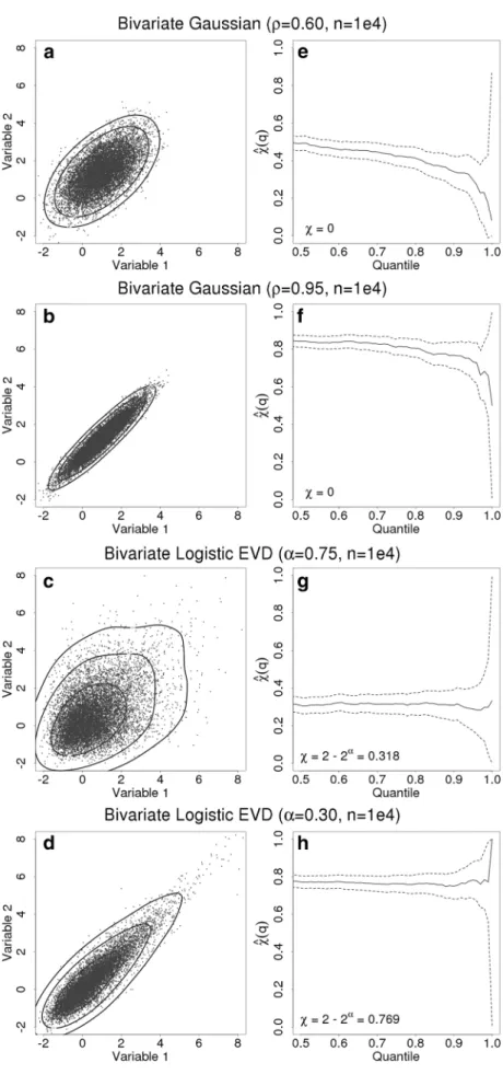
extre-mal dependence in some synthetic bivariate data sampled from two different families of distributions. We illustrate asymptotic independence by analyzing bivariate Gaussian random variables. To illustrate asymptotic dependence, we simulate data from a bivariate logistic distribution (see Coles

2001) which has a distribution function given by,

For this distribution, the true (that is the limit as q→0 )

value of 𝜒=2−2𝛼 . Samples of size _n=1e4 are shown in

Fig. 1a–d and their corresponding “ 𝜒-plots” in Fig. 1e–h.

Empirical density contours, derived from kernel density estimation, have been added for purposes of comparison. Firstly, samples are drawn from two bivariate Gaussian dis-tributions defined such that correlation 𝜌=0.60, 0.95 , shown

in Fig. 1a, b respectively. In both cases we draw attention to the lack of points in the upper right quadrant of the figures, much greater than the mean, consistent with the exponential decay of probability density. This is also clear from the lack of samples anywhere far from the joint 0.99 quantile line. Even in cases of strong correlation, asymptotic independ-ence implies that the dependindepend-ence between jointly Gaussian random variables weakens (in the sense of 𝜒 ) as one looks

further and further into the tail. This reinforces the need to consider extremes in a rather different way to the lower order moments. Samples from the logistic bivariate extreme value distribution (2) for 𝛼=0.3, 0.75 are shown in Fig. 1c, d. In

contrast to the Gaussian cases we now see sampled points lying in the upper right quadrant far beyond the joint 0.99 quantile contour, indicative of a heavy joint tail. The differ-ence in strength of dependdiffer-ence is clear from the more tightly constrained tail in Fig. 1d.

Figure 1e–h show 𝜒̂(q) plotted against quantile, q, which

provides a means of quantifying the strength of depend-ence, under the assumption of asymptotic dependence. If

̂

𝜒(q) tends to zero in the limit of the data then we can assume 𝜒 =0 and that the data are asymptotically independent. Note

that the expression for the confidence intervals, which is (2)

P(X≤x,Y ≤y) =exp[−(x−1∕𝛼+y−1∕𝛼)𝛼_{], x>0, y>0.}

proportional to 𝜒 and the square root of the sample size, is

derived using the delta method (see Coles et al. 1999). On inspection, a degree of interpretation is required, particularly noting that the 95% confidence limits (dashed lines) grow as the data becomes sparse towards the limit. The sample size n=1e4 is approximately equivalent to 30 years of daily

observations. In Fig. 1e, f we might have reason to suspect asymptotic independence, since the trend appears to have a negative gradient although even for highly correlated Gauss-ian data, the confidence limits bound a constant trend in 𝜒

even into the high quantiles. Figure 1g, h suggest a more stable trend. For comparison, samples of size n=3e3 ( ∼

9 years) and n=1e5 ( ∼ 275 years) for both Gaussian and

bivariate logistic distributions are shown in Figure S1 (in the supplementary information). In cases where only 10 years of observations are available (with fewer, in the ILIAD data set, having been used in this study), the large estimation uncer-tainty should dictate caution. The challenge of determining asymptotic dependence or independence is an active area of statistical research and lies beyond the scope of this paper. For purposes here, it is important to have an understanding of these two regimes and, most importantly, to know that familiar measures of dependence have no value in describing extremal dependence.

To motivate studying extremal dependence we ear-lier spoke of the need to estimate the probability of joint exceedances, such as with our coastal defense example. In this work, we will use 𝜒 for an entirely different and

novel purpose: to compare extremes between observational data sets. It stands to reason that two observational data sets should exhibit asymptotic dependence since both are based on observations of the same weather, and therefore should exhibit extreme behavior at the same time. While 𝜒

has not previously been used to compare extremes between observational data sets, examples of similar studies of tail dependence have been presented in the literature. Weller et al. (2012) used 𝜒 to compare observations to model

out-put, and Stephenson et al. (2008) used a related measure for weather forecast verification. Kuhn et al. (2007) also evalu-ated tail dependence in an investigation of spatial precipita-tion extremes in South America.

3.2 Approach

Having described measures for the assessment of observa-tional data extremes we now address their application to precipitation products. Our objective is to infer extremal dependence between pairs of data sets. Gridded products generally provide complete spatial and temporal coverage within their designated domain (occasionally exceptions to this occur—we found a corrupt day of data in 1952 in CPC, and a few data gaps largely outside the CONUS in all satellite products). Thus, when undertaking a pairwise

Fig. 1 Samples drawn from parameterized bivariate distri-butions (a–d) and correspond-ing computation of 𝜒̂(q) with

analysis, each spatial grid cell provides a bivariate distri-bution from which we can infer extremal dependence using the methods described in Sect. 3.1. Since 𝜒(̂ q) is exhibits

high variability for q near 1, and to reduce the 𝜒̂(q) plot

to a single number for comparison between products, we compute 𝜒̂(q) , averaged over an interval at a high quantile.

Specifically,

Equation (3) therefore captures correspondence in the high quantiles but attempts to minimize the effect of uncertainty as data becomes sparse.

We apply (3) to the complete continuous bivariate time series formed by each pair of products, where the length of the time series is dictated by the coincidence of mutual start and end dates. As such, some data is discarded in all analyses since no pair of products coincide for their entire record. The longest period of coincidence is between CPC and Livneh (62 years) with the shortest being comparisons with Iliad (5 years). We have also considered seasonality based on winter (DJF) and summer (JJA) months. In these cases 𝜒̂∗ is computed only for the continuous time series

of those months during each year. Given all products aim to capture the historical record, we anticipate good agree-ment between the products and that asymptotic depend-ence will be strong.

We emphasize here a few important aspects of our analysis. Only temporal dependence is evaluated, and we treat geographic location marginally (i.e. treating grid cells independently). Furthermore, use of (3) does not account for differences in (temporal) marginal behav-ior, obviated by the use of a copula based estimator that involves transformation of the (two) input precipitation data sets to uniform marginal distributions. We can thus say nothing about the differences in shape of the marginal distributions, or their tails, between products, such as the absolute magnitude of the extremes, however, many stud-ies typically undertake such analysis, and our approach is complimentary in that sense.

Another relevant issue is that of possible non-station-arity in one or both time series. In studies of precipitation climatology, non-stationarity of the climate system, such as that induced by human influence, is typically of interest and trends in both mean and extremes with regional vari-ation have been identified for the CONUS (Kunkel et al.

2013; Easterling et al. 2017). If extremal dependence is a function of such trends, then extremal analysis could be affected, in particular because some comparisons are con-ducted over different time periods due to the availability of data. However, a temporal trend due to climate change should not affect 𝜒 as it measures whether extremes occur

(3) ̂ 𝜒∗ ∶= ∑ 0.90<q≤0.95 ̂ 𝜒(q),

concurrently, which can be separated from marginal behavior. Furthermore, climate change induced trends over the observation periods we have available are small. We explore these issues further, in Sect. 4.4 and in the supplementary information (Text S1 and Figures S4, S5).

3.3 Computational aspects

𝜒 is very cheap to compute for a bivariate daily time series

over many decades, using the evd for R (https ://cran.r-proje ct.org/web/packa ges/evd), for example. However, when working with gridded data sets in high dimension this becomes fairly expensive. We employed a high performance computing platform running R in parallel using pbdR (Ost-rouchov et al. 2012) to perform the analysis. Each analysis took between approximately one and two hours on 32 pro-cessing cores.

4 Results

4.1 Temporal considerations

We begin by highlighting how inconsistent handling of observation timing can introduce artifacts and errors into gridded data sets. We found that comparisons between the Maurer, Livneh and CPC data sets (those derived explicitly from rain gauges) revealed temporal inconsistencies on the daily time scale. In particular, when comparing Maurer and CPC, it is easily seen that a lag has been introduced. Figure 2

shows scatter plots for two different locations: California (lon. − 121.2, lat. 39.8); Kansas (lon. − 99.3, lat. 37.2). Figure 2a shows strong correlation throughout the range of the data for California (this trend is fairly consistent for the west coast). However, Fig. 2b shows very poor correlation in Kansas. In fact, the structure of the data is indicative of a data set plotted against a lag of itself. We can recover much higher correlation by simply lagging the Maurer data by one day (c). This suggests that the Maurer data set introduced a temporal lag that is a function of location. This appears to be consistent with Maurer et al. (2002) who state that “Daily precipitation totals were assigned to each day based on the time of observation for the gauge.”. Although no discussion about the validity of this approach, or its potential impact is provided, we suspect that this timing adjustment may be responsible for the apparent discrepancy we see in Fig. 2. The potential (deleterious) impact of inconsistent observa-tion timing has been reported in different settings (Holder et al. 2006; Oyler and Nicholas 2017). Interestingly, we find further temporal conflicts when comparing the Maurer and Livneh data sets. Figure 3a shows a comparison of data in California where correlation throughout the range of the data is fairly high. In Montana, Fig. 3b, correlation is extremely

high suggesting the use of common observations, possibly due to a limited number of rain gauges in this region. When we consider Kansas however, evidence of temporal conflict is again found. In fact, this case is more interesting because there appear to be data at different lags. Specifically, we can see what looks like both a strong correlation in some of the data (points on the 1:1 line) and a lagged correlation (dis-persed points closer to the axes), very similar to that seen in Fig. 2b. This suggests that the timing of the observations has been adjusted with respect to the Maurer product (such that multiday storms are apportioned differently) and/or that observations from a new source have been included (noting that while Livneh is a temporal extension to Maurer, the comparison here necessarily spans only the duration of the Maurer product, 1950–1999). In either case, the scatter evi-dent in Fig. 3c suggests an inconsistency in how observation timing was handled.

These findings motivate further consideration, in particu-lar in the latter case where the source data may be temporally inconsistent. Where an analysis depends on daily data (e.g. a comparison of a daily hindcast with a gridded product), the

choice of each of these data sets (Maurer, CPC and Livneh) would seem to be important. Alternatively, since heavy rainfall events often span multiple days, timing discrepan-cies can be mitigated by applying an appropriate average. 3- and 5-day averages are often used (Wehner et al. 2014; Lundquist et al. 2010) and we take a similar approach here. Figure 3 reveals that observation timing discrepancy has geographic dependence, however it would be onerous to implement an averaging scheme as a function of location, and so we apply a consistent average to the whole data set regardless (note that the average is applied consistently to both time series). Figure 4 shows the effect of moving aver-ages on the Pearson correlation. Firstly, note that in Fig. 4a, where correlation is lowest, the effect of temporal misalign-ment appears to reveal US state, and possibly time zone, boundaries. California stands out, and the border between New Mexico and Texas also appears to be visible. Note that the latter boundary also corresponds to a geographic change in time zone but the artifact is not apparent at all latitudes. Figure 4b shows that a two day average brings a substantial increase in correlation for most regions, most noticeably in Fig. 2 Scatter plots for CPC and Maurer data in California and Kansas (a, b) with a lag introduced into data in Kansas (c)

the eastern US. This suggests that the majority of precipita-tion events that contribute to the initial discrepancy are fully captured within a two day period, and the two data sets are converging to the same integrated total. Figure 4c, d show further smaller increases in correlation in most areas. It is however clear that some regions, mostly in the west, and in particular California, show a limited increase due to averag-ing. In particular, those areas of low correlation that appear invariant under the averaging process indicate a more robust conflict between the data sets. “Hot spots” in light colors in the western US are examples of this. Poor precipitation estimates due to a lack of data, or inconsistent adjustment in elevated regions, in one or other product may be responsible. At this time we do not have an explanation for the apparently spurious data conflict in western Pennsylvania.

4.2 Correlation and 𝜒‑statistics for CONUS

As for correlation, we initially calculated 𝜒̂∗ for CPC and

Maurer to examine the effect of averaging, shown in Fig. 5. The length of averaging window (increasing with rows) was found to have a similar effect on 𝜒̂∗ to that of

correla-tion (seen in Fig. 4). In addition, an examination of how

̂

𝜒∗ is affected by “grid blocking” is shown in the second

and third columns. This is akin to a spatial analogue to the possible removal of temporal artifacts by using a mov-ing average (see also Weller et al. 2012). The principle is based on the idea that a peak value (due to a storm) might be spatially misaligned between products and a larger spatial domain may therefore capture the true event maximum. The dimensions of grid cells in the second and third columns are approximately 100 km and 250 km,

respectively. Qualitatively, there appears to be little benefit in this approach—the general spatial pattern is maintained on the coarser grids, so in a sense it resembles the effect of an averaging process. We did not employ this approach further but it may be more relevant to an explicit spatial analysis, noting that the details are far from clear in this cursory inspection.

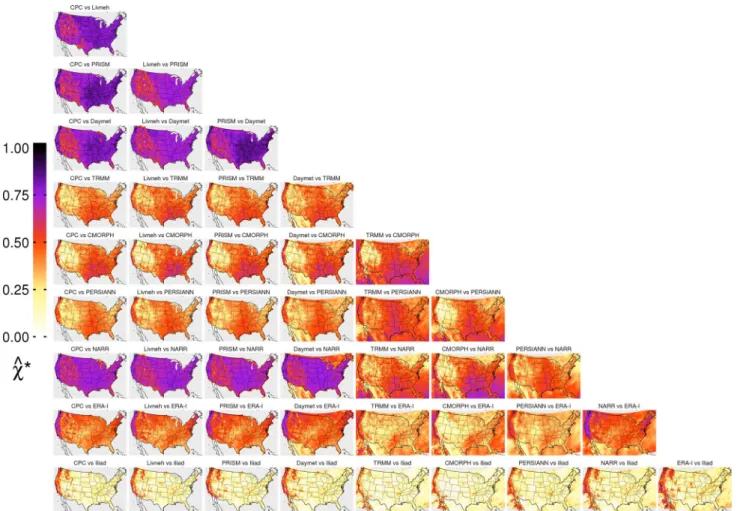
Using the 5-day average, we computed the (Pearson) correlation and 𝜒̂∗ for each pairwise comparison. Findings,

in terms of both spatial pattern of dependence and product relationships are fairly consistent across both analyses so we focus here on results for 𝜒̂∗ , shown in Fig. 6.

Corre-lation analysis for all products is shown in Figure S2 in the supplementary information. The analysis is ordered by rows such that gauge-based products occupy the top three, followed by satellite, reanalysis and finally ILIAD. Note that the exclusion of Maurer here is in part due to it having been “superseded” by Livneh, and partly due to its lack of substantial temporal coincidence with TRMM, CMORPH and ILIAD (2, 2 and 0 years respectively). The gauge-based products show strong extremal dependence with each other, although clearly weaker for the satellite based products, particularly over complex terrain. Of the reanalysis products, NARR exhibits similar qualities to the gauge-based products, such as Livneh, although ERA seems to be consistently lower by ∼ 0.2. In fact,

depend-ence between ERA and TRMM, CMORPH and PER-SIANN appears to be very low, suggesting that the data are asymptotically independent over large areas of the CONUS. The ILIAD simulation output also compares very poorly to most products. The only region showing con-sistently high dependence across all data sets is the west Fig. 4 Correlation between CPC

and Maurer over the CONUS for daily data and 2-, 3- and 5-day averaging windows

coast. This is consistent with the results for correlation and perhaps not surprising given the intense large scale events that dominate precipitation in that region.

The relative strengths of dependence between classes of products are clear from Fig. 6. There is little to distin-guish between the rain gauge products, possibly including NARR, that are based upon many of the same underlying observations. Under close scrutiny however, comparisons with Livneh tend to show a more distinct pattern of disa-greement in regions of elevated and irregular terrain such as the Rocky Mountains. Analysis involving satellite based products, particularly PERSIANN, tends to show smoother spatial features. However, arguably they show more variance in terms of comparisons with each other and with rain gauge products. TRMM and CMORPH for example, exhibit fairly strong dependence in the south east, but show strong conflict in the west, east of Sierra Nevada mountains. CMORPH tends to show the strongest east-west difference in all com-parisons. Of the reanalysis, in general NARR compares more favourably to other products than ERA, particularly for the rain gauge products—likely attributable to the lack of assimilation of gauge observations in ERA.

Inconsistency originating from the treatment of elevated regions and between types of observation platforms are made clear when considering variation between analyses. Figure 7 shows the standard deviation of 𝜒̂∗ computed

from all of the analyses excluding the ILIAD output (Fig. 7a), and only those involving gauge-based products (Fig. 7b). Note that the latter comprises a sample size of six only but serves to highlight the difference between the data types. In particular, the dominant source of variabil-ity in the gauge-based products is on small scale and lies almost entirely over mountainous regions. However, this is small in absolute terms compared with the variance intro-duced by the other products. In a, many regional features are visible, in particular small scale variability in the west and larger scale variability in the east. Individual loca-tions showing high variance can be investigated on a case-by-case basis. For example, the region just west of Salt Lake City (Utah)—the Great Salt Lake Desert—appears to be problematic. At an elevation of 1200 m, the region is fairly flat punctuated with a small number of moun-tains. Annual precipitation is appreciable, ∼ 450 mm per

year for Salt Lake City airport. However, a sparsity of rain Fig. 5 𝜒̂∗ for pairwise comparison of the CPC and Maurer products.

3- and 5-day moving averages are applied in the second and third rows respectively. Analysis based on taking the maximum value

within blocks of 4 × 4 and 10 × 10 native grid cells (at ∼ 25 km) is

gauges in that area, which spans in excess of 10,000 km2 ,

is likely to result in large uncertainties in interpolation that would affect the extremes in particular (Gervais et al.

2014b). The highest value of the standard deviation in that particular region is ∼ 0.175. The values of 𝜒̂∗ for the six

comparisons are in fact clustered into two groups: those compared with CPC and those compared with Livneh. Val-ues for comparisons of CPC with PRISM and Daymet are respectively, 0.63 and 0.65, compared with 0.29 and 0.38 for Livneh. Additionally, values for CPC vs Livneh and

PRISM vs Daymet are 0.35 and 0.67. Livneh appears to be responsible for the majority of the variance, yielding low values of 𝜒̂∗ with each of the other products.

4.3 Seasonality

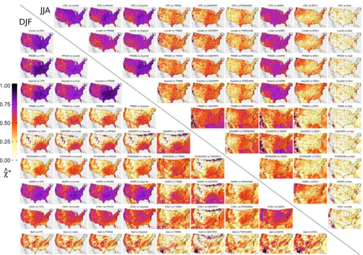
We examined the effect of seasonality on 𝜒̂∗ based on

win-ter (DJF) and summer (JJA) months, shown in the bottom left and top right sections (respectively) of Fig. 8. Sea-sonal decomposition reveals a strengthening of the spatial dependence pattern during DJF, with rather less change Fig. 6 𝜒̂∗ for pairwise comparisons of gridded products after applying a 5-day moving average

Fig. 7 _{Standard deviation of} 𝜒̂∗

for all products (a) and gauge-based products only (b)

during JJA. This appears to reflect the differing strength in seasonal precipitation—the strongest events occur in winter and lower levels of precipitation that occur in sum-mer are separated out. In JJA, the levels and spatial pat-tern of dependence appear to closely resemble the annual analysis (Fig. 6). However, the results for DJF reveal other interesting points. Gauge based products show similarly with annual results, with slightly weaker dependence in the mountains, but comparisons with satellites deterio-rate substantially. They all appear to exhibit zero depend-ence in parts of the northern Rocky Mountains, but for CMORPH in particular, a large proportion of the west has no correspondence with any gauge based product. It turns out that for much of this region and time period CMORPH is zero, which in places results in spurious analysis out-put, visible in Fig. 8 (bottom left) as dark streaks. This arises since only a few non-zero data points exist, and the estimator for 𝜒 is close to one. Xie et al. (2017) describe

the loss of winter time data due to post-processing, which appears to be responsible. For reference, we have included an example analysis from a single grid cell in Figure S3.

It is particularly important to recognise that the seasonal analysis reduces considerably the amount of data available. The ILIAD data set, for example, is reduced to approxi-mately 450 days, and furthermore, depending on region and time period, many of those days may be zeros. Thus the estimation of 𝜒̂∗ is subject to very large uncertainty

(con-ceivably based on only a single event). Note that in areas showing no color, that affect analyses of ILIAD, CMORPH and to a lesser extent some other satellite based products and reanalysis, 𝜒̂∗ took on negative values due to a complete lack

of dependence.

4.4 Temporal non‑stationarity

As discussed briefly in Sect. 3.2, non-stationarity in pre-cipitation time series is the subject of intense research, par-ticularly with respect to extremes in the context of climate change. In some locations in the CONUS extremes may become more intense (Easterling et al. 2017). While such trends are small and essentially irrelevant to our analysis, it is interesting to separate the data record into different time Fig. 8 𝜒̂∗ _{for pairwise comparisons of gridded products during DJF (bottom left) and JJA (top right)}

periods and examine 𝜒 between different products. This also

helps to elucidate other inconsistencies in products, poten-tially due to temporal changes in source observations, grid-ding methodology and other factors.

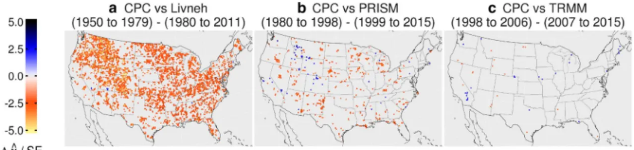
To investigate this issue more fully, we have therefore computed 𝜒̂(q=0.92) for CPC and Livneh for the two

peri-ods, 1950–1979 and 1980–2011. The difference, normalised by its associated standard error, SE_0.92 , is shown in Fig. 9a,

where we have removed data points that exhibit a difference of less than 2 SE_0.92 . For comparison, we have done the same

for CPC vs PRISM (1980–1998, 1999–2011) in b, and CPC vs TRMM (1998–2006, 2007– 2015) in c. In addition we provide Figures S4 and S5 in the supplementary information that show the values of 𝜒̂∗ for the two different time periods,

and absolute differences between 𝜒̂∗ for each decade and the

complete period.

The results show that for CPC vs Livneh, there is a robust decrease in extremal dependence in more recent years for a large part of the CONUS, that is not seen for the other two analyses (b, c). A close inspection of Fig. 9a however suggests that clusters of locations showing the largest differ-ences are constrained by state boundaries in many parts of the CONUS, suggesting that observation timing is again rel-evant and having an effect on extremal dependence. Figure S4 compares 𝜒̂∗ for the various periods, revealing that the

result for the complete period (also seen in Fig. 6) is a little lower than the earlier half (b), and a little higher than the latter half (c). Since, with the exception of CPC vs Livneh, all analyses cover a period after 1979 (or later), Figure S4c (1980–2011) provides a more direct comparison over the recent period. Looking more closely by examining succes-sive decades, Figure S5 reveals that extremal dependence was highest in the 1970s, and, almost without exception, this was systematically higher across the whole CONUS when compared to the 1990s and 2000s. Changes in availability, quality, use and selection of source data may have occurred, and in fact, inspection of Figs. 9a, S4b and S5 readily reveals spatial patterns of extremal dependence that correspond closely to state boundaries. This seems particularly clear

before 1980, and likely related to the timing of observation issues that we identified in Sect. 4.1.

Although a detailed investigation of sources of non-stationarity is beyond the scope of this paper, it appears to be relevant to CPC vs Livneh. It also appears less likely to be relevant to analyses over a shorter period, but a detailed case-by-case investigation would be required to confirm this. Nonetheless, this finding raises further questions as to the reliability of gridded products. Further discussion of Figures S4 and S5 is provided in the supplementary information.

5 Discussion

5.1 Statistical considerations and interpretation.

The application of a metric based upon the tail dependence parameter 𝜒 appears to be a useful tool in this context, that

explicitly quantifies temporal dependence in the extremes. Figures 1 and S1 showed that inference for 𝜒 is not

straight-forward, thus motivating the use of 𝜒̂∗ . However, many

complications remain, and 𝜒̂∗ does not necessarily mitigate

difficulties associated with detecting asymptotic dependence. Importantly, we have yet to make use of uncertainty infor-mation, either directly inferred (see Fig. 1) or from other sources (such as the precipitation products themselves), in evaluating robustness in estimation of 𝜒̂∗ . Nonetheless,

interpretation is important issue.

In the context of our comparative study, 𝜒 appears to

have both valuable qualitative and quantitative interpreta-tion. Qualitatively, for the CONUS for example, we show substantial temporal disagreement between high quality rain gauge and satellite products in many regions, thus if one believes rain gauge products to be the “gold standard”, then this raises many questions about the use of satellites for extremal analysis. This naturally extends to applica-tions where rain gauges are not available, and provides good reasons to question and interrogate satellite derived

Fig. 9 Difference between 𝜒̂(q=0.92₎ normalized by standard error

for pairwise comparisons of gridded products for the first and second halves of their complete duration. CPC vs Livneh, CPC vs PRISM,

CPC vs TRMM are shown in a–c, respectively. Points that exhibit a difference of less than 2 SE0.92 are not shown

data when studying extremes elsewhere around the globe. This is reinforced further given that the CONUS is well studied, and source data and subsequent product devel-opment are likely of the highest available quality. We do nonetheless see levels of disagreement even between gauge based products in mountainous regions. Quantita-tively, Fig. 6 shows 𝜒̂∗∼0.5 in places, implying that the

probability of temporal coincidence of the most extreme events in two products to be no better than a coin flip. This seems like a low level of agreement. For a numeri-cal climate model validation (against observations), this may be regarded as acceptable, given current standards of model development, but for a regional extremal analy-sis of some kind, or even a numerical weather forecast, this might be highly unsatisfactory. In this sense, 𝜒̂∗ can

be used to measure extremal temporal dependence with a reference product in a consistent way. With this in mind, our results appear to raise rather challenging—even awk-ward—questions over the accuracy of “gold standard” gridded products that face a myriad of applications in a leading scientific nation. It is unsurprising therefore that more detailed studies of complex terrain are being under-taken (Henn et al. 2017) and that researchers urge caution when using gridded products (King et al. 2013).

However, the limited extremal differences between cer-tain products in some regions (CPC, Daymet, PRISM), not-ing also very high correlation (Figure S2), may suggest a convergence of gridding methodology and that sources of uncertainty are small. If we believe those to be reference data sets of high accuracy, then this study, having reviewed a wide range of products, provides a comprehensive exposé of which products diverge from the reference, and in which regions. In terms of applications, it seems clear from our results that gridded products must be chosen on a case-by-case basis, but also that many other questions remain, such as those relating to marginal aspects of the product (e.g. magnitude bias, distribution characteristics etc). As an example, possibly relevant to model development, we anticipate that a user could define evaluation criteria based on an absolute value of 𝜒̂∗ , in much the same way as weather

forecast scoring metrics (Ferro and Stephenson 2011). From there, a formal means of testing robustness could also be developed. Nonetheless, given the range of uncertainties and possible applications, we view our results as an indicator of extremal dependence, and encourage their interpretation in terms of relative strengths of dependence between com-parisons. We also add that there can be problems inherent in the analysis of extremes without regard for the complete distribution (Lerch et al. 2017), and we advocate for the use of 𝜒 , and perhaps related scoring measures, as part of any

holistic intercomparison. Ultimately, the question of abso-lute accuracy of any given product is much further reaching, and our analysis serves as a guide to direct enquiry. We make

suggestions as to possible routes for development of this approach at the end of this section.

5.2 Spatial variation of dependence

It is clear from Figs. 6, 8 and S2 that the spatial structure seen in temporal extremal dependence and correlation is fairly consistent throughout the analysis. In general there is a distinction between the eastern and western US, often marked by the edge of the Rocky Mountains, and consist-ently high dependence on the west coast. Seasonally, a more uniform pattern is seen during JJA and more divergence east-to-west is seen during DJF. Both gauge- and satellite-based products tend to more strongly conflict over elevated terrain, which we readily attribute to the challenges of inter-polating station data over complex terrain (Henn et al. 2017), and various issues with inference from satellite radar. Over the CONUS it is well known that rain gauge density is much lower in the western mountainous regions, and that such stations can be substantially affected by location elevation (Groisman and Legates 1994; Daly et al. 2017). Satellites are known to over-estimate the extremes in mountainous areas (Xue et al. 2013; Salio et al. 2015) but they also struggle with cold weather precipitation. (Xie et al. 2017) describe the loss of information due to data quality screening due to snow coverage in winter, and this seems to be commensu-rate with the consistent discrepancy of CMORPH with other products during DJF (see Fig. 8).

In addition to orographic effects, spatial variation of the underlying precipitation processes appears to affect the analysis. ERA and ILIAD, based upon on numerical simulation, appear to struggle with capturing summer time convective precipitation in the midwest, compared with rain gauges. NARR however, assimilates gauge-based observa-tions directly and exhibits dramatically higher dependence in both JJA and DJF. The US west coast stands out some-what uniquely as a region of consistently high agreement in the extremes, although with varying relative strength. It experiences heavy precipitation in DJF, where a few high magnitude seasonal storms due to extratropical cyclones and atmospheric rivers are responsible for almost the entirety of precipitation. In California, this often falls heavily on the Sierra Nevada mountains, which are clearly visible in nearly all panels of Figs. 6 and 8. King et al. (2013) note a similar phenomenon in Southern Australia, where correspondence between a gridded product and reference data is found to be higher on the coast. They speculate that this may be due to the majority of heavy precipitation being due to synoptic scale weather activity. Notable consistency between ERA and ILIAD, and other products suggests that the numerical models do capture large scale precipitation extremes fairly well. ERA also exhibits dependency with gauge-based prod-ucts in the northeast in DJF.

5.3 Product groupings

It is particularly interesting that products fall into fairly well defined groupings that correspond to the sources of obser-vational data (given our choice of color scheme in Figs. 6

and 8). Simply put, the strength of correspondence—both correlation and extremal dependence—is ordered by obser-vation type: rain-gauge, satellite, reanalysis and simulation. This is consistent with the fact that a high quality rain gauge network has lower uncertainty than estimates from satellites, and that data based upon numerical simulation are typically somewhat less accurate and more uncertain still. The four rain gauge-based products are clearly characterized by com-mon source data, but given the range of sources of uncer-tainty in this analysis, including those originating in the raw source data, post-processing and the inference conducted here, it is somewhat surprising that there is so little varia-tion. Figure 7b shows the standard deviation is low (< 0.05) in many locations. However, extremal dependence is not per-fect, 𝜒̂∗∼ 0.8 , implying that some source(s) of uncertainty

may be affecting each product in a fairly consistent way. Variation in interpolation method could be an important consideration. Attribution of dependence characteristics to sources of uncertainty is challenging although some factors are apparent. Satellite derived precipitation suffers from bias in both warm and cold seasons, and reanalysis data appears to be sensitive to which data is assimilated and how it is done.

Regardless, the spread in extremal dependence across all groups of products that we have identified raises important questions about sources of uncertainty and where and when certain products should and should not be used. At the very least, it seems one should be particularly cautious in the absence of a high quality rain gauge network.

5.4 Regridding and product standardization

During this study, we found a remarkable lack of stand-ardization across product format, leading to the need for extensive post-processing that could introduce errors. For example, PRISM and CMORPH are provided only in binary formats, ERA contains (very small) negative precipitation, and while Daymet are available in the more convenient NetCDF format, the former adopts a “standardized” 365 day year (leap days are included but December 31 is dropped from leap years) and the latter lacks a time variable. Geo-graphic grid configurations are almost universally different, dictating the need for a choice of regridding methodol-ogy (of which there are many), and we recognize this as a potentially important source of uncertainty. Choice of grid-ding algorithm may be influential, but re-gridgrid-ding typically smooths out extremal information and inevitably a choice of target resolution is required for direct comparisons, which

might unfavourably affect certain products, including those that require regridding, and those that are processed to a coarser grid. We did not undertake any specific investigation of the impact of (re-)gridding, judging that any introduced uncertainty was no greater than other relevant sources in this case. However, we anticipate addressing this issue more fully in any future studies of this kind. While we acknowl-edge that there are many scientific, practical and historic reasons for disparities in product format and availability, many pitfalls await the researcher who wishes to use multi-ple products (which we advocate). Acknowledging that wide ranging intercomparison studies of this kind are beneficial and necessary, the additional provision of a standardized format (e.g. rectilinear gridded product as monthly NetCDF files) by developers, could bring considerable benefit to users, and alleviate problems and risks of errors potentially introduced through lengthy reformatting processes.

5.5 Further developments

A number of opportunities exist for further development of this approach, including both inference for 𝜒 , the use

of alternative measures and investigation of additional data products. Firstly, we acknowledge that the choice of formu-lation of 𝜒̂∗ is somewhat arbitrary and it may be

advanta-geous to explore alternatives. For example, on closer inspec-tion of Fig. 1f, a negative trend in 𝜒(q)̂ is evident, indicative

of a decreasing level of dependence with quantile. A revised metric that could capture the trend, or other higher order behavior, would be more informative and help mitigate errors arising from point or average estimates. While 𝜒(q)̂ is

based on a non-parametric approach following (Coles et al.

1999), parametric models for extremal dependence struc-ture are available. Our results suggest a range of strength of dependence, from strong asymptotic dependence, particu-larly between gauge-based products, to weakly correlated and likely asymptotically independent data sets. Develop-ment of flexible statistical models that can capture a range of extremal dependence structure is a key area of research in multivariate extreme value theory (see e.g. Ledford and Tawn 1996, 1997), and very much a current focus (Davison and Huser 2015; Huser et al. 2017; Wadsworth et al. 2017). Parametric models like this may provide a more formal framework in which to assess extremal dependence between precipitation data sets, and as such offer a potentially attrac-tive avenue of further investigation.

We noted in Sect. 3.1 that inference for extremal depend-ence is related to scoring statistics that are used, in particu-lar, in weather forecast verification (Jolliffe and Stephen-son 2012; Neiting and Raftery 2007). Alternative scoring measures, that offer different properties than 𝜒 , are proposed

and discussed by Ferro and Stephenson (2011). Although their focus is on weather forecasting, it is clear that there