Development of an adaptive infill criterion for constrained multi-objective asynchronous surrogate-based optimization

(will be inserted by the editor)

Development of an Adaptive Infill Criterion

for Constrained Multi-Objective Asynchronous

Surrogate-Based Optimization

Jolan Wauters · Andy Keane · Joris Degroote

Received: date / Accepted: date

Abstract The use of surrogate modeling techniques to efficiently solve a single objective optimization (SOO) problem has proven its worth in the optimization community. However, industrial problems are often characterized by multiple con-flicting and constrained objectives. Recently, a number of infill criteria have been formulated to solve multi-objective optimization (MOO) problems using surro-gates and to determine the Pareto front. Nonetheless, to accurately resolve the front, a multitude of optimal points must be determined, making MOO problems by nature far more expensive than their SOO counterparts. As of yet, even though access to of high performance computing (HPC) is widely available, little impor-tance has been attributed to batch optimization and asynchronous infill method-ologies, which can further decrease the wall-clock time required to determine the Pareto front with a given resolution. In this paper a novel infill criterion is de-veloped for Generalized Asynchronous Multi-objective constrained Optimization (GAMO), which allows multiple points to be selected for evaluation in an asyn-chronous manner while the balance between design space exploration and objective exploitation is adapted during the optimization process in a simulated annealing like manner and the constraints are taken into account. The method relies on a formulation of the expected improvement for multi-objective optimization, where the improvement is formulated as the Euclidean distance from the Pareto front taken to a higher power. The infill criterion is tested on a series of test cases and proves the effectiveness of the novel scheme.

Conducted as part of the SBO research project 140068 EUFORIA (Efficient Uncertainty quan-tification For Optimization in Robust design of Industrial Applications) under the financial support of the IWT, the Flemish agency of Innovation through Science and Technology. Jolan Wauters, Joris Degroote

Department of Flow, Heat and Combustion Mechanics, Ghent University Sint-Pietersnieuwstraat 41, 9000 Gent, Belgium

Flanders Make, Belgium

E-mail:{jolan.wauters, joris.degroote}@ugent.be Andy Keane

Computational Engineering and Design Group, University of Southampton

Boldrewood Innovation Campus, Burgess Rd, Southampton SO16 7QF, United Kingdom E-mail: [email protected]

Keywords Surrogate Modeling · Kriging · Expected Improvement · Batch Optimization·Multi-Objective Optimization·Constrained Optimization

1 Introduction

With the advent of high performance computing (HPC) it is nowadays possi-ble to model complex systems, such as unmanned aerial vehicles(UAV), turbine cascades and wind farms,using computationally costly simulation codes, such as

computational fluid dynamics(CFD). These complex systems are often character-ized by the absence of a closed form: the problem is given as a black-box which provides an output for a given input. Even though modeling has become feasible, performing the entire design process or even carrying out an optimization on such a system might be an unfeasible problem without the use of a proper framework, even with access to HPC. An established method to handle this kind of prob-lems is the introduction of an intermediate level in the form of a surrogate model, which is constructed using a few well selected evaluations and on which the opti-mization is performed. A well-known surrogate modeling technique is Kriging [11], building forth on the concepts of Gaussian processes and the theorem of Bayes. The stochastic nature of the aforementioned allows the definition of the expected improvement, which can serve as criterion for the selection of the next point to evaluate by balancing design space exploration and objective exploitation [11]. Control over the exploration-to-exploitation ratio during the optimization process can be obtained through the Generalized Expected Improvement [38].

An example of a computationally challenging problem is the optimization of UAVs (or drones). The widespread use of UAVs has become clear over recent years. Within the extensive range of UAVs that exists nowadays, of particular interest are those that operate at a chord-based Reynolds numbers (Rec) below 5×105, the

condition which is referred to aslow Reynolds number flow [29]. During landing, the UAV is characterized by high angles of attack and by the appearance of a large range of frequencies in the flow. This implies that both a small time step size and a large number of time steps is required to correctly resolve the flow and obtain an averaged value of the quantities of interest. As the time steps are solved sequentially, the speed-up by parallelization cannot be increased beyond a certain limit. Optimal use of available computing power is thus obtained by calculating multiple infill points at once. In an attempt to accelerate the optimization pro-cedure by reducing the number of iterations and making full use of parallelized computational power, a multitude of infill points is selected. This can be done in a synchronous manner [32], but with a different convergence rate of the problem in each infill point, a part of the available computing power might be idle, which makes an asynchronous manner more desirable.

Different methodologies exist that tackle the asynchronous selection of mul-tiple design points, which in this case translates itself in finding mulmul-tiple local optima of infill criteria [38]. Gradient-based optimizers in combination with a multi-start or sequential global optimization with the addition of a penalty func-tion in the ‘global’ optimum [37] serve the purpose, but lack the elegance that Gaussian processes have to offer. To complicate matters further, design problems rarely see themselves translated as a single objective optimization (SOO) prob-lem, but rather as a multitude of conflicting demands and thus amulti-objective

optimization (MOO). Since the turn of the century a number of multi-objective formulations of the expected improvement have been formulated which allows a surrogate-based global multi-objective optimization [23, 44, 18, 22, 32, 3].

In this paper we bring together three different concepts: the formulation of the expected improvement for multi-objective optimization, the generalized for-mulation of the expected improvement which allows control over the importance of exploration and exploitation, and the ability to calculate the expected improve-ment in an asynchronous manner. In§2 we present the concept of Kriging followed by an overview of existing infill criteria in§3 and development of novel updating schemes in §4. The concepts are compared and tested on a series of test cases in

§5.

2 Surrogate Modeling: Kriging

Confronted with the staggering computational cost of a single evaluation in certain optimizations, an efficient methodology is sought to find the optimal set of design parametersx= [xi, i= 1, ..., d]. An established methodology to answer the prob-lem at hand is found in the field of surrogate modeling. This implies that, after defining the objective function y(x) and the design space, a design of experiments (DoE) is set up to select n samples in the design space, for which the objective function is subsequently calculated and of which a surrogate is defined. This cheap to evaluate surrogate or meta-model can thereafter be sampled to define the entire characteristics in function of the geometric design variables and can be updated with additional data during the optimization.

The surrogate model used in this work is Kriging, which can be seen as the sum of a trend function and Gaussian process: Y(x) =f(x)Tβ+Z(x) with f(x) = [fi(x), i= 1, ..., m] the vector of basis functions, β the vector of coefficients and

Z(x) a Gaussian processGP(0,cov(y(i),y(j))), with zero mean and fully described by the covariance function cov(y(i),y(j)) =σ2cor(y(i),y(j)), whereσis the process variance and cor(y(i),y(j)) is the correlation function between two designs and is noted for being a function of their inputs and typically written asψ(x(i),x(j)). Here the Mat´ern covariance function is used withν = 3/2which has proven its worth for a number of physical applications [40, 34]. However, it must be emphasized that not every covariance function is equally fitted for every application [45]. The trend is typically the solution of a regression problem and the Gaussian process captures the variation on this trend to exactly interpolate the evaluated data.

In order to determine the parameters of the covariance function, typically referred to as hyperparameters, we maximize the likelihood L that the afore-mentioned surrogate can reproduce the evaluated data. Solving the maximum likelihood estimation (MLE) problem, we can define the Best Linear Unbiased Prediction (BLUP), which allows the prediction of unsampled locations x with respectively the predicted mean and predicted variance:

Y(x) =f(x)Tβ+ψ(x)TΨ−1(y−Fβ) (1) s2(x) =σ2 1−ψ(x)TΨ−1ψ(x) +FTΨ−1ψ(x)−f(x)TFTΨ−1F −1 FTΨ−1ψ(x)−f(x) (2)

with F the n×m model matrix: Fi,j = fi(x(j)) and Ψ the n×n correla-tion matrix:Ψi,j =ψ(x(i),x(j)), ψ(x) = [ψ(x(1),x), .., ψ(x(n),x)] and the MLE of the coefficient vector and the process variance respectively defined by β = (FΨ−1F)−1FTΨ−1yandσ2= _n1(y−Fβ)TΨ−1(y−Fβ).

The construction of the Kriging model is performed using an open source tool-box ooDACE (object-orientated Design and Analysis of Computer Experiments) [4]. The maximization of the concentrated ln-likelihood function is performed through a multi-startsequential quadratic programming (SQP) methodology.

3 Infill Criteria

3.1 Single Objective

The improvement of a predicted point on the current best evaluated point, y_min= min(Y(X)) withX the set of all samples, is defined as (following Janusevskis et

al.’s notation [17]): I(x) = (y_min−Y(x)|Y(_X) =y(_X))+ with (·)+ = max(·,0). The stochastic nature of Kriging allows the assessment of the uncertainty in the prediction. This can be used to define the expected improvementE[I(x)] =EI(x)

[27]: EI(x) = Z ∞ −∞ I(Y)φ(Y,x)dY = Z ymin −∞ (ymin− Y) 1 s(x)√2πexp −(Y −Y(x)) 2 2s2_(x) dY. (3)

This leads to the well-known formula of the expected improvement,

EI(x) =

(

(ymin−Y(x))Φ(u(x)) +s(x)φ(u(x)) ifs >0

0 otherwise (4)

with Φandφrespectively the standard normal cumulative and probability den-sity function, φ the one-dimensional Gaussian probability density function and

u(x) = (ymin−Y(x))/s(x). Note that the first term drives the minimization of the objective (exploitation), while the second term drives the minimization of the uncertainty of the prediction (exploration). Alternatively, the expected improve-ment can be formulated as

EI(x) = yminΦ(u(x))− Z ymin −∞ Yφ(Y,x)dY = ymin− Rymin −∞ Yφ(Y,x)dY Φ(u(x)) ! Φ(u(x)) = ymin−CP[(x)] P [(x)]. (5)

This allows a geometrical interpretation of the expected improvement: the product of the area under the probability density function cut off by the best evaluation (P[I(x)]) and the distance between the centroid of the aforementioned area and the best evaluation|ymin,CP[I(x)]|(figure 1) [43].

|ymin,CP[I(x)]|

Fig. 1: Graphical interpretation of the expected improvement, corresponding to the product of the probability of improvenent P[I(x)] and the distance of its centroid to the current best evaluation |ymin,CP[I(x)]|. Reproduced from Forrester et al.

[11]

Algorithm 1Efficient Global Optimization (EGO) [20] Require: Evaluated sampling plan (X,y(X))

Ensure: The best observation (xmin,ymin) 1: whilestopping criteria are not metdo

2: Estimate hyperparameters .Section 2

3: xnew= arg maxxEI(x) .Equation 4

4: X←X∪xnew 5: ymin←minx(y(X)) 6: xmin←arg minx(y(X))

This infill criterion forms the basis of the well known efficient global optimiza-tion (EGO) algorithm by Jones et al. [20] (see Algorithm 1). However, based on

the observation that Kriging is prone to an underestimation of the prediction er-rors caused by the assumption of a fully known parameter and hyperparameter set, the expected improvement is prone to higher emphasis on the estimated value [38]. Especially at earlier stages of the optimization, this may lead to the infill cri-terion getting stuck in a possibly local optimum and overemphasizing the region before exploring the parameter space further. To counter this phenomenon, Schon-lau et al. [38] proposed a generalized formulation of the improvement by taking it to a higher power, effectively deriving the generalized expected improvement

E[Ig(x)] =GEIg(x) GEIg(x) =sg g X k=0 (−1)k g k ! u(x)g−kTk (6) withTka recursive function given byTk=−uk−1φ(u)+(k−1)Tk−2withT0=Φ(u)

andT1 =−φ(u) and u = (ymin−Y(x))/s(x). Sasena et al. proposed to haveg decrease in a ‘Simulated Annealing’-like manner with the objective of attributing more importance to objective space exploration early in the optimization and more importance to objective exploitation later on [36]. Table 1 shows the value of g

during the optimization as proposed by Sasena et al.

Table 1: Sasena et al.’s cooling scheme [36]

Iteration 1-4 5-9 10-19 20-24 25-34 ≥35

g-value 20 10 5 2 1 0

In case that more computing nodes are available than the number of nodes over which a single evaluation of the objective function can be spread, it becomes worthwhile to determine multiple infill points at once in a synchronous or asyn-chronous manner.

Examples of existing synchronous methods are amongst others the Clustered Multiple Generalized Expected Improvement(CMGEI), which uses the generalized formulation of the expected improvement and was proposed by Ponweiser et al. [32]. In their work they cluster based on the Mahalanobis distance to select a multitude of points to be evaluated simultaneously. A similar approach is brought forward by S´obester et al. [37], which relies on a multitude of local optima of the EI criterion. Ginsbourger et al. [14] came up with the q-steps EI, in which the design space is enhanced q-fold such that the q-steps EI optimum corresponds to q optimal points to be filled in simultaneously. An analytical expression was formulated by Chevalier [1] relying on Tallis’ formula. An expression of the gradient was subsequently derived by Marmin et al. [25].

In case of an asynchronous setting, a straightforward approach is the use of penalty functions. Schonlau et al. [38] proposed asequential design in stageswhere the global optimum of the expected improvement is sought and subsequently the model’s prediction is added to the training set. After retraining the model, the variance reduces locally to zero and repeating the procedure ensures that the next infill point moves away from previously added samples. While use is made of the stochastic nature of the surrogate model, this method relies on the assumption that the predictor is accurate enough. Ginsbourger et al. referred to this method as

Kriging Believer(KB) and alternatively proposed aConstant Liar(CL) approach [14]. Furthermore, the addition of an infill point and the accompanied retraining of the model can be computationally costly. More accurate is the calculation of the expectation of the EI (EEI [13]). However, since there is no tractable analytical expression of the aforementioned, this is typically calculated using Monte Carlo Integration (MCI), maintaining its expensive nature. All of the aforementioned methods have a sequential approach and are thus in essence asynchronous updating methods. This may become prohibitive, up to the point that not all the computing nodes get filled up because the calculation of a new infill point might exceed its evaluation.

Janusevskis et al. [16, 17] defined the asynchronous multi-points expected im-provementEI(µ,λ) when µ computing nodes are evaluating the objective and λ

computing nodes are available to be filled, allowing the aforementioned methods to be grouped:

EI(µ,λ)(Xλ) =E[min(Y(X∪Xµ))−min(Y(Xλ))|Y(X) =y] (7)

withXµ =x(1)_b , ...,x(_bµ)the set of parameter combinations that is currently being evaluated andXλ =x

(1)

a , ...,x(aλ) the set of parameter combinations that is to be determined for evaluation. Ifµ= 0 andλ= 1 we obtain the well knownEI. In case thatµ= 0 and λ≥ 2 we obtain the earlier describedq-steps EI. Janusevskis et al.’s [16, 17] proposed a mixed strategy to determine the most promising batch by combining MCI with bounds to allow ranking of candidate points, thus reducing the number of samples required. Here, we present a reformulation of the MCI of

q−EI(as introduced in [14]) forEI(µ,λ)(see algorithm 2). The method relies on the numerical integration of the multivariate distribution of the µ+λunknown responses conditional on the observations Y(Xµ+λ) ∼ N(Y(Xµ+λ),Ψµ+λ) with Xµ+λ= [Xµ,Xλ]T and

Ψ_µ(i,j_+λ)=ψ(X(µi+)λ,X (j)

µ+λ |Y(X) =y) where i, j = 1, ..., µ+λ. (8) Consequently, the law of large numbers (LLN) gives us

I_sim(µ,λ)(i) = [min(y,Mµ(i))−min(Mλ(i))]+ (9)

EI(µ,λ)(Xλ) = lim nsim→∞ 1 nsim nsim X i=1 I_sim(µ,λ)(i) (10)

with nsim the number of random sampling sets, Mµ+λ(i) = [Mµ(i),Mλ(i)]T a (µ+λ)×1 vector and a random sampling of Y(_Xµ+λ) obtained through Kaiser & Dickman’s method, which is a straightforward procedure relying on the con-cepts of Principal Component Analysis (PCA) [21]. PCA states that a sample matrix Z from a multivariate normal distribution specified by the correlation matrix Ψµ+λ can be obtained from a linear transformation of a set of indepen-dent, identically distributed univariatesN ∼ N(0µ+λ,Iµ+λ) through Z=L·N with L the Cholesky decomposition of the covariance matrix L = chol(Ψµ+λ), such that Ψµ+λ = L·LT. This leads to the following results for the sampling:

Mµ+λ=Y(Xµ+λ) +L·N. A more extensive overview of the sampling of a

mul-tivariate normal distribution using a decomposition of its covariance matrix and alternative methods is given in [12].

Algorithm 2Asynchronous Multi-Points Expected Improvement (EI_{M C}(µ,λ))

1: ConstructΨµ+λ .Equation 8

2: L= chol(Ψµ+λ) .Cholesky decomposition of covariance matrix

3: fori←1, nsimdo .Loop over simulation size

4: N(i)∼ N(0µ+λ,Iµ+λ) .Sample from i.i.d. univarites 5: Mµ+λ(i) =Y(Xµ+λ) +L·N(i) .Kaiser & Dickman’s method

6: [Mµ(i),Mλ(i)]T=Mµ+λ(i)

7: I_sim(µ,λ)(i) = [min(y,Mµ(i))−min(Mλ(i))]+ _{.Equation 9} 8: EI_{M C}(µ,λ)=_n1 sim Pnsim i=1 I (µ,λ) sim (i) .Equation 10 3.2 Multi-Objective

When dealing with a design problem, engineers are often confronted with conflict-ing objectives. This issue can be resolved by creatconflict-ing a sconflict-ingle objective function which is made up out of a weighted sum of the different objectives. However, this only moves the problem further downstream: what weight is attributed to which objective? An alternative is to determine the (hyper-)surface of non-dominated ob-jectives for which we cannot improve on one without deteriorating on the other(s). This surface is typically referred to as the Pareto front [9]. During the 90s a num-ber of multi-objective evolutionary algorithms (MOEAs) were proposed to solve this issue, amongst others Fonseca and Flemings’s MOGA [8], Srinivas and Deb’s NSGA [39], Horn et al.’s NPGA [15], Zitzler and Thiele’s SPEA [50], Knowles and Corne’s PAES [24] and at its pinnacle Deb et al.’s NSGA-II [5], to name but a few. While many of these algorithms have proven their abilities, their stochastic nature leads to a very high computational cost if the objectives are expensive to evaluate.

A solution of the aforementioned is the introduction of an intermediate sur-rogate to overcome the prohibitive computational cost of MOEAs [42]. Inspired by the EGO algorithm, the turn of the century has seen the birth of a series of multi-objective reformulations of the expected improvement. One of the earlier approaches, ParEGO [23], reformulates the multi-objective problem as a single objective problem using an augmented Tchebycheff function. A generalization of this approach, MOEA/D (Multi Objective Evolutionary Algorithm based on De-composition) was presented by Zhang et al. [44] and allows a level of parallelization through the formulation of a series of single-objective optimization subproblems. The generation of the Pareto front is in these approaches subjected to the weighting function. Especially in case of nonconvex Pareto fronts this may lead to clustering of evaluations in the extremes of the front and a poor resolution and spread of the region in between. Jeong & Obayashi’s Multi-EGO [18] uses a multi-objective genetic algorithm to determine the Pareto front of the EIs of both objectives and selects three points on the front (both extremes and a point in the middle) as infills for the next iteration, thus enforcing a level on parallelization in the algorithm. Keane [22] presented a formulation of the expected improvement for two objectives based on the geometrical interpretation of the EI (Wagner et al. refer to this as the Euclid-EI [43]). Emmerich et al.’s SExI (S-metric Expected Improvement) al-gorithm [7], Ponweiser et al.’s SMS (S-Metric Selecting)-EGO algorithm [32] and Couckuyt et al.’s EMO (Efficient Multi-objective Optimization) algorithm [3] use the hypervolume (HV) orS-metric, which corresponds to the Lebesque measure

of the hyperspace dominated by the Pareto front. A strong theoretical assessment of the aforementioned can be found in Wagner et al. [43].

In this paper we start from Keane’s formulation, which we briefly summarize here. For a SOO problem, the EI can be understood as the product of the area under the tail of the prediction cut off by the best evaluation and the distance between the centroid of the aforementioned area and the best evaluation [43]. For two objectives Keane reformulates this as the product of the probability that a prediction is found outside the Pareto front,P[I(x)], with the Euclidean distance of the nearest point on the Pareto front, y₁∗_,2 ={[y₁∗(1),y∗₂(1)], ...,[y∗₁(m),y∗₂(m)]}, with m the number of points on the Pareto front, to the centroid of the area outside the Pareto front, ( ¯Y1(x),Y¯2(x)):

E[I(x)] =P[I(x)] q ¯ Y1(x)−y∗1 2 + Y¯2(x)−y∗2 2 (11)

In this work, building forth on the assumption of uncorrelated objectives, a two-dimensional Gaussian probability density functionφ(Y1,Y2,x) for the predicted

responses is constructed φ(Y1,Y2,x) = 1 s1(x) √ 2πexp −(Y1−Y1(x)) 2 2s2 1(x) · 1 s2(x) √ 2πexp −(Y2−Y2(x)) 2 2s2 2(x) (12)

By integrating this two dimensional Gaussian probability density function over the region outside the Pareto front1 we obtain the multi-objective probability of improvementP[I(x)] =P[Y1(x)<y∗1∩ Y2(x)<y∗2]. P[I(x)] = Z y∗(1)1 −∞ Z ∞ −∞ φ(Y1,Y2,x)dY2dY1 + m−1 X i=1 Z y∗(i+1)1 y∗(i)1 Z y∗(i+1)2 −∞ φ(Y1,Y2,x)dY2dY1 + Z ∞ y∗(m)1 Z y∗(m)2 −∞ φ(Y1,Y2,x)dY2dY1 (13)

The first, second and third term in equation 13 correspond to respectively the series of blocks I, II and III as presented in figure 2. The calculation of the centroid

¯

Y1(x) is performed by determining the first moment of area and dividing it by the

multi-objective probability of improvement:

1 _{Depending on whether it is the intent to improve upon the existing Pareto front (figure 2,} hatched area) or refine the existing front (figure 2, gray area), the limits of the integrals are slightly different. Here, improvement upon the Pareto is presented. For further details on this matter, see [22].

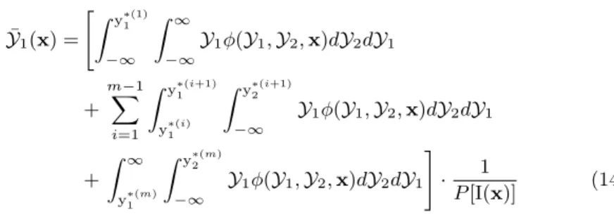
¯ Y1(x) = " Z y∗(1)1 −∞ Z ∞ −∞ Y1φ(Y1,Y2,x)dY2dY1 + m−1 X i=1 Z y∗(i+1)1 y∗(i)1 Z y∗(i+1)2 −∞ Y1φ(Y1,Y2,x)dY2dY1 + Z ∞ y∗(m)1 Z y∗(m)2 −∞ Y1φ(Y1,Y2,x)dY2dY1 # · 1 P[I(x)] (14) ¯

Y2(x) is calculated in an analogous way.

y1(x) y2(x) I II II II III (y∗1(1),y ∗(1) 2 ) (y∗₁(2),y∗₂(2)) (y∗₁(...),y∗₂(...)) (y∗₁(m),y∗₂(m)) •( ¯Y1(x),Y¯2(x))

Fig. 2: Schematic representation of the partitioning of the area outside of the Pareto front of two contesting objectives. The hatched area corresponds to the area where the Pareto front can be improved. The grey area corresponds to the area where the Pareto front can be refined. Reproduced from Keane [22].

4 New Infill Criterion

A limitation of Keane’s EI is the absence of a clear formulation of the improve-ment [43]. This is related to the geometric origin of the way by which it is built up and the intrinsic difficulty of the multidimensional untractable inte-gral that comes with it. Therefore we formulate the improvement (correspond-ing to the utility function in the field of rational decision theory)as the distance from the Pareto front taken to a power g: Ig(x) = [|Pareto(Y(X)),Y(x)|g]+min. Here |Pareto(Y(X)),Y(x)| is defined as the distance measured from the Pareto

front to Y(x) and [·]+_min is defined as the smallest value evaluated outside of the Pareto front. To facilitate the expanation, the equations will be limited to

two objectives in the following step. For two objectives2, this corresponds with Ig(x) = [(p

(y∗

1−Y1(x))2+ (y∗2−Y2(x))2)g]+min. If g is an even number (with

h=g/2), the formulation simplifies due to the disappearance of the square root. This leads to a tractable definition of the expected improvement E[Ig(x)], to

which we refer as the generalized Euclidean/Multi-objective Expected Improve-ment (GMOEI). By making use of the binomial theorem3, we obtain

E[Ig(x)] =E " _h X k=0 h k ! (y∗₁−Y1(x))2k(y∗2−Y2(x))2(h−k) # . (15)

This can be rewritten under the assumption that the objectives are uncorrelated.

E[Ig(x)] =E h (y∗₁−Y1(x))2n i + h−1 X k=1 h k ! E h (y∗₁−Y1(x))2k i ·_Eh(y∗2−Y2(x))2(h−k) i +E h (y∗2−Y2(x))2n i (16)

By partitioning the integrand space in boxes as was done by Keane and is presented in figure 2,E(y∗1−Y1(x))2kcan be rewritten as

E h (y∗₁−Y1(x))2k i = Z y∗(1)1 −∞ Z ∞ −∞ (y₁∗(1)− Y1(x))2kφ(Y1,Y2,x)dY2dY1 + m−1 X i=1 Z y∗(i+1)1 y∗(i)1 Z y∗(i+1)2 −∞ (y₁∗(i)− Y1(x))2kφ(Y1,Y2,x)dY2dY1 + Z ∞ y∗(m)1 Z y∗(m)2 −∞ (y∗₁(m)− Y1(x))2kφ(Y1,Y2,x)dY2dY1. (17) Analogously forE(y∗2−Y2(x))2k

. The result of equation 17 is given by

E h (y∗₁−Y1(x))2k i =E h (y∗₁(1)−Y1(x))2k i + m−1 X i=1 E h (y∗₁(i+1)−Y1(x))2k i −_Eh(y₁∗(i)−Y1(x))2k i Φ y ∗(i+1) 2 −Y2(x) s2(x) ! +E h (y∗1(m)−Y1(x))2k i Φ y ∗(m) 2 −Y2(x) s2(x) ! (18)

2 _{Theoretically the method can be rewritten for any number of objectives. However this} method, as any other, is subjected to the curse of dimensionality (no-free-lunch theorem). In practice, defining the computational domain outside the Pareto front for more than two objectives can be become cumbersome [4] and is for most methods the limiting factor in their applicability.

where_E[(y∗₁(i)−Y1(x))2k] can be calculated using equation 6. With a higher value

of g, a larger size of the current Pareto front and a larger number of infills, the recursive formulation can become cumbersome, up to the point that a simple Monte Carlo approach can become more feasible.

In a similar manner to the single objective case, the asynchronous multi-points GMOEI can be formulated.

GM OEI(g,µ,λ)(Xλ) =E[|Pareto(Y(X∪Xµ)),Y(Xλ)|Y(X) =y|g]+min (19) However, as its SOO variant, the analytical expression becomes challenging, leading us to again resort to numerical multivariate integral approximation tech-niques in the form of Monte Carlo Integration (MCI).

I_sim(g,µ,λ)(i) =|Pareto(y,Mobj,µ(i)),Mobj,λ(i)|gmin (20)

GM OEI_{M C}(g,µ,λ)(Xλ) = 1 nsim nsim X i=1 I_sim(g,µ,λ)(i) (21)

The multivariate sampling of each objective {M_λ(j₊)_µ(i)}j=1...nobj (with nobj the number of objectives) is performed as in algorithm 2 using Kaiser & Dickman’s method.

If (g, µ, λ) corresponds to (1,0,1) we obtain a variant4 of Keane’s EI. When (g, µ, λ) corresponds to (1,0,2) we obtain a multi-objective formulation of the

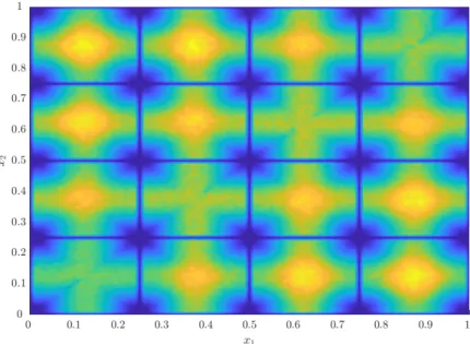
q−steps EI. In the case of a single variable problem, the latter can be visualized as in figure 3. It can be seen that the figure is symmetric around its diagonal, which corresponds to (1,0,1)5with local minima at 0, 0.25, 0.5, 0.75 and 1, where the function has been evaluated and local maxima in between these points. Com-bination of these local optima on the diagonal create the global hot spots. While the local maxima on the diagonal are near equal in value, the hot spots become brighter when moving towards the top left (or bottom right), which indicates that distance between the sampled points is taken into account. Methods relying on lo-cal optima for batch optimization will fail when only one optimum exists. However, this method will select a multitude of points around the optimum at a distance from each other [14].

4 _{Keane’s formulation is characterized by the absence of a definition of the improvement, but} the presence of an analytical form of the expected improvement, which relies on the calculation of the centroid of the prediction outside the Pareto front and determining the distance to the nearest point on the front. Here the improvement is analytically defined as the Euclidean distance from the front. However, this leads to the absence of an analytical formulation of the expected improvement, unless the improvement is taken to an even power, as seen above. The calculation of the improvement relies on MCI where the distance of each sample is taken to the nearest point on the front.

5 _{The addition of a point leads to a reduction of the improvement that can be made at} the point to zero, thusGM OEI(1,0,2)_(x

1,x2) =GM OEI(1,0,1)(x1) =GM OEI(1,0,1)(x2) if

Fig. 3: Contour plot colored by GM OEI(1,0,2) as a function of two infill points (x1, x2) for a simple one variable problem (min y1(x) = (10x−10)2 andy2(x) =

(10x−12)2) after five equally spaced fill-ins, namelyx= 0,0.25,0.50,0.75 and 1.

When dealing with a constrained optimization problem,EIshould decrease to zero when the constraint is violated. This can be obtained through an extended ex-pected improvement [38] or a penalty function, such as the Augmented Lagrangian function [2]. Here, the former is used: given the surrogate of the constraintGwith

G(X) =g, we can calculate the probability of the prediction not violating the

con-straint limitgmin, i.e. the probability that the constraint is met,P[F(x)], where

F is the measure offeasibility G(x)−gmin. Under the assumption of uncorrelated objectives and constraints, it is easy to reformulate the expected improvement such that it accounts for the probability of feasibilityE[I(x)∩F(x)] =E[I(x)]P[F(x)].

This implies that at a given point in the design space, while the predicted con-straints might be violated, the predicted errors in the constraint models are dif-ferent from zero and as such the expectation of feasible improvement will be low, but not zero, since there is a finite possibility that a full evaluation of the con-straints may actually reveal a feasible design. This allows design space exploration in the early stages of the optimization methodology, but ensures convergence to the exact constrained optimum [11]. Nevertheless, Parr et al. remark that if the constraints are approximated inaccurately early on, the algorithm may discard optimal solutions [31].

The inclusion of the probability of feasibility of the constraint(s) in a sampling-based evaluation of the expected improvement corresponds to the multiplication of the aforementioned with the numerical integration (through sampling) of the heaviside function evaluationHof these samples drawn from the multivariate

dis-tribution of the constraintsG−gmin. It is further on assumed thatGis formulated such thatgmin= 0.

F_sim(k)(i) = λ Y l=1 H{M_con,λ(k) (i)}l (22) GM OEI_{c,M C}(g,µ,λ)= 1 nsim nsim X i=1 I_sim(g,µ,λ)(i) ncon Y k=1 1 nsim nsim X i=1 F_sim(k)(i) ! (23)

The multivariate sampling of each objective{M_obj,λ(j) _+µ(i)}j=1...nobjand each con-straint {M_con,λ(k) _+µ(i)}k=1...ncon (with ncon the number of constraints) is again performed as in algorithm 2 using Kaiser & Dickman’s method. The feasibility of each constraint corresponds to the product of the Heaviside evaluations of each element of the sampling of the multivariate distribution of the available computing nodes to be filled.

Algorithm 3 Generalized Asynchronous Constrained Multi-Objective Expected ImprovementGM OEI_{c,M C}(g,µ,λ)

1: forj←1, nobjdo .Loop over objectives

2: L(j)_obj= chol(Ψj[Xµ+λ|Yj(X)≡yj])

3: fork←1, ncondo .Loop over constraints

4: L(k)con= chol(Ψk[Xµ+λ|Gk(X)≡gk])

5: fori←1, nsimdo .Loop over simulation size

6: N(i)∼ N(0µ+λ,Iµ+λ) .Sample from i.i.d. univarites 7: forj←1, nobj do

8: M_obj,µ+λ(j) (i) =Yj(Xµ+λ) +L(j)obj·N(i) .Kaiser & Dickman’s method 9: I_sim(g,µ,λ)(i) =|Pareto(y,Mobj,µ(i)),Mobj,λ(i)|g_min .Equation 20 10: fork←1, ncon do

11: M_con,µ+λ(k) (i) =Gk(Xµ+λ) +L

(k)

con·N(i) .Kaiser & Dickman’s method 12: F_sim(k)(i) =Qλ l=1H({M (k) con,λ}l(i)) .Equation 22 13: GM OEI_{c,M C}(g,µ,λ)(Xλ) =_n1 sim Pnsim i=1 I (g,µ,λ) sim (i)· Qncon k=1( 1 nsim Pnsim i=1 F (k) sim(i)) .Equation 23 5 Results

A comparative study is set up from the perspective that we have a fixed compu-tational budget and a large number of computation nodes, but are limited in the parallelization of each computer experiment and therefore must resort to batch op-timization to make full use of the computational power available. Furthermore, it is assumed that the generation of the next infill is negligible compared to the com-putational cost of its evaluation. The GAMO algorithm (algorithm 4) is used em-ploying six different settings of (g, µ, λ), namely (1,0,1), which resembles Keane’s EI, (1,0,2), which resembles a multi-objective formulation of the q−steps EI,

(1,1,1), which resembles an asynchronous formulation of Keane’s EI, and a gen-eralized formulation of the three aforementioned withgdecreasing in a simulated annealing way as will be explained further, sog=f(l), withlthe current iteration number. For the DoE we use a Latin-Hypercube Sampling (LHS) approach [26] and Morris and Mitchell’s maximin-criterion to quantify the space-filling property by maximizing in ascending order the distance between pairs of points and simul-taneously minimizing the number of corresponding pairs [28]. The stopping criteria used corresponds to a maximum of 100 function evaluations after the DoE or if the normalized expected improvement drops below 0.1%. This means (1,0,2), (f,0,2) perform a maximum of 50 iterations, while the other infill criteria stop after a max-imum 100 iterations. Alternatively, the wall clock time could be set as a stopping criterion, in which case, under the assumptions above, (1,0,2), (f,0,2), (1,1,1) and (f,1,1) would be able to evaluate twice as much simulations as (1,0,1) and (f,0,1). Both criteria are probable to occur in industry, but here we have chosen the former because it allows the assessment of the performance of the infill criteria for a near similar number of evaluations. Furthermore, the selection of a new infill point, especially later in the optimization process at which point the generation of the surrogate model and the sampling of the surrogate become computationally more demanding, can become non-negligible in comparison to the evaluation of a sample. At this point, the asynchronous approaches (1,1,1) and (f,1,1) will outperform the synchronous approaches (1,0,2) and (f,0,2).

Algorithm 4Generalized Asynchronous Multi-objective Optimization (GAMO) Require: Evaluated sampling plan (X,y(X))

Ensure: The Pareto front (x∗,y∗_1,2) 1: whilestopping criteria are not metdo

2: λ≡n({completed(Y(X(i)µ )}i=1...µ) .Determine number of available nodes 3: Xc←Xµ:{completed(Y(X(i)µ )}i=1...µ

4: X←X∪Xc

5: Estimate hyperparameters for every objective/constraint .Section 2 6: y∗

1,2←Pareto(y(X)) 7: x∗_{←argPareto(y(}

X)) 8: Xµ←Xµ\Xc

9: µ≡n(Xµ) .Determine number of calculating nodes 10: Xλ= argmaxxGM OEI

(g(l),µ,λ)

c,M C (x) .Algorithm 3

11: Xµ←Xλ∪Xµ 12: µ≡n(Xµ)

13: l←l+ 1 .Update iteration counter (table 2)

We adopt here a different cooling function than Sasena et al. [36] (table 2) based on the observation that decreasing the power of the improvement to zero, which corresponds to the multi-objective probability of improvement [46, 47], can lead to a stagnation of the optimization process in the form of clustering. Therefore, we spread out the change of power over a larger number of iterations and let it decrease to 1, which corresponds to the first case. By no means can it be expected that the cooling scheme proves to be effective in every case, nor can it be stated that it corresponds to the best performing scheme on a broader average sense, but we expect that placing the emphasis on exploration rather than exploitation early on in the optimization algorithm can accelerate its convergence.

Table 2: Modified cooling scheme based on Sasena et al. [36]

Iteration 1-4 5-9 10-24 25-49 ≥50

g-value 20 10 5 2 1

The methodology is tested on a total of six test functions. The first five test functions are taken from Zitzler et al. [48] (referred to as ZDT1, ZDT2, ZDT3, ZDT4 and ZDT6) and have a particular feature that causes convergence issues for MOO: convexity, non-convexity, discrete Pareto front, multimodality and biased search spaces. All of these have been rewritten in the appendix for six parameters to ensure a certain level of complexity, without using the surrogate outside of its typical application: Kriging is known to have performance issues when dealing with more than 15 parameters or 500 infills [22].A unifying overview of methods that at-tempt to overcome these limitations is amongst other given by Quinonero-Candela and Rasmussen [33].The sixth test function, Osyczka & Kundu’s constrained test problem [30] (abbreviated as OSY), has six parameters and six constraints, all of which are active on different parts of the Pareto front. The solutions and formulas of the aforementioned are given in the appendix. Conform Jones et al’s suggestion, a DoE-size of 65 samples is selected [20].

In their theoretical assessment of performance metrics for multi-objective opti-mization Zitzler et al. [49] state that performance refers to both quality of outcome and the computational resources needed to generate that outcome. Where the per-formance of a SOO solving algorithm can be assessed by measuring the difference between the exact minimum and the predicted minimum in function of number of iterations, the MOO case is more complex due to its competing nature: on the one hand we want to assess the closeness to the optimal front solutions and on the other hand we want to assess the coverage of the front. Furthermore, we want both to be obtained with the smallest computational budget possible. However, coverage of the front can only improve further with additional computational re-sources. Therefore, performance of MOO algorithms cannot be measured with a single metric as pointed out by Van Veldhuizen & Lamont [41]. Riquelme et al. [35] report over 50 metrics used to assess the performance of evolutionary multi-objective optimization (EMO) algorithms of which the hypervolume metric is the most used. Deb et al. [5] presented two metrics to assess the performance: the convergence metricγ, which measures the mean distance of the evaluated Pareto front to the exact one,

¯ γ= 1 m m X i=1 γi (24) γi= min r yp₁−y₁∗(i)2+yp₂−y₂∗(i)2 (25)

with (yp₁,yp₂) the exact Pareto front, and the diversity metric∆, defined as ∆= df+dl+ Pm−1 i=1 |di−d¯| df+dl+ (m−1) ¯d (26) di= r y₁∗(i)−y∗₁(i+1)2+y∗₂(i)−y₂∗(i+1)2 (27) df = r ymin 1 −y ∗(1) 1 2 + y2(x|y1(x) =ymin₁ )−y∗₂(1) 2 (28) dl= r y1(x|y2(x) =ymin2 )−y ∗(m) 1 2 +ymin 2 −y ∗(m) 2 2 (29) ¯ d= 1 m−1 m−1 X i=1 di (30)

wheremis the number of points on the front,diis the Euclidean distance between two consecutive points on the front and ¯dits average. Furthermore,df anddl rep-resent the Euclidean distances between the extreme solutions and the boundary solutions of the obtained non-dominated set. The convergence metric is reformu-lated to determine the correctness of the surrogate around the Pareto front. Even when we run out of computational resources, the cheap to evaluate surrogate can be sampled to refine the regions of the Pareto front which are of particular interest. The convergence metric is defined here as the mean distance between 100 points on the exact Pareto front and their corresponding predicted points. This metric is normalized by dividing it by the largest distance in the objective space. As such ¯

γnorm = 0 corresponds with a perfectly predicted Pareto front. Furthermore, ¯γ (the subscript will from now on be omitted for clarity) can be bigger than 1, when the predicted objective space is larger than the exact objective space. Similarly,

∆= 0 corresponds to a perfectly spread evaluated Pareto front where the extrem-ities of the front are found. Again,∆ can be larger than 1. It can be noted that with as little as three points∆can be zero (the extremities and a point exactly in the middle) and with ¯γnormequal to zero, the surrogate predicts the Pareto front perfectly. However, this is by no means an optimal solution. Therefore, the hyper-volume of the non-dominated objective space is added as another metric with its reference point at the border of the objective space and normalized by dividing it by the area of the entire objective space.

y1(x) y₂(x)

Pareto front 1st_run Pareto front 2nd_run Pareto front 3rdrun Pareto front 4th_run Pareto front 5th_run

best summary attainment surface median summary attainment surface worst summary attainment surface

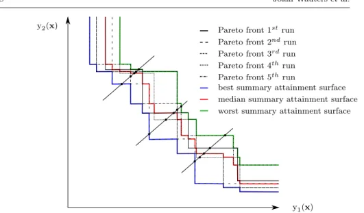
Fig. 4: Schematic representation of the Pareto fronts of five independent runs of an optimizer with three diagonal lines intersecting the aforementioned fronts which allow the formation of thep-summary attainment surfaces, with the 1st, 3rd and 5th summary attainment surfaces respectively corresponding to the best, median and worst surfaces. Reproduced from Knowles [23].

The stochastic nature of the optimization caused by the randomly generated DoE can lead to a varying performance. To take this aspect into account, the optimization is repeated 10 times and the average and variance of ¯γnormand∆are determined. Furthermore, thep-summary attainment surfaces are determined, of which the best, median and worst hypervolumes are calculated following Knowles in his analysis of the ParEGO algorithm [23]. Givennruns of the algorithm, the obtained attainment surfaces/Pareto fronts6can be plotted on top of each other. If a diagonal, running in the direction of the improvement in all objectives, is drawn through this set of fronts, it can be stated that the intersections, n in total, lie on their respective summary attainment surface. The best summary attainment surface thus corresponds to the attainment surface formed by the Pareto optimal points on the intersecting diagonals. If we then remove the points that make up the best summary attainment surface and select the Pareto optimal set of the remaining points, we obtain the 2nd-summary surface and so on. We emphasize three of these summary attainment surfaces from a statistical point of view: the best, which corresponds to the best front the algorithm can hope to produce, the worst, which corresponds to the best attainable surface that will be dominated during every run of the algorithm, and the median, which corresponds to the performance that can be expected half of the time. The concept is visualized in figure 4. The hypervolume of the three aforementioned summary attainment surfacesSpis calculated as the final metric to assess convergence and the reference point is placed at the border of the objective space. This metric is rewritten such

6 _{The attainment surface was formally defined by Fonseca & Fleming and corresponds to} the Pareto front [10]. Both terms are interchangeably used in the optimization community, but in the context of metrics the former is preferred.

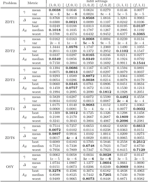
Table 3: Results of GAMO for different infill settings and different test functions.

Problem Metric Infill settings

(1,0,1) (f,0,1) (1,0,2) (f,0,2) (1,1,1) (f,1,1) ZDT1 ¯ γ mean 0.0038 0.0046 0.0624 0.0279 0.0146 0.0077 var 4e−6 1e−6 0.0024 8e−4 5e−5 2e−5 ∆ mean 0.8768 0.8910 0.8568 1.0816 1.3281 0.9983 var 0.0300 0.0021 0.0099 0.1107 0.0242 0.0106 AS best 0.0249 0.0188 0.0313 0.0166 0.0195 0.0137 median 0.1018 0.1035 0.1787 0.1267 0.2995 0.1192 worst 0.5708 0.4574 0.6432 0.9452 0.6377 0.3365 ZDT2 ¯ γ mean 0.0162 0.0163 0.0068 0.0094 0.0239 0.0134 var 2e−4 1e−4 5e−5 9e−5 2e−4 2e−4 ∆ mean 1.3444 1.0576 1.1747 1.2369 1.1490 1.1055 var 0.2011 0.1220 0.1372 0.2952 0.1102 0.1547 AS best 0.0337 0.0297 0.0165 0.0246 0.0211 0.0277 median 0.0349 0.0856 0.0349 0.0359 0.1924 0.0792 worst 0.7150 0.3884 0.1950 0.1692 0.9911 0.1544 ZDT3 ¯ γ mean_var 0₀._.1394_{0075 0}0._.00130686 ₀0_..1167₀₀₅₇ 0_0..₀₂₉₇1671 ₀0_..₀₀₇₉1594 ₀0_..0891₀₀₃₇ ∆ mean 0.9293 1.0589 0.8872 1.0154 1.0364 1.0395 var 0.0054 0.0286 0.0038 0.0214 0.0078 0.0179 AS best 0.0660 0.0345 0.0761 0.0806 0.0451 0.0634 median 0.1459 0.0757 0.1672 0.1161 0.1530 0.1213 worst 0.1994 0.2095 0.2090 0.1812 0.1928 0.2051 ZDT4 ¯ γ mean 0.5829 0.6287 0.6072 0.5599 0.4482 0.4558 var 0.0034 0.0102 0.0013 0.0087 2e−4 4e−4 ∆ mean_{var 0}1._.00680175 ₀1._.00810140 0₇._e9683₋₄ 1₆._e0152₋₄ 1_0..0372_{0077 0}1_..₀₀₃₂0363 AS best 0.1309 0.1012 0.1725 0.1326 0.1298 0.1458 median 0.2188 0.2170 0.2667 0.2687 0.1809 0.2080 worst 0.3241 0.3043 0.3804 0.4067 0.2096 0.2381 ZDT6 ¯ γ mean 0.7514 0.7257 0.6653 0.6642 0.6830 0.6613 var 0.0072 0.0102 0.0114 0.0238 0.0363 0.0151 ∆ mean 0.9897 0.9916 1.0102 1.0014 1.0209 1.0273 var 0.0017 4e−4 0.0029 0.0014 0.0065 0.0055 AS best 0.6089 0.6183 0.5705 0.5846 0.2558 0.2512 median 0.7524 0.7338 0.6748 0.7023 0.7347 0.6750 worst 0.7956 0.7809 0.7347 0.7923 0.8415 0.7129 OSY ¯ γ _varmean 0₁._e0062₋₅ 0₄._e0058_{−6 1}0_e.0034₋₆ 0₁._e0028₋₆ 0_3e.0147₋₅ 0₂._e0147₋₅ ∆ mean 1.0734 1.0907 1.1277 1.0604 1.0661 1.0690 var 0.0151 0.0073 0.0206 0.0249 0.0069 0.0084 AS best 0.3278 0.4586 0.3074 0.6182 0.4838 0.4963 median 0.8588 0.8525 0.7442 0.7265 0.7430 0.7939 worst 0.9489 0.9065 0.8073 0.8448 0.8871 0.9382

thatAS∈[0,1] withAS= 0 the perfect solution. This is done by calculating the

hypervolume of the exact solutionSeand defining the metric asAS= (Se−Sp)/Se. The use of the median and best/worst instead of mean and variance is preferred due to the heavy-tailed distribution of the metric. The results are presented in table 3.

Minimizef1 0 0.2 0.4 0.6 0.8 1 M in im iz e f2 0 1 2 3 4 5 Exact Best Median Worst

(a)GAM OusingGM OEI_{M C}f,0,1onZDT1

Minimizef1 0 0.2 0.4 0.6 0.8 1 M in im iz e f2 0 1 2 3 4 5 6 7 Exact Best Median Worst

(b)GAM OusingGM OEI_{M C}f,0,2 onZDT2

Minimizef1 0 0.2 0.4 0.6 0.8 1 M in im iz e f2 -1 0 1 2 3 4 5 Exact Best Median Worst

(c)GAM OusingGM OEI_{M C}1,0,1onZDT3

Minimizef1 0 0.2 0.4 0.6 0.8 1 M in im iz e f2 0 20 40 60 80 100 120 Exact Best Median Worst

(d)GAM OusingGM OEI_{M C}1,1,1 onZDT4

Minimizef1 0.2 0.4 0.6 0.8 1 M in im iz e f2 0 2 4 6 8 10 Exact Best Median Worst

(e)GAM OusingGM OEI_{M C}f,1,1 onZDT6

Minimizef1 0 0.2 0.4 0.6 0.8 1 M in im iz e f2 0 0.2 0.4 0.6 0.8 1 1.2 1.4 1.6 Exact Best Median Worst

(f)GAM OusingGM OEI_{M C}1,0,2onOSY

Fig. 5: Attainment surfaces (best, worst and median) when the stopping criteria are met for the different test functions

The definition of the improvement is for every infill the geometric distance away from the Pareto front taken to a higher power, which implies that the difference in performance between the different test functions can be linked to this definition.

ZDT2, noted by its non-convex Pareto front, is prone to clustering, which can be seen from a higher value of∆.ZDT4, characterized by the multi-modality of the objective space, and ZDT6, noted by its strong non-uniformity of the objective space, are both subjected to a higher value of ¯γ, which implies that the surrogate is not reproducing the exact Pareto front well. The origin of this higher value of ¯

γcan be found in the calculation of the GMOEI, which, when using MCI, can be discontinuous and hard to optimize. This feature was also laid bare by Wagner

et al. in their assessment of improvement formulations [43]. Possible remedies of this issue would be to improve on the convergence rate of the MCI, using a higher number of samples and thus smoothing the objective or using an alternative optimizer more suited for the problem such as the DIRECT method by Jones [19].

OSY, characterized by a set of constraints, has a very good predicted Pareto front, but a very poor attainment surface performance. This implies that the for-mulation of the expected improvement as the product of the unconstrained ex-pected improvement with the probability of feasibility still leads to the selection of points that do not meet the constraints by augmenting the unconstrained Pareto front later on in the optimization process. Using an alternative formulation of the constraints, for example using a Augmented Lagrangian formulation, or artificially altering the variance on the prediction of the surrogates of the constraints, similar to the generalized formulation of the expected improvement, might bring solace in this matter.

It is expected that (∗,0,1) will outperform the other settings since at all times it selects the next infill point with the maximum available information. Preferably the performance of the other settings (synchronous and asynchronous) would be not too strongly inferior to the sequential setting such that the gain that can be obtained in wall clock time, would not be lost due to the need for additional func-tion evaluafunc-tions to obtain the same evaluated Pareto front. However, comparison of the infill settings for every test function shows varying results. In the case of

ZDT2, the synchronous settings (∗,0,2) clearly outperform both sequential and asynchronous infill. This is caused by the fact that the conditional vector enforces a spread of the infill points, which counters to some extent the clustering which is prone to occur on a non-convex Pareto front. The synchronous settings (∗,1,1) outperform the sequential approach inZDT4 andZDT6, but is outperformed in

OSY. The observation that (∗,0,1) does not unambiguously outperform the other settings implies that a undeniable speed-up in wall clock time can be obtained through asynchronous optimization (figure 6).

When examining the generalized formulation (f,∗,∗) against the standard for-mulation (1,∗,∗), again the results vary: in case ofZDT2, the generalized formu-lation leads to a smaller variation in the attainment surfaces for all three infill strategies: sequential, synchronous and asynchronous. This illustrates that the early emphasis on exploration can provide a better assurance on global optimiza-tion. For the other test function, the results vary, but the generalized formulations never performs significantly worse than the standard formulation.

Computational cost per function evaluation [-] 0 0.5 1 1.5 2 2.5 3 T o ta l w a ll cl o ck ti m e [-] 0 50 100 150 200 250 300 350 400 450 (1;0;1) (f;0;1) (1;0;2) (f;0;2) (1;1;1) (f;1;1)

Fig. 6: Median (taken across the six test functions each performed ten times) total wall clock time of an optimization as a function of increasing computational cost per function evaluation, both normalized by the wall clock time of the first iteration of the (1,0,1) setting with the computational cost per function evaluation equal to zero and performed on a single core.

6 Conclusion

In this paper a novel infill criterion was formulated: the Generalized Multi-Objective Expected Improvement (GMOEI) for Generalized Asynchronous Multi-objective Optimization (GAMO). The fundamental strength of the method lies in its ability to control exploration and exploitation adaptively and fill the available computa-tional nodes at all times, leading to possibly significant speed-up. The criterion was derived analytically for the sequential infill approach and an algorithm that allows the GMOEI to be calculated for the synchronous/parallel/batch and asyn-chronous approach. This algorithm relies on Monte Carlo Integration (MCI) and the calculation of a conditional vector using the Cholesky decomposition. The novel strategy was tested on six test functions showing a varying success of the formulation of the improvement, but nonetheless proves the significant reduction of wall clock time that can be obtained.

The analytical derivation presented in this paper was limited to two objectives. However, by making use of the multinomial theorem, a multiple of objectives can be evaluated. Finding multiple infills simultaneous, while theoretically perfectly feasible, might become impracticable due to the scaling of the dimensionality of the problem. Here a multi-start SQP methodology was followed. However, alterna-tive approaches, such as SIMPLEX, might prove more successful. While effecalterna-tive, the integrated formulation of the constraints in the expected improvement might lead to a loss of optimal solutions early in the optimization. Alternative formula-tions of the constraints, for example through the Augmented Lagrangian, should be investigated. The theoretical assessment of Wagner et al. [43] showed very promis-ing results for the HV definition of the improvement. Formulation of the former in an asynchronous multi-point manner, as was done in this paper, might push the capabilities of asynchronous surrogate-based multi-objective optimization even further.

Acknowledgements The authors would like to thank prof. dr. ir. Jan Vierendeels; his input, supervision, guidance and support during this research has been of critical value.

Appendix: Test functions

– Zitzler et al.’s first test function (ZDT1),F1, has a convex optimal front with

m= 6 andxi∈[0,1]. The front is formed withg(x) = 1 [48].

f1(x1) =x1 g(x2, ..., xm) = 1 + 9· m X i=2 xi/(m−1) h(f1, g) = 1− p f1/g f2(x) =g·h (31)

– Zitzler et al.’s second test function (ZDT2),F2, has a non-convex optimal front

with m= 6 andxi∈[0,1]. The front is formed withg(x) = 1 [48].

f1(x1) =x1 f2(x) =g·h g(x2, ..., xm) = 1 + 9· m X i=2 xi/(m−1) h(f1, g) = 1−(f1/g)2 (32)

– Zitzler et al.’s third test function (ZDT3), F3, has a non-continuous convex

front caused by the introduction of the sine function inh(x) withm= 6 and

xi∈[0,1]. The front is formed withg(x) = 1 [48].

f1(x1) =x1 f2(x) =g·h g(x2, ..., xm) = 1 + 9· m X i=2 xi/(m−1) h(f1, g) = 1− p f1/g−(f1/g)sin(10πf1) (33)

– Zitzler et al.’s fourth test function (ZDT4),F4, has a convex front withm= 6

and xi ∈ [0,1]. There is a multitude of local fronts formed with g(x) = 1.25 and a global one withg(x) = 1 [48].

f1(x1) =x1 f2(x) =g·h g(x2, ..., xm) = 1 + 10(m−1) + m X i=2 ((10xi−5)2−10cos(4π(10xi−5))) h(f1, g) = 1− p f1/g (34)

– Zitzler et al.’s sixt test function (ZDT6), F6, has a strong non-uniformity of

the search space with the Pareto front found in the lowest density region with

m= 6 andxi∈[0,1]. The global front is formed withg(x) = 1 [48].

f1(x1) = 1−exp(−4x1)sin6(6πx1) f2(x) =g·h g(x2, ..., xm) = 1 + 9·( m X i=2 xi/(m−1))0.25 h(f1, g) = 1−(f1/g)2 (35)

– Osyczka & Kundu constrained test problem [30] (OSY). The Pareto front is made up out of 5 sections with different constraints active. The parameter combinations are given in table 4.

f1(x) = −(10x1−2)2 60 − (10x2−2)2 300 − 4x23 75 − (3x4−2)2 150 − 4x25 75 + 1 f2(x) = 5x21 9 + 5x22 9 + (4x3+ 1)2 300 + x24 5 + 5x25 36 + 5x26 9 g1(x) = 10x1+ 10x2−2≥0 g2(x) = 6−10x1−10x2≥0 g3(x) = 2 + 10x1−10x2≥0 g4(x) = 2−10x1+ 30x2≥0 g5(x) = 4−(4x3−2)2−6x4≥0 g6(x) = (4x5−2)2+ 10x6−4≥0 (36)

Table 4: Solution of the Osyczka & Kundu constrained test problem [30] taken from Deb et al. [6]

Region x1 x2 x3 x4 x5 x6 Constraints AB 5 1 (1,...,5) 0 5 0 2,4,6 BC 5 1 (1,...,5) 0 1 0 2,4,6 CD (4.056,...,5) (x1-2)/3 1 0 1 0 4,5,6 DE 0 2 (1,...,3.732) 0 1 0 1,3,6 EF (0,...,1) 2-x1 1 0 1 0 1,5,6 References

1. Chevalier, C.: Fast Computation of the Multi-Points Expected Improvement with Appli-cations in Batch Selection (2013). DOI 10.1007/978-3-642-44973-4 7

2. Conn, A.R., Gould, N.I.M., Toint, P.L.: A Comprehensive Description of the Mathemat-ical Algorithms Used in LANCELOT, pp. 102–132. Springer Berlin Heidelberg, Berlin, Heidelberg (1992). DOI 10.1007/978-3-662-12211-2 3

3. Couckuyt, I., Deschrijver, D., Dhaene, T.: Fast calculation of multiobjective probability of improvement and expected improvement criteria for pareto optimization. Journal of Global Optimization60(3), 575–594 (2014). DOI 10.1007/s10898-013-0118-2

4. Couckuyt, I., Dhaene, T., Demeester, P.: ooDACE toolbox: a flexible object-oriented krig-ing implementation. J. Mach. Learn. Res.15(1), 3183–3186 (2014)

5. Deb, K., Pratap, A., Agarwal, S., Meyarivan, T.: A fast and elitist multiobjective genetic algorithm: NSGA-II. IEEE Transactions on Evolutionary Computation 6(2), 182–197 (2002). DOI 10.1109/4235.996017

6. Deb, K., Thiele, L., Laumanns, M., Zitzler, E.: Scalable Test Problems for Evolution-ary Multiobjective Optimization, pp. 105–145. Springer London, London (2005). DOI 10.1007/1-84628-137-7 6

7. Emmerich, M., Deutz, A., W Klinkenberg, J.: The computation of the expected improve-ment in dominated hypervolume of pareto front approximations. Report Technical Report 4-2008, Leiden Institue of Advanced Computer Science (2008)

8. Fonseca, C.M., Fleming, P.J.: Genetic algorithms for multiobjective optimization: Formu-lation discussion and generalization (1993)

9. Fonseca, C.M., Fleming, P.J.: An overview of evolutionary algorithms in multiobjective optimization. Evolutionary Computation3(1), 1–16 (1995). DOI 10.1162/evco.1995.3.1.1

10. Fonseca, C.M., Fleming, P.J.: On the performance assessment and comparison of stochas-tic multiobjective optimizers. In: H.M. Voigt, W. Ebeling, I. Rechenberg, H.P. Schwefel (eds.) Parallel Problem Solving from Nature — PPSN IV, pp. 584–593. Springer Berlin Heidelberg (1996)

11. Forrester, A., Sobester, A., Keane, A.: Engineering Design via Surrogate Modelling: A Practical Guide. Wiley (2008)

12. Gentle, J.E.: Computational Statistics. Springer, New York, USA (2009). DOI 10.1007/978-0-387-98144-4

13. Ginsbourger, D., Janusevskis, J., Le Riche, R.: Dealing with asynchronicity in parallel gaussian process based global optimization. Report (2011). URL https://hal.archives-ouvertes.fr/hal-00507632

14. Ginsbourger, D., Le Riche, R., Carraro, L.: Kriging Is Well-Suited to Parallelize Optimiza-tion, pp. 131–162. Springer Berlin Heidelberg, Berlin, Heidelberg (2010). DOI 10.1007/978-3-642-10701-6 6

15. Horn, J., Nafpliotis, N., Goldberg, D.E.: A niched pareto genetic algorithm for multiob-jective optimization. In: Proceedings of the First IEEE Conference on Evolutionary Com-putation. IEEE World Congress on Computational Intelligence, pp. 82–87 vol.1 (1994). DOI 10.1109/ICEC.1994.350037

16. Janusevskis, J., Le Riche, R., Ginsbourger, D.: Parallel expected improvements for global optimization: summary, bounds and speed-up. Report (2011). URL https://hal.archives-ouvertes.fr/hal-00613971

17. Janusevskis, J., Le Riche, R., Ginsbourger, D., Girdziusas, R.: Expected improvements for the asynchronous parallel global optimization of expensive functions: Potentials and challenges. In: Y. Hamadi, M. Schoenauer (eds.) Learning and Intelligent Optimization, pp. 413–418. Springer Berlin Heidelberg (2012)

18. Jeong, S., Obayashi, S.: Efficient global optimization (EGO) for multi-objective problem and data mining. In: 2005 IEEE Congress on Evolutionary Computation, vol. 3, pp. 2138–2145 Vol. 3 (2005). DOI 10.1109/CEC.2005.1554959

19. Jones, D.R.: Direct global optimization algorithm, pp. 431–440. Springer US, Boston, MA (2001). DOI 10.1007/0-306-48332-7 93

20. Jones, D.R., Schonlau, M., Welch, W.J.: Efficient global optimization of expensive black-box functions. Journal of Global Optimization 13(4), 455–492 (1998). DOI 10.1023/A:1008306431147

21. Kaiser, H.F., Dickman, K.: Sample and population score matrices and sample correlation matrices from an arbitrary population correlation matrix. Psychometrika27(2), 179–182 (1962). DOI 10.1007/BF02289635

22. Keane, A.J.: Statistical improvement criteria for use in multiobjective design optimization. AIAA Journal44(4), 879–891 (2006). DOI 10.2514/1.16875

23. Knowles, J.: Parego: A hybrid algorithm with on-line landscape approximation for expen-sive multiobjective optimization problems. IEEE Transactions on Evolutionary Compu-tation10(1), 50–66 (2005). DOI 10.1109/TEVC.2005.851274

24. Knowles, J., Corne, D.: The Pareto Archived Evolution Strategy: A New Base-line Algorithm for Pareto Multiobjective Optimisation, vol. 1 (1999). DOI 10.1109/CEC.1999.781913

25. Marmin, S., Chevalier, C., Ginsbourger, D.: Differentiating the multipoint expected im-provement for optimal batch design. In: P. Pardalos, M. Pavone, G.M. Farinella, V. Cutello (eds.) Machine Learning, Optimization, and Big Data, pp. 37–48. Springer International Publishing (2015)

26. McKay, M.D., Beckman, R.J., Conover, W.J.: A comparison of three methods for selecting values of input variables in the analysis of output from a computer code. Technometrics 21(2), 239–245 (1979). DOI 10.2307/1268522

27. Mockus, J., Tiesis, V., Zilinskas, A.: The application of bayesian methods for seeking the extremum. In: L.D. 2, G. Szego (eds.) Towards Global Optimization 2: Proceedings of a Workshop at the University of Cagliari, Italy, October 1974, vol. 2, pp. 117–129 (1978) 28. Morris, M.D., Mitchell, T.J.: Exploratory designs for computational experiments.

Jour-nal of Statistical Planning and Inference 43(3), 381–402 (1995). DOI 10.1016/0378-3758(94)00035-T

29. Mueller, T.J., DeLaurier, J.D.: Aerodynamics of small vehicles. Annual Review of Fluid Mechanics35, 89–111 (2003). DOI 10.1146/annurev.fluid.35.101101.161102

30. Osyczka, A., Kundu, S.: A new method to solve generalized multicriteria optimization problems using the simple genetic algorithm. Structural optimization10(2), 94–99 (1995). DOI 10.1007/BF01743536

31. Parr, J.M., Keane, A.J., Forrester, A.I.J., Holden, C.M.E.: Infill sampling criteria for surrogate-based optimization with constraint handling. Engineering Optimization44(10), 1147–1166 (2012). DOI 10.1080/0305215X.2011.637556

32. Ponweiser, W., Wagner, S., Vincze, M.: Clustered multiple generalized expected improve-ment: A novel infill sampling criterion for surrogate models. In: 2008 IEEE Congress on Evolutionary Computation (IEEE World Congress on Computational Intelligence), pp. 3515–3522 (2008). DOI 10.1109/CEC.2008.4631273

33. Quinonero-Candela, J., Rasmussen, C.E.: A unifying view of sparse approximate gaussian process regression. Journal of Machine Learning Research6, 1939–1959 (2005)

34. Rasmussen, C.E., Williams, C.K.I.: Gaussian Processes for Machine Learning. the MIT Press (2006)

35. Riquelme, N., Von L¨ucken, C., Bar´an, B.: Performance metrics in multi-objective opti-mization. In: XLI Latin American Computing Conference (CLEI) (2015)

36. Sasena, M., Papalambros, P., Goovaerts, P.: Exploration of meta-modeling sampling cri-teria for constrained global optimization. Engineering Optimization34, 263–278 (2002) 37. S´obester, A., Leary, S.J., Keane, A.J.: A parallel updating scheme for approximating and

optimizing high fidelity computer simulations. Structural and Multidisciplinary Optimiza-tion27(5), 371–383 (2004). DOI 10.1007/s00158-004-0397-9

38. Schonlau, M., Welch, W.J., Jones, D.R.: Global versus local search in constrained opti-mization of computer models,Lecture Notes–Monograph Series, vol. Volume 34, pp. 11–25. Institute of Mathematical Statistics, Hayward, CA (1998). DOI 10.1214/lnms/1215456182 39. Srinivas, N., Deb, K.: Muiltiobjective optimization using nondominated sorting in genetic algorithms. Evolutionary Computation 2(3), 221–248 (1994). DOI 10.1162/evco.1994.2.3.221

40. Stein, M.: Interpolation of Spatial Data. Springer-Verlag, New York (1999)

41. Van Veldhuizen, D.A., Lamont, G.B.: On measuring multiobjective evolutionary algorithm performance. In: Proceedings of the 2000 Congress on Evolutionary Computation. CEC00 (Cat. No.00TH8512), vol. 1, pp. 204–211 vol.1 (2000). DOI 10.1109/CEC.2000.870296 42. Voutchkov, I., Keane, A.: Multi-Objective Optimization Using Surrogates, pp. 155–175.

Springer Berlin Heidelberg, Berlin, Heidelberg (2010). DOI 10.1007/978-3-642-12775-5 7 43. Wagner, T., Emmerich, M., Deutz, A., Ponweiser, W.: On expected-improvement criteria

for model-based multi-objective optimization. In: R. Schaefer, C. Cotta, J. Ko lodziej, G. Rudolph (eds.) Parallel Problem Solving from Nature, PPSN XI, pp. 718–727. Springer Berlin Heidelberg (2010)

44. Zhang, Q., Liu, W., Tsang, E., Virginas, B.: Expensive multiobjective optimization by moea/d with gaussian process model. IEEE Transactions on Evolutionary Computation 14(3), 456–474 (2010). DOI 10.1109/TEVC.2009.2033671

45. Zhigljavsky, A., Zilinskas, A.: Selection of a covariance function for a gaussian random field aimed for modeling global optimization problems. Optimization Letters13, 249–259 (2019). DOI 10.1007/s11590-018-1372-5

46. Zilinskas, A.: A statistical model-based algorithm for ‘black-box’ multi-objective op-timisation. International Journal of Systems Science 45, 82–93 (2014). DOI 10.1080/00207721.2012.702244

47. Zilinskas, A., Calvin, J.: Bi-objective decision making in global optimization based on sta-tistical models. Journal of Global Optimization74, 599–609 (2019). DOI 10.1007/s10898-018-0622-5

48. Zitzler, E., Deb, K., Thiele, F.: Comparison of multiobjective evolutionary algo-rithms: Empirical results. Evolutionary Computation 8(2), 173–195 (2000). DOI 10.1162/106365600568202

49. Zitzler, E., Thiele, F., Laumanns, M., Fonseca, C.M., da Fonseca, V.G.: Performance assessment of multiobjective optimizers: an analysis and review. IEEE Transactions on Evolutionary Computation7(2), 117–132 (2003). DOI 10.1109/TEVC.2003.810758 50. Zitzler, E., Thiele, L.: Multiobjective optimization using evolutionary algorithms — a

comparative case study. In: A.E. Eiben, T. B¨ack, M. Schoenauer, H.P. Schwefel (eds.) Parallel Problem Solving from Nature — PPSN V, pp. 292–301. Springer Berlin Heidelberg (1998)