University of Pennsylvania
ScholarlyCommons
Accounting Papers Wharton Faculty Research
2013
Factor-Loading Uncertainty and Expected Returns
Christopher S. Armstrong
University of Pennsylvania
Snehal Banerjee
Carlos Corona
Follow this and additional works at:http://repository.upenn.edu/accounting_papers
Part of theAccounting Commons,Corporate Finance Commons, and theFinance and Financial Management Commons
This paper is posted at ScholarlyCommons.http://repository.upenn.edu/accounting_papers/91
For more information, please [email protected].
Recommended Citation
Armstrong, C. S., Banerjee, S., & Corona, C. (2013). Factor-Loading Uncertainty and Expected Returns.The Review of Financial Studies, 26(1), 158-207.http://dx.doi.org/10.1093/rfs/hhs102
Factor-Loading Uncertainty and Expected Returns
Abstract
Firm-specific information can affect expected returns if it affects investor uncertainty about risk-factor loadings. We show that a stock's expected return is decreasing in factor-loading uncertainty, controlling for the average level of its factor loading. When loadings are persistent, learning by investors can induce time-series variation in price-dividend ratios, expected returns, and idiosyncratic volatility, even when the aggregate risk-premium is constant and fundamental shocks are homoscedastic. Consistent with our predictions, we estimate that average annual returns of a firm with the median level of factor-loading uncertainty are 400 to 525 basis points lower than a comparable firm without factor-loading uncertainty.
Disciplines
Factor-Loading Uncertainty and Expected Returns
Chris Armstrong
Wharton School, University of Pennsylvania
Snehal Banerjee
Kellogg School of Management, Northwestern University
Carlos Corona
Tepper School of Business, Carnegie Mellon University
Abstract
Firm-specific information can affect expected returns if it affects investor uncertainty about risk-factor loadings. We show that a stock’s expected return is decreasing in factor-loading uncertainty, controlling for the average level of its factor factor-loading. When factor-loadings are persistent, learning by investors can induce time-series variation in price-dividend ra-tios, expected returns, and idiosyncratic volatility, even when the aggregate risk-premium is constant and fundamental shocks are homoscedastic. Consistent with our predictions, we estimate that average annual returns of a firm with the median level of factor-loading uncertainty are 400 to 525 basis points lower than a comparable firm without factor-loading uncertainty. (JEL: G12, G14)
We have benefited from comments from Pietro Veronesi (the editor) and the anonymous referee. We would also like to thank Andres Almazan, Ryan Ball (discussant), Jules van Binsbergen, Anna Cieslak, John Core, Alexander David, Mike Faulkender, Mike Fishman, Lorenzo Garlappi, Jeremy Graveline, Yaniv Kon-chitchki, Bob Korajczyk, Arvind Krishnamurthy, Praveen Kumar (discussant), Christian Leuz, Dmitry Livdan (discussant), Dimitris Papanikolaou, Jonathan Parker, Lubos P´astor, Mitchell Petersen, Tano Santos, Ernst Schaumburg, Paul Tetlock, Viktor Todorov, Laura Veldkamp, X. Frank Zhang, and seminar participants at the University of Toronto, Loyola University, the University of Illinois at Chicago, Columbia University, the 2009 Financial Economics and Accounting Conference, the 2010 Annual AFA Meetings, the 2010 Tel Aviv University Finance Conference, and the 2011 SFS Cavalcade Conference. Previous versions of this paper were circulated under the titles “Information Quality, Systematic Risk and the Cost of Capital,” and “Information Quality and the Cross-Section of Expected Returns.” Send correspondence to Snehal Banerjee, Kellogg School of Management, Northwestern University, 2001 Sheridan Rd., Evanston, IL 60201; telephone: 847-491-8335; fax: 847-491-5719. E-mail: [email protected].
Does publicly available information about a firm affect its expected return? The standard theoretical approach in the literature considers the relation between information and expected returns in the context of a single firm.1 While these models generally predict a negative relation
between the quality of public information and expected returns, the empirical evidence on this predicted negative relation has been mixed.2 Moreover, it is not clear whether the intuition
from these single-firm models extends to a large economy with multiple firms, since firm-specific information may be diversifiable (e.g., Hughes, Liu, and Liu 2007).
Our insight is to recognize that firm-specific information can affect expected returns if it is about the firm’s systematic risk-factor loadings. In a benchmark model, we show that a firm’s expected returns are decreasing in the uncertainty about the firm’s risk-factor loadings, even after controlling for the average level of the factor loading. The basic intuition for our main result is easily described using a simple example.3 Consider a stock that pays annual dividends,
with current dividend D = $1, and an annual dividend growth rate g = 5%. Further, suppose the CAPM holds, the risk-free rate is 3%, and the market risk premium is 5%. If investors know, with certainty, that the beta of the stock is 1, then the CAPM implies an expected return of 8% (i.e., 3% + 1(5%) = 8%), and the Gordon growth formula implies a price of P = Dr(1+−gg) = 8%1.−055% = $35. If, instead, investors are uncertain about the stock’s beta, then this uncertainty affects both its price and expected return. For instance, suppose investors believe that the beta of the stock is either 0.5 or 1.5, each with probability 50%, and they learn its value at the end of the year. Conditional on each possible value of beta, the price is given by the standard Gordon growth formula as follows:
Pβ=0.5 = [3%+0.5(5%)]1.05 −5% = $210, and Pβ=1.5 =
1.05
[3%+1.5(5%)]−5% = $19.09, and the price of the stock is given by the expectation over the possible values of beta:
P = 0.5×Pβ=0.5+ 0.5×Pβ=1.5 = $114.545.
Importantly, since the stock price is a convex function of its beta, uncertainty about beta leads to a higher price than would be implied by the average beta (i.e., P = $35). Moreover, the expected return on the stock over the next year is given by
E[r] = 0.5 [Pβ=0.5+D] (1 +g) + 0.5 [Pβ=1.5+D] (1 +g)
P −1 = 5.92%.
As such, when investors are uncertain about the firm’s risk-factor loading (or beta), its expected return is lower than what is predicted by its average factor loading.
1Examples include Diamond and Verrecchia (1991), Baiman and Verrecchia (1996), and Easley and O’Hara (2004). Lambert, Leuz, and Verrecchia (2007) extend this approach to a multiple firm setting.
2On the one hand, a number of papers, including Easley and O’Hara (2004), Francis, LaFond, Olsson, and Schipper (2004), Francis, LaFond, Olsson, and Schipper (2005), Barth, Konchitchki, and Landsman (2011), and Francis, Nanda, and Olsson (2008), document that proxies of higher information quality or increased transparency are associated with lower expected returns. On the other hand, papers including Botosan (1997), Botosan and Plumlee (2002), Core, Guay, and Verdi (2008), Duarte and Young (2009), and Ben-Rephael, Kadan, and Wohl (2010) find either limited or no evidence of a relation between information quality or disclosure and cost of capital.
We develop a dynamic, partial equilibrium model with time-varying factor loadings and learning by investors that not only captures the intuition from this simple example but also allows us to analyze the effects of investor uncertainty and learning about factor loadings on prices and returns more generally. As has been suggested in the literature, estimating factor loadings and discount rates is difficult for investors, especially given that they vary over time. For instance, Fama and French (1997) point out that “there is strong variation through time in the CAPM and three-factor risk loadings of industries. . . . And industries give an understated picture of the problems that will arise in estimating risk loadings for individual firms and investment projects.” Our model suggests that factor-loading uncertainty, and learning about these factors, can have economically important implications for the pricing of returns, both in the cross-section and over time.
We begin with a benchmark model with i.i.d. shocks to highlight the economic mechanism through which factor-loading uncertainty affects expected returns in a standard asset pricing framework. A firm’s risk-factor loading determines the covariance between its cash flows and the pricing kernel, and the firm’s expected return decreases in this covariance.4 We depart from
the standard setup by assuming that investors face uncertainty about firms’ future risk-factor loadings, and we show that a firm’s expected return decreases in this factor-loading uncertainty. This result follows from the fact that the covariance between a firm’s cash flows and the pricing kernel, and hence the price of these cash flows, is a convex function of the firm’s future risk-factor loading. Intuitively, in bad states of the world (i.e., when the pricing kernel is high), a decrease in the firm’s factor loading, or systematic risk, leads to a bigger change in the present value of its cash flows than an equivalent increase in its factor loading. However, in good states of the world, the opposite is true—the effect of an increase in the factor loading on the present value is larger than the effect of an equivalent decrease. As a result, the overall effect of increasing uncertainty about the risk-factor loading of next period’s cash flow is to increase the present value of this cash flow, or equivalently, reduce its discount rate (or expected return).
We then generalize the benchmark model to allow for persistence in factor loadings, and model various ways in which investors can learn about these loadings over time. We show that the effect of factor-loading uncertainty on expected returns can be significantly amplified when factor loadings are persistent. Since price-dividend ratios depend on investors’ conditional beliefs about factor loadings, learning about these loadings over time generates time-series variation in price-dividend ratios (and returns), even though we assume that the aggregate risk premium is constant. We also show that when the quality of information available to investors changes over time, this naturally generates time-series variation in idiosyncratic return volatility. Finally, we consider an extension of the model in which investors condition on realized dividends and returns to update their beliefs about firms’ factor loadings. In this case, even though all fundamental shocks are homoscedastic, the information structure and learning by investors generates stochastic idiosyncratic return volatility, since investors’ conditional beliefs about a firm’s factor loadings depend on realizations of the aggregate risk factor, and these beliefs endogenously determine the firm’s return dynamics.
4Cash flows in bad states of the world (i.e., when the pricing kernel, or marginal utility of the representative investor, is high) are discounted less—hence, expected returns are decreasing in the covariance between cash flows and the pricing kernel.
The primary contribution of our paper is to provide a benchmark model in which to analyze the effect of investor uncertainty and learning about firm-specific risk-factor loadings on the pricing of returns. Specifically, we show that uncertainty about factor loadings can generate additional cross-sectional variation in expected returns that is not captured by the level of the factor loadings. Since our model predicts a negative relation between firm-specific uncertainty and expected returns, in contrast to the single-firm models discussed earlier, our results may help reconcile the apparently conflicting empirical evidence documented in the existing literature. Our model also provides a rational mechanism that can generate the seemingly “puzzling” negative relation between idiosyncratic volatility and expected returns documented by Ang, Hodrick, Xing, and Zhang (2006) and others, since, in our model, factor-loading uncertainty is negatively related to expected returns but positively related to idiosyncratic volatility.5
More generally, we show that learning about risk-factor loadings can generate time-series variation in firms’ price-dividend ratios, expected returns, and idiosyncratic return volatility, even when the aggregate risk premium is constant. While time-series variation in aggregate risk premia obviously has important economic implications, by shutting down this channel, our analysis highlights the mechanism through which learning firm-specific information can affect the dynamics of prices and returns. In fact, we show that when investors condition on realized dividends and returns, learning about risk-factor loadings naturally leads to stochastic variation in idiosyncratic return volatility, even when the fundamental shocks are all assumed to be homoscedastic. Moreover, each firm’s stochastic volatility is affected by shocks to the aggregate risk factor (or returns to the factor-mimicking portfolio), and therefore the cross-section of idiosyncratic volatility exhibits a factor structure that is similar to what has been empirically documented in the literature (e.g., Campbell, Lettau, Malkiel, and Xu 2001). As such, our model may serve as a useful benchmark in which to study how learning can endogenously give rise to stochastic volatility at the firm level.
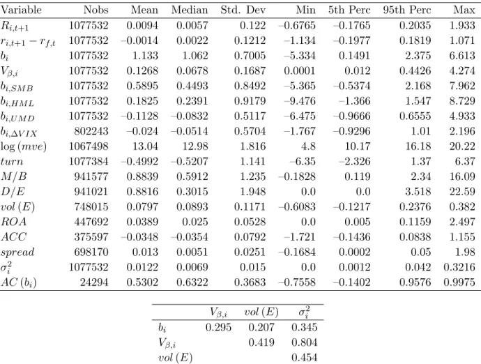
We document evidence that is consistent with our main prediction, using Fama-MacBeth regressions on the cross-section of CRSP stock returns. In the first stage, we estimate sixty month rolling window firm-specific regressions to estimate firm-specific factor loadings on the (log) excess market return, and use the standard error of the factor-loading estimate as a firm-specific proxy for factor-loading uncertainty. In the second-stage cross-sectional regressions, we show that uncertainty about market-factor loadings is negatively related to expected returns. We also find that this relation is statistically significant and is robust to including factor loadings on the SMB, HML, and UMD portfolios and aggregate volatility risk, and a number of firm characteristics (including size, market-to-book ratio, turnover, debt-to-equity ratio, volatility of earnings, return on assets, accruals, and bid-ask spreads). Moreover, the effect appears to be economically significant. In our sample of firms from January 1964 to December 2011, our estimates imply that a firm with the median level of uncertainty about the market-factor loading should have average annualized returns that are 400 to 525 basis points lower than an otherwise comparable firm with the same average factor loading but no uncertainty.
The next section discusses the marginal contribution of our paper in relation to the existing
5As Ang, Hodrick, Xing, and Zhang (2006) discuss, most models that incorporate market frictions or behav-ioral biases imply that idiosyncratic volatility should be positively related to expected returns. As such, they state that their “results on idiosyncratic volatility represent a substantive puzzle.”
literature. Section 2 presents the benchmark model, which we use to illustrate the intuition behind our main result. Section 3 presents the general model, which incorporates persistence in factor loadings and learning by investors, and characterizes the economic magnitudes of the effects we describe. Section 4 reports the results from our empirical analysis of the model’s main prediction and summarizes additional implications, and Section 5 concludes. All proofs are in Appendix A.
1.
Related Literature
Our paper relates most closely to P´astor and Veronesi (2003) and Xia (2001), but our results differ significantly from theirs. P´astor and Veronesi (2003) show that since a firm’s stock price is convex in its cash-flow growth, higher uncertainty about profitability leads to higher market-to-book ratios. Like P´astor and Veronesi (2003), we find that firm-specific uncertainty leads to higher valuations, and when investors learn about this source of firm-specific uncertainty, price-dividend ratios and idiosyncratic volatility exhibit time-series variation. However, P´astor and Veronesi (2003) and Johnson (2004) argue that for unlevered firms, learning about firm-specific profitability has no effect on expected returns.6 In contrast to these earlier papers, we
show that firm-specific uncertainty can have an effect on expected returns even in the absence of leverage. As we discuss further in Section 2, this is because the firm-specific uncertainty in our model is about the covariance between cash-flow growth and the pricing kernel, and, importantly, because this firm-specific uncertainty is resolved simultaneously with aggregate uncertainty.
As in Xia (2001), investors in our model learn about the predictability of expected returns, and this leads to stochastic variance of the factor loading. However, in contrast to Xia (2001), investors’ learning affects the pricing of returns in our model, and hence the stochastic condi-tional variance that results from learning leads to stochastic volatility in returns. While the effect of learning in generating stochastic return volatility has been explored at the aggregate level (e.g., David 1997; Veronesi 1999), to our knowledge, our model is the first to highlight a natural link between learning about factor loadings from past dividends / returns and stochastic volatility.
Our paper is also related to the large literature on parameter uncertainty and estimation risk. Kumar, Sorescu, Boehme, and Danielsen (2008) extend this literature by considering an economy in which investors are uncertain about the quality of information they can learn from. They endogenously derive a conditional CAPM in which the market risk premium, market volatility, and systematic risk of stocks depend on the information available to investors. Adrian and Franzoni (2009) extend the conditional CAPM by introducing unobservable long-run changes in factor loadings. They show that when investors learn about these long-long-run changes over time, the model generates low-frequency variation in betas that can help explain
6P´astor and Veronesi (2003) show that there is no effect of uncertainty about profitability on expected returns in the case of no dividends, and a small, local effect in the presence of dividends. Johnson (2004) shows that in levered firms, an increase in idiosyncratic volatility (which increases total volatility but keeps the risk premium constant) decreases the expected return on their levered equity.
the value and size premia in the cross-section of stock returns. Our analysis, which we view as complementary to these studies, takes the pricing kernel as given and focuses on the effect of firm-specific uncertainty about factor loadings. As a result, although firm-specific information has an effect on expected returns, it is not through an effect on the market risk premium (in contrast to Kumar et. al. 2008). Moreover, by explicitly modeling dividends in a standard asset pricing setup, we are able to derive implications of uncertainty and learning for not only expected returns but also other firm-specific attributes such as price-dividend ratios and return volatility.
2.
Benchmark Model
2.1
Model setup
In this section, we consider a simple benchmark model in which dividend growth is assumed to be independent and identically distributed over time. Although this assumption is made primarily for tractability, it also makes the effect of uncertainty about risk-factor loadings on expected returns transparent. In the next section, we generalize the model to allow for persistence in factor loadings and learning by investors.
The evolution of the pricing kernel is given by: Mt+1 =Mtexp
−rf −12Vm−mt+1 where mt+1∼ N (0, Vm), (1)
and the mt+1 are i.i.d., normally distributed variables with mean zero and variance Vm. The
aggregate source of risk, or risk factor, in the economy is therefore driven by the random variable mt+1. This implies that the unconditional (log) risk-free rate is given by rf, since
−logEhMt+1
Mt
i
=rf + 12Vm− 12Vm =rf. (2)
The existence of a pricing kernel relies only on the assumption that there is no arbitrage in the economy, which makes the current setup quite general. In particular, this representation can capture a variety of pricing models, including consumption-based models and factor-based models, such as the CAPM.7
7For instance, in an endowment economy in which aggregate consumption growth follows a log-normal process, i.e., ∆ct+1 ≡ log (Ct+1/Ct) ∼ N µ, σ2c
, and the representative investor has power utility with a coefficient of relative risk-aversionγ and discount factoreδ, the pricing kernel (or stochastic discount factor) is given by the marginal utility of the representative investor, Mt+1
Mt =e
δCt+1
Ct −γ
= exp{δ−γ∆ct+1}, and the risk-free rate is given by: Rf = exp{rf} ≡1/E
hM t+1 Mt i = exp −δ+γµ−12γ2σ2
c ,which, in turn, implies that
Mt+1=Mtexp −rf−12γ2σc2−γ(∆ct+1−µ) ≡Mtexp −rf−12Vm−mt+1 , wheremt+1=γ(∆ct+1−µ)∼N 0, γ2σ2c andVm=γ2σ2c.
At the beginning of each period, investors’ beliefs about firm i’s dividends (or cash flows), at date t+ 1 are given by:
Di,t+1 =Di,texp
¯
di+βi,t+1mt+1+di,t+1− 12 βi,t2 +1Vm+Vd,i , where di,t+1 ∼ N(0, Vd,i)
(3) and βi,t+1 is assumed to have an i.i.d. distribution given by
βi,t+1 ∼ N (bi, Vβ,i), (4)
and mt+1, di,t+1, and βi,t+1 are independent. The specification in equation (3) implies that dividend growth consists of a constant component (i.e., ¯di), a systematic component (i.e.,
βi,t+1mt+1), and an idiosyncratic component (i.e.,di,t+1). The systematic component of dividend growth depends on the firm’s stochastic factor loading, βi,t+1.8 Unlike standard models, we relax the assumption that investors know (with certainty) the future factor loading that drives dividend growth at time t+ 1. We first assume that factor loadings are i.i.d. over time to highlight the intuition for our main result, but we relax this assumption in the next section.
Our specification also ensures that (log) expected dividend growth is given by ¯di. In the
standard case, when there is no uncertainty about βi,t+1 = bi, one can adjust the dividend
growth process by a convexity adjustment term 1 2b
2
iVm + 12Vd,i to ensure that (log) expected
dividend growth is given by ¯di, i.e.,
Di,t+1 =Di,texp
¯ di+bimt+1+di,t+1− 12 b2iVm+Vd,i ⇒ E hD i,t+1 Di,t i = exp¯ di (5)
In our setup, the convexity adjustment naturally generalizes to 12β2
i,t+1Vm+12Vd,i, which implies
that the log expected dividend growth is given by ¯di, since
EhDi,t+1 Di,t i =E E exp¯
di+βi,t+1mt+1+di,t+1− 12 βi,t2 +1Vm+Vd,i βi,t+1
= exp¯
di .
(6) This convexity adjustment ensures that the effect of uncertainty about βi,t+1 that we derive is not simply a consequence of the difference between log expected returns and expected log returns.9
2.2
The pricing equation and expected returns
By the definition of the pricing kernel, the price of firm i’s stream of dividends is given by: Pi,t =Et " ∞ X s=1 Mt+s Mt Di,t+s # , (7)
8This is an example of what is known as a random coefficients model (e.g., Cooley and Prescott 1976). Ang and Chen (2007) use a similar setup to model the uncertainty faced by an econometrician when estimating time-varying betas, and use this to argue that there is little evidence of a value premium in the long run.
9One can alternatively define the convexity adjustment as logEhDi,t+1
Di,t i −EhlogDi,t+1 Di,t i . As we show in Appendix B, while this alternative specification implies a similar (but larger) effect of uncertainty aboutβi,t+1 on the expected return, it leads to less-transparent and less-intuitive expressions for expected returns.
and the unconditional expected return on the firm’s dividend stream is then given by: E[Ri,t+1] =E h Pi,t+1+Di,t+1 Pi,t i . (8)
Under an appropriate transversality condition, we have our benchmark result.
Proposition 1. Suppose the sequence of prices Pt satisfies the following transversality
condi-tion: lim T→∞Et h Mt+T Mt Pt+T i = 0. (9)
Then, given that factor loadings are i.i.d., we have the following results:
(a) firm i’s price-dividend ratio is constant, and given by P Di,t ≡Pi,t/Di,t = 1−pipi, where
pi =E h Mt+1 Mt Di,t+1 Di,t i = exp¯ di −rf −biVm+ 12Vβ,iVm2 , (10)
(b) firm i’s return process is of the form:
Ri,t+1 = exp
µi+βi,t+1mt+1+di,t+1− 12 βi,t2 +1Vm+Vd,i , (11)
(c) firm i’s expected return is given by: E[Ri,t+1] = exp{µi}= exp
rf +biVm− 12Vβ,iVm2 . (12)
The result implies that conditional on the (mean) level of the factor loading (i.e.,bi), higher
uncertainty about the factor loading (i.e., Vβ,i) decreases firm i’s expected return. This result
follows from the effect of uncertainty about βi,t+1 on the covariance between dividend growth and the pricing kernel. To understand this effect, we derive the expression for the covariance explicitly: covMt+1 Mt , Di,t+1 Di,t =EhcovMt+1 Mt , Di,t+1 Di,t βi,t+1 i + covEhMt+1 Mt βi,t+1 i ,EhDi,t+1 Di,t βi,t+1 i =EhcovMt+1 Mt , Di,t+1 Di,t βi,t+1 i (13) =E exp¯ di−rf (exp{−βi,t+1Vm} −1) (14) = exp¯ di−rf exp −biVm+ 12Vm2Vβ,i −1 . (15)
Since the expected value of the pricing kernel and dividend growth conditional on a realization ofβi,t+1 are uncorrelated, the unconditional covariance between the pricing kernel and dividend growth is just the expectation of the covariance conditional on a realization of βi,t+1 (i.e., it is given by (13)). Moreover, since conditional on a specific realization of βi,t+1, MMt+1t and DDi,ti,t+1 are lognormal random variables, the covariance between them is a convex function of βi,t+1 (see the expression in equation (14)). As a result, the unconditional covariance between the pricing kernel and dividend growth is increasing in uncertainty about βi,t+1 through a Jensen’s inequality effect.
The convexity of the conditional covariance (given by equation (14)) inβi,t+1follows from our assumption that both the pricing kernel and dividend growth are log-linear (convex) functions of the common shock mt+1. This is a common assumption in much of the asset pricing literature, which relies on the exponential-affine structure of the setup. Intuitively, the log-linearity implies that the pricing kernel Mt+1
Mt is steeper in bad states of the world (i.e., low mt+1, or high
Mt+1
Mt )
than in good states of the world (i.e., highmt+1, or low MMt+1t ). In a representative agent model, this can be interpreted as the convexity of the representative agent’s marginal utility—the agent’s marginal utility is steeper in bad states of the world (i.e., low aggregate consumption) than in good states of the world.
The convexity of the pricing kernel implies that the present value of a dividend Di,t+1 in the next period, given by Mt+1
Mt Di,t+1, is convex in the factor loading βi,t+1. As a result, a
mean-preserving spread inβi,t+1 increases the present value of the dividend. Intuitively, in bad states of the world, the effect of a unit decrease in βi,t+1 (i.e., a decrease in systematic risk) leads to a bigger increase in the present value of the dividend than the decrease in its present value from a unit increase in βi,t+1. In good states of the world, the opposite is true i.e., the effect of an increase in βi,t+1 is bigger. As a result, a mean-preserving spread inβi,t+1 increases the present value of the dividend in both good and bad states of the world. Figure1illustrates these effects for a specific set of parameters. The bottom panel plots the present value of the dividend across states of the world given a mean-preserving spread in βi,t+1 (of ±0.1 around one). For bad states of the world (i.e., mt+1 ≤ 0), the effect of a decrease in βi,t+1 on the present value is larger, while for good states of the world, the effect of an increase in βi,t+1 is larger. Consequently, the effect of a mean-preserving spread is to increase the present value of the dividend (i.e., the average of the dashed and dotted lines lies above the solid line), or, equivalently, decrease the expected return.
As we show in the proof of Proposition1, since the pricing kernel and cash-flow growth are conditionally independent over time, the price-dividend ratio (denoted by P Di,t) is constant.
Moreover, the effect of uncertainty on the present value of the dividend is also reflected in the expression for the price-dividend ratio. In particular, a firm’s price-dividend ratio P Di,t
is increasing in the price-dividend ratio of a dividend strip, pi, which itself is increasing in
uncertainty aboutβi,t+1(see equation (10)). This effect of uncertainty on valuations is analogous to the effect of uncertainty about profitability on market-to-book ratios in P´astor and Veronesi (2003).
Since the price-dividend ratio is constant, the Euler equation EhMt+1
Mt Ri,t+1
i
= 1 implies that the expected excess return on securityidecreases with the covariance between its dividend growth and the pricing kernel, which, in turn, implies that it is decreasing in the uncertainty about its factor loading, since
E[Ri,t+1]−Rf =−Rfcov
Mt+1
Mt , Ri,t+1
=−Rf1+P DP Di,ti,t cov
Mt+1 Mt , Di,t+1 Di,t (16) =−Rfp1icov Mt+1 Mt , Di,t+1 Di,t =Rf expbiVm− 12Vβ,iVm2 −1 . (17) As we show in the next section, if the factor loading is persistent, the price-dividend ratio varies over time, and this amplifies the effect of factor-loading uncertainty on expected returns.
However, by initially shutting down this additional effect, we are able to characterize the effect of factor-loading uncertainty on expected returns more transparently.
Expression (11) for returns in Proposition1explicitly accounts for the appropriate convexity adjustments (through the 1
2 β 2
i,t+1Vm+Vd,i term), and as such, our main result is not simply
an artifact of the difference between log expected returns and expected log returns.10 Finally,
since there is only one source of aggregate uncertainty, the risk-factor loading that drives firm i’s cash-flow growth also drives the covariance of the firm’s return with the pricing kernel. Accordingly, if there is a tradable factor-mimicking portfolio, then our model implies a log-linear, uncertainty-adjusted CAPM that is described in the following corollary.
Corollary 1. Suppose RM,t+1 is the return on the factor-mimicking portfolio—i.e.,
RM,t+1 = exp
µM +mt+1− 12Vm , (18)
where µM = log (E(RM,t+1)) denotes the log expected return. Then the log expected return
µi = log (E(Ri,t+1))on firm i’s stock with cash-flow loadingβi,t+1 ∼N(bi, Vβ,i) is characterized
by the following expression:
µi−rf =bi(µM −rf)− 12Vβ,iVm2. (19)
Moreover, conditional on βi,t+1, the covariance between ri,t+1 = log (Ri,t+1) and rM,t+1 = log (RM,t+1) is given by βi,t+1Vm.
The above result immediately follows from the definition of the factor-mimicking portfolio RM,t+1 and Proposition 1. The corollary highlights that, in our model, risk-factor loadings in cash-flow growth are identical to risk-factor loadings in log returns. The corollary also highlights that while firm-specific uncertainty about factor loadings (i.e., Vβ,i) affects expected returns,
uncertainty about the idiosyncratic component of dividend growth (i.e.,Vd,i) does not. Finally,
in the special case of our model where investors face no uncertainty about risk-factor loadings (i.e., Vβ,i = 0), we recover the standard log-linear CAPM relation, which is given by
µi−rf =bi(µM −rf). (20)
2.3
Discussion
Although our model is very similar to those in P´astor and Veronesi (2003) and Johnson (2004), in contrast to those studies, we find that firm-specific parameter uncertainty has an effect on expected returns even in the absence of leverage.11 As noted in these earlier papers, whether
parameter uncertainty affects expected returns depends not only on what parameters investors are uncertain about, but also when the parameter uncertainty is resolved. In our model,
10Specifically, the object of interest is the log expected return,µ
i, which is characterized in equation (12).
11As mentioned earlier, P´astor and Veronesi (2003) show that there is no effect of uncertainty about prof-itability on expected returns in the case of no dividends, and a small, local effect in the presence of dividends. However, the mechanism through which firm-specific uncertainty affects expected returns in our model is dif-ferent and, as we discuss in the next section, is potentially substantial in magnitude.
uncertainty about βi,t+1 affects expected returns because (i) βi,t+1 affects prices and returns nonlinearly,and (ii) the risk generated by the parameter uncertainty isresolved simultaneously
with aggregate uncertainty (i.e., uncertainty aboutβi,t+1andmt+1are resolved simultaneously). While the log-normal framework we use is tractable and helps us relate our results to the literature, these observations suggest that uncertainty about factor loadings should have an effect on expected returns in other settings if conditions (i) and (ii) are satisfied.12 In a related
point, note that, in our model, investors face uncertainty about the covariance between cash-flow growth and the pricing kernel, and the nonlinearity this introduces is important for our results. As such, the effect of uncertainty on expected returns would be different in a model where investors face uncertainty about thelevel of cash flows or prices, instead of the risk-factor loadings.
It is also important to note that investors do not “eventually learn” the factor loading of a firm’s dividends in our model. Given the distribution of βi,t+1 in (4), investors always face residual uncertainty about the future factor loadings of a firm’s dividends. Moreover, since factor loadings are stochastic, regressingpast dividend growth on past realizations of the aggregate risk factor only provides investors with an estimate of past factor loadings, but does not perfectly reveal future factor loadings, which are relevant for setting current prices. As we show in the next section, this is true even when factor loadings are persistent.
3.
Learning About Persistent Factor Loadings
In this section, we generalize the model by allowing for persistence in firm’s risk-factor load-ings. We show that the effect of factor-loading uncertainty on expected returns is generally amplified when βi,t are persistent. We also show that since price-dividend ratios depend on
investors’ conditional beliefs, learning about factor loadings generates time-series variation in price-dividend ratios and, as a result, is an additional source of variation in returns.
We maintain most of the assumptions of the benchmark model. In particular, investors’ beliefs about the pricing kernel and firm i’s dividend process are given by (1) and (3), respec-tively. However, we generalize the process for the risk-factor loading to allow for persistence by assuming that βi,t+1 evolves according to the following process:
βi,t+1 = (1−ai)bi+aiβi,t+φiyt+νi,t+1, whereνi,t+1∼N(0, Vβ,i), yt ∼N(0, Vy) (21)
and νi,t+1 and yt are independent of each other and independent ofmt+1 anddi,t+1. We assume that the persistence,ai, the unconditional mean,bi, the fundamental variance of factor loadings,
Vβ,i, the conditioning variable yt, and the corresponding weight, φi, are known to all investors
at date t, but that the realization ofβi,t is not. Without loss of generality, we assume that the
conditioning variableyt is mean zero, so that the unconditional mean ofβi,t+1 isbi. We restrict
attention to the simplest specification that allows for persistence in factor loadings to maintain tractability and to highlight the effect of uncertainty and learning in a transparent manner.
12For instance, our example in the introduction illustrates the effect of factor-loading uncertainty on expected returns in a setting that does not assume log-normality.
The specification in equation (21) is a special case of Adrian and Franzoni (2009) applied to our log-linear setting, and, as discussed in their paper, nests a number of conditional CAPM models as special cases (including Jagannathan and Wang 1996; Lettau and Ludvigson 2001; Jostova and Philipov 2005; Ang and Chen 2007).
It is important to note that we maintain the assumption that Vm is constant over time,
which implies that the aggregate risk premium (or, market price of risk) for the economy remains constant. While we believe that time-series variation in the aggregate risk premium is empirically and theoretically important, we make this assumption to highlight the effects of learning about factor loadings in our setting. In particular, any time-series variation in expected returns and price-dividend ratios will not be driven by time-series variation in the market price of risk, but by the learning process of investors.
In the following subsections, we consider different models of learning. Subsection 3.1 de-scribes the general version of the model in which investors learn about the current realization of βi,t using exogenous signals. In Subsection 3.2, we consider two special cases to refine the
intuition from the general model, and to gauge the economic magnitude of the effects we char-acterize. In Subsection 3.3, we present an extension of the general model in which investors condition on realized dividends and returns to update their beliefs about βi,t. In this case, we
show that learning can induce stochastic volatility in the return process, even if all fundamental shocks are assumed to be homoscedastic.
3.1
Learning from signals
Although we explicitly model how investors can learn about factor loadings from realized div-idends and returns in a later extension, we begin with a stylized information structure that provides a useful benchmark. We assume that investors do not observe the factor loadings themselves, but that they instead observe a signal Yi,t+1 at datet+ 1, given by
Yi,t+1 =βi,t+1+εi,t+1, whereεi,t+1 ∼N(0, Vε,i,t), (22)
and εi,t+1 is uncorrelated with mt+1, yt+1, βi,t+1, and di,t+1. Although we allow εi,t+1 to have time-varying volatility, we assume that conditional on datet information, the volatility ofεi,t+1 is known to investors. This assumption allows us to parsimoniously model the possibility of time-series variation in information quality, without introducing too much additional notation or complexity. One can interpret the information structure in equation (22) as a reduced-form representation of investors learning about factor loadings from a variety of information sources that we do not model explicitly, including fundamental analysis, earnings announcements and guidance, and firm-level disclosures (e.g., see Beaver, Kettler, and Scholes 1970; Bowman 1979). The stylized nature of (22) allows us to characterize the first-order effects of learning in a tractable manner, and we leave more nuanced modeling of richer information structures for future work.
Denote investors’ distribution ofβi,t+1 conditional on date t information by
Given the evolution of factor loadings and the information structure above, an immediate application of the Kalman filter gives us the following result.
Lemma 1. The expectation of the risk-factor loading at date t+ 2, conditional on the infor-mation available to investors at date t+ 1, is given by:
bi,t+1 ≡Et+1[βi,t+2] = (1−ai)bi+ai(bi,t+λi,t(Yi,t+1−bi,t)) +φiyt+1 (24) = (1−ai)bi+ai(bi,t+λi,t(βi,t+1+εi,t+1−bi,t)) +φiyt+1 (25) where λi,t = Σi,tΣ+i,tVε,i,t. The variance of the risk-factor loading at date t+ 2, conditional on date
t+ 1 information, is given by:
Σi,t+1 ≡vart+1(βi,t+2) =Vβ,i+a2iΣi,t(1−λi,t). (26)
Moreover, if the quality of information available to investors is constant (i.e., Vε,i,t =Vε,i), then
the steady-state conditional variance is given by:
Σi = 1−a21 i(1−λi)Vβ,i= 1 2 Vβ,i−Vε,i 1−a2i + q
4Vβ,iVε,i+ (Vβ,i−Vε,i(1−a2i))
2
, (27)
where λi = Σi+ΣViε,i.
The Kalman gain parameter, λi,t, is a convenient measure of the quality of information
available to investors at date t, since it is decreasing in the noise of the signal, Vε,i,t, and
is bounded between zero and one. The gain λi,t is zero when the noise in the signal Yi,t is
infinite (i.e., Vε,i,t → ∞) and investors learn nothing about the factor loading from their signal.
Conversely, the gain is one if the noise in the signal is zero, and investors perfectly learn the current realization of βi,t from their signal. As expected, the conditional variance of factor
loadings at date t is decreasing in the quality of information available to investors at date t (i.e., λi,t).
If the quality of information available to investors is constant (i.e., Vε,i,t = Vε,i), then we
can characterize the steady-state value of the conditional variance in closed form (see equation (27)). Straightforward calculations also imply the following intuitive results:
lim λi→1 Σi =Vβ,i, lim λi→0 Σi = 1−1a2 iVβ,i, ∂ ∂Vβ,iΣi >0, and ∂ ∂Vε,iΣi >0. (28)
If the quality of information available to investors is perfect (i.e., λi = 1, or Vε,i = 0), then
investors observe the realization of the current factor loading perfectly, and the conditional variance of the next period’s factor loading is given by Vβ,i. As such, even if investors perfectly
observe current factor loadings, they still face uncertainty about future loadings that are relevant for pricing returns. At the other extreme, if the signal Yi,t is infinitely noisy (i.e., Vε,i → ∞,
or λi → 0), then investors have no information about the current factor loading, and the
conditional variance of the next period’s factor loading is given by the unconditional variance 1
1−a2
iVβ,i. This quantity characterizes the upper bound on the uncertainty that investors face
Given the evolution of beliefs described in Lemma1, we can calculate firmi’s price-dividend ratio and returns by log-linearizing the price-dividend ratio around its long-run mean (e.g., Campbell and Shiller 1988). Under the appropriate transversality condition, we have our main result.
Proposition 2. Suppose the sequence of prices Pt satisfies the following transversality
condi-tion: lim T→∞Et h Mt+T Mt Pt+T i = 0. (29)
Then, given that factor loadings evolve according to (21), and investors’ beliefs evolve according to the results of Lemma 1, a log-linearization of the price-dividend ratio around its long-run mean implies the following:
(a) firm i’s log price-dividend ratio is given by:
pdi,t = log (P Di,t) =Ai,t −1−1ρiaibi,tVm, (30)
(b) firm i’s return process is of the form:
Ri,t+1 = exp
αi,t+βi,t+1mt+1+di,t+1− 12 βi,t2 +1Vm+Vd,i
+γibi,t+1 , (31) (c) firm i’s expected return, conditional on date t information, is given by:
Et[Ri,t+1] = exp n rf +bi,tVm− 12 1 + 2λi,t1−aiaρiiρi Σi,tVm2 o , (32)
where Ai,t, αi,t, and γi are known to investors at date t, and defined in Appendix A, and
ρi ≡
exp{pd¯}
1+exp{pd¯} ∈(0,1), where pd¯ is the long-run mean of pdi,t.
The above proposition presents our main results, and generalizes the benchmark results of Proposition 1. As before, the price-dividend ratio is decreasing in the conditional mean bi,t,
and increasing in the conditional variance of the factor loading (i.e., Σi,t), as can be seen from
expression (A10) for Ai,t in Appendix A. As in the i.i.d. case, since the systematic shocks to
returns are driven byβi,t+1mt+1, the covariance between firmi’s return and the factor-mimicking portfolio is still driven by the factor loading—i.e., the covariance between ri,t+1 = log (Ri,t+1) and rM,t+1 = log (RM,t+1) (as defined by (18)) is given by βi,t+1Vm. Finally, as in Proposition
1, firm i’s expected return is decreasing in investors’ (conditional) uncertainty about its factor loadings (i.e., Σi,t), even after controlling for the conditional mean level of its factor loading
(i.e., bi,t).
However, allowing for persistence in firms’ factor loadings generates a number of additional effects that are not present in the benchmark case of Proposition 1. First, a firm’s price-dividend ratio is no longer constant, but instead depends on investors’ conditional beliefs about its factor loadings. This implies that a firm’s price-dividend ratio varies over time, even when all fundamental shocks have constant variance by assumption, and in particular, the aggregate risk premium (i.e., Vm) is constant. Moreover, this time-series variation in price-dividend ratios
leads to an additional source of variation in returns. In particular, a firm’s returns depend not only on shocks to its dividend growth (as captured byβi,t+1mt+1+di,t+1), but also on variation in investors’ beliefs about its factor loading (as captured by bi,t+1).
The effect of investors’ uncertainty about factor loadings (i.e., Vβ,i) on expected returns is
increasing in the persistence of factor loadings (i.e., ai). This amplification effect manifests
through two complementary channels. To illustrate the intuition for this effect, consider the following expression for firm i’s expected excess return:13
Et[Ri,t+1]−Rf =−Rfcovt Mt+1 Mt , Ri,t+1 =−Rfcovt Mt+1 Mt , 1+P Di,t+1 P Di,t Di,t+1 Di,t (33) =−RfEt h covt Mt+1 Mt , Di,t+1 Di,t βi,t+1 1+P D i,t+1 P Di,t i (34) =−RfEt h exp¯
di−rf (exp{−βi,t+1Vm} −1)1+P DP Di,ti,t+1
i
(35) The first channel through which persistence affects expected returns is through its effect on the conditional covariance between the pricing kernel and dividend growth. As in the i.i.d. case, the covariance between the pricing kernel and dividend growth, conditional on a realization of βi,t+1, is a convex function of βi,t+1 (see equation (35)). Moreover, as Lemma 1 implies, the conditional variance of factor loadings (i.e., Σi,t) ranges from a lower bound ofVβ,ito an upper
bound of 1 1−a2
iVβ,i, and is increasing in Vβ,i. Hence, even if price-dividend ratios were constant
(as in the i.i.d. case), the effect of the same level of fundamental uncertainty (i.e., Vβ,i) on the
conditional covariance is at least as large as in the i.i.d. case, but is likely to be larger, when factor loadings are persistent (i.e., ai >0).
Second, a larger variance of shocks to factor loadings (i.e., a higherVβ,i) leads to a higher
volatility of conditional expectations (i.e., higher vart(bi,t+1)), which translates into a larger multiplicative effect on the expected excess return through the 1+P Di,t+1
P Di,t term, since P Di,t+1
is convex in the conditional expectation bi,t+1. Intuitively, since factor loadings are persistent, price-dividend ratios are correlated over time. This implies that, when investors learn about the current factor loading, βi,t, they update their beliefs about the covariance between dividends
and the pricing kernel not only for the next period, but for all future periods. The effect of this amplification on the current price-dividend ratio is captured by the factor 1−1ρiai, which scales bi,tVm in equation (30). Similarly, the amplification effect on expected returns is captured by
the 2λi,t1−aiaρiiρi term in equation (32).
Proposition2 also highlights that in a dynamic setting, an increase in fundamental uncer-tainty about factor loadings (i.e., higherVβ,i) and a decrease in information quality about factor
loadings (i.e., lower λi, or higher Vε,i) can have different effects. In static settings, as intuition
suggests, an increase inVβ,ihas a similar effect as a decrease inλi, since both lead to an increase
in conditional uncertainty (i.e., Σi). However, in a dynamic setting, information quality affects
13Mathematically, note that since both the price-dividend ratio (i.e., P D
i,t+1) and the covariance be-tween the pricing kernel and dividend growth, conditional on βi,t+1 (i.e., covt
M t+1 Mt , Di,t+1 Di,t βi,t+1 ) are log-convex in βi,t+1, so is their product (see equation (34)). This, in turn, implies that the product covt M t+1 Mt , Di,t+1 Di,t βi,t+1 1+P D i,t+1
P Di,t is convex in βi,t+1, and so the expected excess return is decreasing in
future uncertainty in two offsetting ways. To see these channels explicitly in our model, note that Proposition2implies that the effect of uncertainty on expected returns in the steady state is given by the following term:
−1 2 1 + 2λi1−aiaρiiρi ΣiVm2, where Σi = 1−a21 i(1−λi)Vβ,i. (36)
This expression shows that information quality has two offsetting effects on expected returns when factor loadings are persistent. First, as in a static model, higher information quality (i.e., higher λi) decreases the conditional uncertainty about future factor loadings (i.e., lowers
Σi). However, higher information quality also increases the sensitivity of expected returns to
uncertainty about factor loadings through the 2λi1−aiaρiiρi term. This is because, in a dynamic
setting, higher information quality also implies that investors put more weight on their signals when updating their beliefs, which, in turn, implies that conditional expectations are more volatile in the future (i.e., higher variance of bi,t). The overall effect of information quality
(i.e., λi) on expected returns depends on both of these effects. In particular, by differentiating
expression (36) with respect to λi, one can show that the relation between expected returns
and information quality after controlling for the level of factor-loading uncertainty (i.e.,Vβ,i) is
positive when factor-loading persistence is high enough—i.e., when ai−2ρi+a2iρi >0, or equivalently, ai > 21ρi q 1 + 8ρ2 i −1 , (37)
but negative when factor-loading persistence is low (i.e., when ai < 21ρi
p 1 + 8ρ2 i −1 ).14
The subtle difference between the notions of uncertainty and information quality in a dy-namic setting may have important empirical implications. For instance, our model predicts that the cross-sectional effect of an increase in fundamental uncertainty about factor loadings (i.e., Vβ,i) is to decrease expected returns. However, after controlling for the level of
fundamen-tal uncertainty (i.e., Vβ,i), our model predicts that expected returns decrease with information
quality when factor-loading persistence (i.e., ai) is low, but increase with information quality
when factor-loading persistence is high.
Similarly, one must be careful when distinguishing between the effects of uncertainty and information quality on return volatility, as the next result suggests.
Corollary 2. Conditional on date t information, and adjusting for convexity effects, the id-iosyncratic volatility of log returns ri,t+1 = log (Ri,t+1), is given by σi,t, where
σi,t2 ≡vart ri,t+1− βi,t+1mi,t+1− 12βi,t2+1Vm
=Vdi+ ρi 1−ρiaiVm 2 a2 iΣ2i,t Σi,t+Vε,i,t +φ 2 iVy . (38)
14This mechanism through which higher information quality can lead to higher uncertainty can be found in other dynamic settings. For instance, Banerjee (2011) highlights a similar effect in a dynamic version of Hellwig (1980)’s rational expectations model. In the model, investors receive private signals about next period’s dividends, but also condition on prices to update their beliefs. When the quality of investors’ information improves, their posterior uncertainty about next period’s dividends decreases, but the total risk they face may increase. This is because, as a result of more precise signals, prices are more sensitive to investors’ signals and are therefore more volatile. Since investors care about future dividends and future prices, the total risk they face may actually increase as information quality improves.
Note that since factor loadings are stochastic in our model, the systematic component of re-turn volatility is stochastic by construction. Since we want to identify the effect of factor-loading uncertainty and learning on volatility that is not mechanically driven by our assumptions, we focus on the volatility of the idiosyncratic component of returns.
The result shows that idiosyncratic volatility is driven by the volatility of idiosyncratic shocks to dividend growth (i.e., Vd,i) and the volatility of investors’ future conditional
expec-tations of factor loadings (i.e., vart(bi,t+1)). As a result, idiosyncratic volatility is increasing in investors’ conditional variance of factor loadings (i.e., Σi,t), the variance of shocks to
divi-dend growth (i.e.,Vd,i), and the variance of conditioning variables that investors use to forecast
factor loadings (i.e., Vy). Idiosyncratic volatility is also increasing in the persistence of factor
loadings (i.e., ai) and the volatility of the aggregate risk factor (i.e, Vm), since an increase in
either variable implies that bi,t+1 has a bigger impact on current returns. Finally, the result implies that if the quality of information available to investors is time-varying (i.e., if Vε,i,t
varies over time), then idiosyncratic volatility also exhibits time variation. Moreover, all else equal, the conditional idiosyncratic volatility at date t increases with information quality λi,t
(i.e., decreases with Vε,i,t), after controlling for uncertainty (i.e., Σi,t). As discussed above, this
is because lower information quality (i.e., higher Vε,i,t) implies a noisier signal Yi,t+1, which, in turn, implies a lower sensitivity of bi,t+1 to Yi,t+1, and therefore lower variability of bi,t+1 (i.e., lower vart(bi,t+1)).
Note that Proposition2and Corollary 2together imply that controlling for the variation of factor-loading uncertainty, variation in information quality (i.e., λi,t) leads to a positive relation
between expected returns and idiosyncratic volatility when factor-loading persistence is high enough (i.e., ai > 21ρi p 1 + 8ρ2 i −1
), but a negative relation when factor-loading persistence is low. As such, we expect to find the relation between expected returns and idiosyncratic volatility, after controlling for factor-loading uncertainty, to be more positive for firms with more persistent factor loadings. In Section 4, we test this prediction on the cross-section of stock returns and find evidence consistent with the prediction (see Table 4).
3.2
Special cases
In this subsection, we consider two extreme special cases of the general model to develop a better understanding of the effects of uncertainty and learning on return dynamics, and to gauge the economic magnitude of these effects. In the first case, we assume that investors receive no signals about the current realization of the factor loading (i.e., βi,t), and so they
price securities based on the unconditional distribution of βi,t. In the second case, we assume
that investors observe βi,t perfectly at date t. Together, these two cases characterize the range
of possible effects that uncertainty and learning can have on prices and returns. Without much loss of generality, we simplify the exposition of this analysis by setting φi to zero.
When investors receive no signals about factor loadings at datet(or equivalently, if the noise in signals is infinite—i.e.,Vε,i,t→ ∞), then investors calculate prices and expected returns based
on the unconditional distribution of βi,t+1, which is given by βi,t+1 ∼N bi, 1−1a2 iVβ,i . (39)
Since investors have no information about either the current or future values of βi,t, investor
uncertainty about factor loadings is highest in this case. Moreover, price-dividend ratios and expected returns are constant over time, and are characterized by the following corollary to Proposition 1.
Corollary 3. Suppose the sequence of prices Pt satisfies the following transversality condition:
lim T→∞Et h Mt+T Mt Pt+T i = 0. (40)
Then, given that factor loadings evolve according to (21), and investors’ beliefs are given by
(39), we have the following:
(a) firm i’s price-dividend ratio is constant, and given by P Di,t ≡Pi,t/Di,t = 1−pipi, where
pi = exp ¯ di−rf −biVm+2(1−1a2 i) Vβ,iVm2 , (41)
(b) firm i’s return process is of the form
Ri,t+1 = exp
µi+βi,t+1mt+1+di,t+1− 12 βi,t2 +1Vm+Vd,i , (42)
(c) firm i’s expected return is given by Et[Ri,t+1] = exp{µi}= exp
rf +biVm− 2(1−1a2 i) Vβ,iVm2 , and (43)
(d) the idiosyncratic volatility of log returns, ri,t+1 = log (Ri,t+1) is given by σi,t, where
σi,t2 ≡vart ri,t+1− βi,t+1mi,t+1− 12βi,t2+1Vm
=Vd,i. (44)
When investors do not receive any information about firms’ factor loadings, their conditional and unconditional beliefs coincide, and as a result, the expressions for prices and expected re-turns look similar to those in the benchmark model in Section 2. However, the effect of uncer-tainty is magnified by a factor of 1/(1−a2
i) relative to the i.i.d. case, since the unconditional
variance of βi,t+1 is given by (1−1a2
i)
Vβ,i. Finally, since there is no time-series variation in the
conditional expectation of future factor loadings, the idiosyncratic volatility of log returns is simply given by the volatility of idiosyncratic shocks to dividend growth (i.e., Vd,i).
At the other extreme, the investor uncertainty about factor loadings is lowest when investors can perfectly observe the realization of βi,t at date t (or equivalently, if the noise in signals is
zero—i.e., Vε,i,t = 0) . In this case, the conditional distribution of βi,t+1, given investors’ information at date t, is given by
βi,t+1|It ∼N((1−ai)bi +aiβi,t, Vβ,i), (45)
Corollary 4. Suppose the sequence of prices Pt satisfies the following transversality condition: lim T→∞Et h Mt+T Mt Pt+T i = 0. (46)
Then, given that factor loadings evolve according to (21), and investors’ beliefs are given by (45), a log-linearization of the price-dividend ratio around its long-run mean implies the following:
(a) firm i’s price-dividend ratio is given by
pdi,t = log (P Di,t) = Ai,t− 1−1ρiai((1−ai)bi+aiβi,t)Vm (47)
(b) firm i’s return process is of the form
Ri,t+1 = exp
αi,t+βi,t+1mt+1+di,t+1− 12 βi,t2 +1Vm+Vd,i
+γibi,t+1 , (48) (c) firm i’s expected return, conditional on date t information, is given by
Et[Ri,t+1] = exp n rf + ((1−ai)bi+aiβi,t)Vm− 12 1 + 2 aiρi 1−aiρi Vβ,iVm2 o , and (49)
(d) the idiosyncratic volatility of log returns, ri,t+1 = log (Ri,t+1) is given by σi,t, where
σi,t2 ≡vart ri,t+1− βi,t+1mi,t+1−12βi,t2 +1Vm
=Vd,i + ρiai 1−ρiaiVm 2 Vβ,i, (50)
where Ai,t, αi,t, and γi are known to investors at date t, and defined as in Proposition 2 (with
bi,t = (1−ai)bi+aiβi,t and Σi,t = Vβ,i), and ρi ≡
exp{pd¯}
1+exp{pd¯} ∈ (0,1), where pd¯ is the long-run
mean of pdi,t.
Although investors observe the current realization of factor loadings perfectly, they still face uncertainty about future realizations of βi,t. As in the general case in Proposition 2, the
price-dividend ratio is log-linear in the conditional expectation of next period’s factor loading, which is given by ((1−ai)bi+aiβi,t) in this case. As before, the effect of uncertainty on
expected returns is increasing in Vβ,i and ai, since persistence in factor loadings implies that
uncertainty about next period’s factor loading leads to uncertainty about factor loadings in all future periods. Finally, as in the general case with imperfect learning, idiosyncratic volatility is driven by the volatility of idiosyncratic shocks to dividend growth (i.e., Vd,i) and the volatility
in the conditional expectations of future factor loadings, which in this case is given by a2
iVβ,i.
The two extreme cases characterized by Corollaries 3 and 4 imply that introducing persis-tence in factor loadings increases the effect of uncertainty on expected returns relative to the i.i.d. case from Section 2. However, as discussed in the previous subsection, the effect on ex-pected returns is not monotonic in the information quality of investors’ signal Yi,t. Specifically,
whether the effect of uncertainty is larger in the full-information case of Corollary 4 or the no-information case of Corollary 3 depends on the persistence in factor loadings, ai, and the
no-information case relative to the full-information case if and only if ρi < 2−aia2
i. The
expres-sions in Corollaries 3 and 4also highlight the result that, all else equal, idiosyncratic volatility decreases with the variance of the noise in the signals (i.e., Vε,i,t), since noisier signals about
factor loadings imply lower variability in conditional expectations about future factor loadings (i.e., vart(bi,t+1)).
Corollaries3 and 4also allow us to characterize the economic magnitude of these effects in a tractable manner. We present a numerical example in Figure 2. We plot expected returns as a function of Vβ,i for the i.i.d. case presented in Section 2, the no-information benchmark
presented in Corollary 3, and the full-information benchmark presented in Corollary 4. We set the risk-free rate to 2%, the variance of the pricing kernel Vm to 0.2, the unconditional
mean factor loading (i.e., bi) to 1, and the long-run mean price-dividend ratioP Di,t to 4, which
implies ρi = 0.80. The assumed value of Vm is consistent with a Sharpe ratio on the aggregate
stock market of at least 0.5.15 Although there is significant cross-sectional variation in firms’
price-dividend ratios, our estimate of the long-run mean P Di,t is chosen to be conservative
and to highlight the non-monotonic dependence of expected returns on information quality as described above.
The plots in Figure2suggest that the effect of uncertainty about factor loadings on expected returns can be economically significant, especially when factor loadings are persistent. In the i.i.d. benchmark model of Section 2, the effect is relatively small—a unit increase in the variance ofβi,t(i.e.,Vβ,i= 1) leads to a decrease in annualized expected returns of about 200 basis points.
However, once we allow for persistence, this effect is amplified considerably. For instance, with a persistence ofai = 0.85, a unit increase inVβ,icorresponds to a decrease in annualized expected
returns of between 520 and 850 basis points (for the no-information and full-information cases, respectively). And increasing the persistence to ai = 0.95 implies that a unit increase in Vβ,i
leads to a decrease of between 12 and 19 percent in annualized expected returns. The choice of mean P Di,t is conservative in that we expect the price-dividend ratios of individual firms to
be larger, which implies a larger value of ρi and, consequently, a larger effect of uncertainty on
expected returns (see equation (32)).
For a sense of how representative these parameter ranges are, we can compare them with estimates from portfolio-level analysis in the empirical literature. For example, Jostova and Philipov (2005) find that persistence in betas range from around 0.04 for their “Other” sector portfolio to 0.93 for their “Finance” sector portfolio, while the volatility of shocks to beta range from 0.04 for their “Other” sector portfolio to 0.23 for their “Wholesale and Retail” portfolio.16 Andersen, Bollerslev, Diebold, and Wu (2005) document that the large-growth
and large-value portfolios in their sample exhibit autocorrelation coefficients of 0.91 and 0.97, respectively. In their sample, Ang and Chen (2007) estimate the persistence in the value and
15This is because the Hansen-Jagannathan bound in this case is given by
σMt+1 Mt /EMt+1 Mt = q (exp{Vm}−1) exp{2(−rf−12Vm)+Vm} exp{−rf} = p (exp{Vm} −1)>0.5,
which implies Vm>log 1 + 0.52
≈0.22.
16Their “Other” sector consists of all firms excluding those in the “Manufacturing”, “Utilities”, “Wholesale and Retail”, and “Finance” sectors.
growth portfolios as 0.988 and 0.981, respectively, and the volatility of shocks to beta for these portfolios as 0.168 and 0.132, respectively. Adrian and Franzoni (2009) find that persistence in betas range from -0.26 for their large-growth portfolio to 0.35 for their large-value portfolio and that the variance in shocks to betas range from 0.01 for their large-growth portfolio to 0.66 for their small-value portfolio. Moreover, while mapping these empirical estimates to our model parameters, one must keep in mind that these estimates are based on portfolio returns, which are likely to substantially underestimate the volatility of firm-level factor loadings. Therefore, these estimates suggest that there is substantial variation in the persistence and volatility of factor loadings across firms and that the effect of factor-loading uncertainty on the cross-section of expected returns implied by our model is potentially large and economically important.
The plots in Figure 2 also highlight the effect of the interaction between persistence and information quality on expected returns as discussed above. In particular, note that in the first and second panels of Figure 2, ai is too small relative to condition (37), and as a result, the
effect of uncertainty is bigger in the full-information case (i.e., the full-information expected returns are lower, all else equal). In contrast, in the third panel of Figure2,aisatisfies condition
(37) and, as a result, the effect of uncertainty is bigger in the no-information case. As these panels illustrate, all else equal, and controlling for the level of factor-loading uncertainty (i.e., Σi,t), expected returns are increasing in information quality when factor-loading persistence is
high, and decreasing in information quality when factor-loading persistence is low.
3.3
Learning from realized dividends and returns
As before, we assume that the pricing kernel evolves according to (1), the dividend process for firm i evolves according to (3), and the factor loading of firm i evolves according to (21). To focus on the effect of learning from realized dividends, we assume that investors do not observe signals of the form (22), but instead can only condition their beliefs on realized dividends and returns. In particular, we assume that returns on a factor-mimicking portfolio, RM,t+1, are observable, where
RM,t+1 = exp
µM +mt+1− 12Vm . (51)
This implies that investors can observe the realization ofmt+1 at datet+ 1.17 Moreover, if they can observe the realization of Di,t+1, they can recover a signal about βi,t+1 of the form
Yi,t+1 =βi,t+1mt+1+di,t+1. (52) Given this information structure, we can again apply the Kalman filter to characterize investors’ conditional distribution of factor loadings as follows.
Lemma 2. The expectation of the risk-factor loading at date t+ 2, conditional on the
infor-17This assumption holds in most models of complete information. For instance, in the CAPM, this amounts to observing the return of the market portfolio,RM,t+1, at datet+ 1. In a consumption-CAPM, this assumption is equivalent to the representative investor observing consumption growthct+1 at datet+ 1.
mation available to investors at date t+ 1, is given by: bi,t+1 ≡Et+1[βi,t+2] = (1−ai)bi +ai bi,t+λi,t+1 1 mt+1Yi,t+1−bi,t +φiyt+1 (53) = (1−ai)bi +ai bi,t+λi,t+1
βi,t+1−bi,t+dmi,tt+1+1
+φiyt+1 (54) where λi,t+1 = m2 t+1Σi,t m2
t+1Σi,t+Vd,i. The variance of the risk-factor loading at date t+ 2, conditional on
date t+ 1 information, is given by:
Σi,t+1 ≡vart+1(βi,t+2) =Vβ,i+a2iΣi,t(1−λi,t+1). (55) In contrast to the results in Section 3.1 where the noise in the signal was assumed to be uncorrelated with other fundamentals, noise in the signal Yi,t+1 is now the idiosyncratic component of log dividend growth (i.e., di,t+1). More importantly, the above result also implies that the Kalman gain, λi,t+1, is not only time-varying, but is also stochastic and depends on realizations of the aggregate risk-factor mt+1. This, in turn, implies that the conditional variance of factor loadings, Σi,t+1, is also stochastic, and depends on realizations of mt+1. The stochastic conditional variance of factor loadings is similar to the filtering result in Xia (2001). Intuitively, investors learn more about the factor loading of a given firm when there are big moves in the pricing kernel, or equivalently, large realizations (both positive and negative) of the factor-mimicking portfolio. Moreover, because the conditional variance of the factor loadings depends on the realization of the aggregate risk factor mt+1, there is a common component across stocks—all else equal, the conditional factor-loading uncertainty of all stocks decreases by a larger amount after a large realization of m2
t+1.
So far we have assumed that investors use only realized dividends, and not additional signals, to keep the analysis tractable. However, as should be apparent from our earlier analysis, we can easily generalize the setup to allow investors to learn from both realized dividends and signals of the form in equation (22). In this more general model, the Kalman gain and the conditional variance would still be stochastic, as in the current setup. Given the evolution of beliefs described above, we can approximate the price-dividend ratio and the expected return as specified in the following result.
Proposition 3. Suppose the sequence of prices Pt satisfies the following transversality
condi-tion: lim T→∞Et h Mt+T Mt Pt+T i = 0. (56)
Then, given that factor loadings evolve according to (21), and investors’ beliefs evolve according to the results of Lemma 2, a linearization and a first-order Taylor expansion in mt+1 anddi,t+1 of the (log) price-dividend ratio gives the following approximations:
(a) firm i’s price-dividend ratio is approximately given by
pdi,t = log (P Di,t) = Ai,t− 1−1ρiaibi,tVm+FiΣi,t (57)
(b) firm i’s return process is approximately given by
Ri,t+1 = exp
αi,t+1+βi,t+1mt+1+di,t+1−12 βi,t2+1Vm+Vd,i
+γibi,t+1+ρiFiΣi,t+1 , and (58)