A Fast Hypervolume Driven Selection Mechanism for Many-Objective
Optimisation Problems
Shahin Rostamia,⇤, Ferrante Nerib
aDepartment of Computing and Informatics, Bournemouth University, Bournemouth, BH12 5BB, United Kingdom. bCentre for Computational Intelligence, De Montfort University, Leicester, LE1 9BH, United Kingdom.
Abstract
Solutions to real-world problems often require the simultaneous optimisation of multiple conflicting objectives. In the presence of four or more objectives, the problem is referred to as a “many-objective optimisation problem”. A problem of this category introduces many challenges, one of which is the e↵ective and efficient selection of optimal solutions.
The hypervolume indicator (or s-metric), i.e. the size of dominated objective space, is an e↵ective selection criterion for many-objective optimisation. The indicator is used to measure the quality of a non-dominated set, and can be used to sort solutions for selection as part of the contributing hypervolume indicator. However, hypervolume based selection methods can have a very high, if not infeasible, computa-tional cost.
The present study proposes a novel hypervolume driven selection mechanism for many-objective prob-lems, whilst maintaining a feasible computational cost. This approach, named the Hypervolume Adaptive Grid Algorithm (HAGA), uses two-phases (narrow and broad) to prevent population-wide calculation of the contributing hypervolume indicator. Instead, HAGA only calculates the contributing hypervolume indica-tor for grid populations, i.e. for a few solutions, which are close in proximity (in the objective space) to a candidate solution when in competition for survival. The result is a trade-o↵ between complete accuracy in selecting the fittest individuals in regards to hypervolume quality, and a feasible computational time in many-objective space. The real-world efficiency of the proposed selection mechanism is demonstrated within the optimisation of a classifier for concealed weapon detection.
Keywords: Multi-Objective Optimisation, Many-Objective Optimisation, Hypervolume Indicator, Selection Mechanism, Evolutionary Optimisation
⇤Corresponding author
1. Introduction
Optimisation metaheuristics are composed of two phases: search to generate a new candidate solution and selection to choose the solutions to retain for the following iteration, e.g. see [25] and [12]. In multi-objective optimisation, the most critical operation is the selection since the fitness based comparisons must take into account the fact that a solution can be better performing than another in terms of one objective and not another. Candidate solutions in this situation are said to not dominate each other. The theoretical set of solutions which are not dominated by any other solution is referred to as Pareto-optimal (or simply Pareto) set [20, 65]. Metaheuristics designed to solve multi-objective problems aim to detect an approximation of the Pareto set (approximation set) [102]. The term approximation set is used to refer to “the set of all non-dominated points found during the run” [51], that is, the population at each iteration/generation of a multi-objective optimisation algorithm [52].
Many applications, such as engineering design, require that one solution (or in some cases a few alter-natives) rather than a large set is ultimately selected. The process of performing this selection is named Decision Making while the criterion or algorithm that leads to the decision making is said to be the Decision Maker (DM). In other words, the DM implicitly classifies “interesting and uninteresting” solutions. The area of the objective space where the interesting solutions fall within is named the Region Of Interest (ROI). It must be noted that the multi-objective optimisation algorithm that detects the set of non-dominated solutions and the DM are related entities that perform di↵erent phases of the same task.
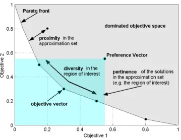
A good representation of a Pareto-optimal set, in terms of DM action, is characterised in three key areas, see [72]. These are illustrated graphically in Figure 1 and listed in the following:
• Proximity: This tells the DM how close the approximation set is to the true Pareto-optimal front. An ideal approximation set should be as close as possible in proximity to the true Pareto-optimal front. In practise, proximity cannot be used as a measure of quality of the approximation set during the optimisation process, because the true Pareto set is not known.
• Diversity: This characterises the distribution of the approximation set both in the extent and uni-formity of that distribution. The ideal approximation set should be uniformly distributed across the trade-o↵surface of the problem.
• Pertinence: This criteria measures the relevance of the approximation set to the DM. Ideally the approximation set should contain a number of solutions which satisfy the DM’s expressed preferences.
Conventional multi-objective optimisation techniques often fail to satisfy these criteria. For example, the goal-attainment method [33] and the weighted-sum method [38] both only provide single solutions to the optimisation problem - thus failing to provide a diverse distribution of solutions. Population based
Figure 1: Proximity, diversity, and pertinence characteristics in an approximation set in two-objective space.
meta-heuristics, such as Evolutionary Multi-Objective Optimisation (EMO) algorithms, are naturally more suitable to tackle multi-objective problems since they process a population of solutions which can then represent the Pareto set, see [22, 44, 54, 64, 78, 94, 97], also when coupled to local search components, e.g. see [77]. Furthermore, population-based algorithms for multi-objective optimisation can be easily endowed with simple and e↵ective components to maintain a diversity of high quality solutions. Recently, in [47], it is proposed a selection mechanism which satisfies at first the diversity of the solutions and then promotes those with the highest proximity. An alternative approach would make use of a mathematical model to generate extra surrogate solutions, e.g. see [13].
A study on the e↵ectiveness of variation in EMO algorithms is reported in [2].
1.1. Many-objective Optimisation
The higher the number of objectives, the more challenging the pairwise comparison of solutions and the subsequent selection process. A multi-objective optimisation problem with more than three objectives is referred to asmany-objective optimisation problem [28], [42, 56].
Analogous to the curse of dimensionality when large scale problems are considered, many-objective problems can introduce challenging difficulties. These challenges have been analysed in the literature, e.g. see [16, 17, 42], and summarised in the following list:
• It is likely that almost all candidate solutions found throughout the optimisation process will be non-dominated, this poses an issue for EMO algorithms which rely on Pareto-dominance for selection pressure, [29, 53, 73].
• The number of candidate solutions required to produce an approximation set which reliably represents the trade-o↵surface increases exponentially [40, 49].
• The number of generations required to produce an approximation set increases, thus making the calculation time of a single run infeasible.
• Search operators become ine↵ective at detecting new non-dominated solutions in the presence of many-objectives [40].
• Approaches which attempt to promote the diversity in the objective space, see [73], can cause issues in terms of convergence, see [84], [58] and [56]. Indeed, convergence and diversity are conflicting in the many-objective case, see [73] and [56].
• The visualisation of candidate solutions becomes difficult, often resulting in the use of heat-maps or parallel-coordinate plots. This poses a difficulty to the DM as the selection of a final candidate solution may become non-intuitive [85].
The transition between the multi-objective problem domain and the many-objective problem domain is not straightforward, such that the methods used to optimise solutions for a multi-objective problem have little to none of the desired e↵ect when applied to a many-objective problem. A fundamental example of this is that the selection mechanisms based dominance that perform well on multi-objective problems (two or three objectives) [18, 20, 79], often do not perform well when four or more problem objectives are considered as shown in [3, 36, 37, 41, 46, 50, 63, 73, 103]. Selection based on dominance is inefficient at producing a strong selection pressure toward the Pareto-optimal front in the presence of many objectives, as throughout the optimisation process it is likely that the entire population will consist of entirely non-dominated solutions. Several alternative algorithmic solutions have been proposed to perform the selection. The following non-exhaustive classification is here proposed.
• Selection methods that use a reference vector. These methods are focussed on the diversity and
ideally aim at achieving an approximation set equally spaced on the Pareto front. In order to achieve this aim, these methods use a reference vector (or weight) and normal distributions to select along each coordinate (in the objective space) the points that are sufficiently distant. A prominent family of algorithms based on this logic consists of the algorithms based on Multi-Objective Evolutionary Algorithm based on Decomposition (MOEA/D) introduced in [95] and initially proposed for multi-objective problems. A further development of the MOEA/D algorithm has been presented in [96] where the MOAE/D with Dynamic Resource Allocation (DRA) has been introduced. MOEA/D-DRA decomposes the many-objective space into multiple single-objective spaces (sub-problems) and then assigns them di↵erent computational budgets. This algorithm, which has been a competition
winner at IEEE CEC is currently one of the most e↵ective and robust solutions at tackling complex multi-objective and at least five-objective problems. Another interesting example of this category is the Non-dominated Sorting Genetic Algorithm III (III) [21, 45]. A further feature of NSGA-III is the use of niching during recombination. This mechanism has been proposed to increase the exploitation of the algorithm. A recent example of an algorithm based on this logic is given in [93]. Another modern example is given in [48] where although a reference vector is used, a diversity-first convergence-second selection strategy.
• Selection methods that divide/classify the population. These methods have the same purpose
of the methods based on reference vectors but achieve this goal by mapping and dividing the objective space. A mapping is then used as a reference to select the points so that they are equally spaced. A historical example in multi-objective optimisation is the Adaptive Grid Algorithm (AGA), see [52], where a grid in the objective space is used to control the population diversity. Another important example is [73] which employed the mechanism to promote diversity. The employment of a grid in the objective space has been reinterpreted and implemented in [60, 91]. Modern studies are reported in [57] where a computationally efficient implementation of a grid-based Pareto approximation is proposed, [58] which is related also to reference vector methods but makes use of distances in the objective space to shift the solutions and guarantee equal spacing, and [56] where the population is structured in multiple layers.
• Selection methods that integrate the DM into the search. These methods bias the selection by
preferring some objectives rather than others. The goal of this approach is to have a high representation of points falling within the ROI. In [98] the direction of the knee points of the Pareto set (those points which represent the lack of a clear preference towards a specific objective) is preferred. This approach shares with [97] the philosophy of avoiding extensive pairwise comparisons and thus handle better large objective spaces. Furthermore, this approach can be seen as a modern re-interpretation of a weighted sum approach where each weight coefficient is set to 1. In [14, 15] the reference vector, i.e. a vector containing the preference weights for each objective, is integrated within the selection process, in order to exclude solutions which do not fall within the ROI from the search. The idea of the incorporation of DM preferences into the algorithmic selection has been proposed in other contexts, e.g. [62, 75, 76].
• Selection methods that make use of indicators. These methods collect other pieces of
informa-tion to extract a scalarized parameter which then assists the selecinforma-tion. An important family is that of Indicator Based Evolutionary Algorithms (IBEAs) [43, 99, 100]. Recently, in [59] a performance comparison indicator to evaluate the quality of approximation sets with the aid of a reference point has been proposed. An interesting indication which does not require any knowledge about the prob-lem is the hypervolume indicator, e.g. see [30]. The hypervolume indicator measures how much of
the objective space is dominated by an approximation set. Although the hypervolume indicator can bias the search towards extremal and knee points of the Pareto, see [59], the way the hypervolume indicator is constructed makes it very appealing in real-world problems. The main attractive point is that this indicator requires no information regarding the theoretical Pareto-front (which in real-world problems is often unknown). Successful examples of incorporating the hypervolume indicator into the optimisation process during the selection process are in [26] and [6] where an adapted version of the hypervolume indicator, named the contributing hypervolume indicator, is used. Other successful cases of the hypervolume used during the selection process are given in [39] and [82] within the context of the Multi-Objective Covariance Matrix Adaptive Evolution Strategy (MO-CMA-ES).
Although the hypervolume indicator is a very valuable sorting criterion for selection, its calculation presents the drawback that it depends exponentially on the number of objectives. Consequently, selection methods incorporating the hypervolume indicator become computationally infeasible in the presence of many-objectives, see [56, 83]. This paper proposes a method to overcome the high computational cost of the hypervolume calculation. This aim is achieved by means of a novel selection mechanism, namely Hypervolume Adaptive Grid Algorithm (HAGA). The proposed HAGA calculates the hypervolume by using only a small set of solutions by using a grid logic inspired by AGA [52]. With the application of HAGA, reliable results in many-objective problems are obtained within a feasible calculation time.
As an analogy, the trade-o↵ between the accuracy of the hypervolume indicator and its computational cost is much like the issues which have been encountered in collision detection in the area of computational physics. The computational cost is due to the accuracy required for collision detection, and the number of objects considered in the simulations. A popular and efficient solution to this issue is the use of a two-phase approach: abroad phase and anarrow phase [66]. The broad-phase is often a crude but computationally fast method of eliminating objects from an object pool which are to be considered for collision detection, in this sense the broad-phase determines which objects do not require further inspection. The narrow phase will then consider the remaining objects for the actual collision detection.
When moving to many-objective problems, optimisation algorithms can benefit from taking inspiration from the two-phase collision detection approach, especially in regards to the computational feasibility of the hypervolume indicator. In a two-phase approach, the contributing hypervolume indicator is well suited for the narrow-phase. An ideal broad-phase algorithm would be computationally lightweight and allow partitioning of the objective space in regards to an approximation set available at each generation of the optimisation process.
In order to have a reasonable computational cost without compromising on the performance of hyper-volume indicator, this paper proposes a novel approach inspired by the collision detection analogy. The proposed method makes use of a two-phase approach to selection which incorporates the contributing
hy-pervolume indicator. The contributing hyhy-pervolume indicator is incorporated such that it is only used to calculate the contributing hypervolume indicator values for sub-populations which are specified by an AGA. In this sense, the proposed approach makes use of an estimation of the hypervolume indicators combined with a population mapping. With this approach, population-wide subjection to the contributing hypervol-ume indicator is avoided and the computational cost of using the contributing hypervolhypervol-ume indicator for achieving selection pressure remains feasible for many-objectives.
The remainder of this article consists of the following sections. Section 2 describes the HV indicator, the related concept of Contributing Hupervolume (CHV) indicator, and the AGA. Section 3 introduces the proposed selection mechanism for many-objective problems. Section 4 provides a full statistical analysis of the results of the proposed novel two-phase approach in comparison to the CHV indicator, and selection by random permutation. Section 5 applies the proposed selection mechanism to a real-world many-objective optimisation problem concerning concealed weapon detection.. Section 6 gives the conclusions of our work, highlights the e↵ectiveness of the proposed approach and its suitability to many-objective optimisation.
2. Background: Hypervolume Indicators and Adaptive Grid Algorithm
2.1. Hypervolume Indicator
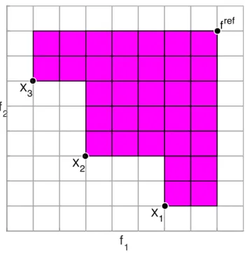
The HV indicator (or s-metric) is a performance metric for indicating the quality of a non-dominated approximation set, introduced by [101] where it is described as the “size of the space covered or size of dominated space”. It can be defined as [82]:
HV fref, X =⇤ [ Xn2X h f1(Xn), f1ref i ⇥· · ·⇥hfm(Xn), fref m i! (1)
whereHV fref, X resolves the size of the space covered by an approximation setX,fref
2Rrefers to a chosen reference point, and⇤(.) refers to the Lebesgue measure [55]. This has been illustrated in Figure 2 in two-dimensional objective space (to allow for easy visualisation) with a population of three solutions.
The Hypervolume (HV) indicator is appealing because it is compatible with any number of problem objectives and requires no prior knowledge of the true Pareto-optimal front, this is important when working with real-world problems which have not yet been solved. The HV indicator is currently used in the field of multi-objective optimisation as both a proximity and diversity performance metric and also in the decision making process [34, 81].
Unlike dominance-based criteria which require only two solutions for performing a comparison (which can be used on an ordinal scale), a reference vector is required to calculate the HV indicator value (i.e. it requires the objective to be measured on an interval scale). When used for pairwise or multiple comparison of optimisation algorithms, this reference vector must be the same, otherwise the resulting HV indicator
f
1f
2 X1 X2 X3 frefFigure 2: An example of the hypervolume indicator in two-dimensional objective space.
values are not comparable. This reference vector can be approximated as large values for each problem objective in order for all objective values in any approximation set to be within the reference vector. A more accurate method for selecting a reference vector, is to use the worst objective values from the union of approximation sets produced on a particular test problem, for each algorithm which is being considered for comparison. This has been described in the following:
8m2 h1, . . . Mi. fref m max D Xm[fref m E (2) where fref
m is the highest value for objectivem in the previous generations of the optimisation process,
andXm is a set of objective values for objectivemfrom the current population. Much e↵ort has been made to speed up the HV calculation, e.g. see [5, 30, 87, 88]
Various implementations of the HV indicator have been presented in [5, 10, 30, 87, 88, 90], all with the aim to speed up its calculation. The HV indicator implementation employed throughout this study is a faster method for exact calculation authored by the Walking Fish Group [87]. The HV indicator has been employed in the performance assessment of algorithms in much of the multi-objective optimisation and evolutionary computation literature (e.g. [24, 36, 67, 74, 80]).
f
1f
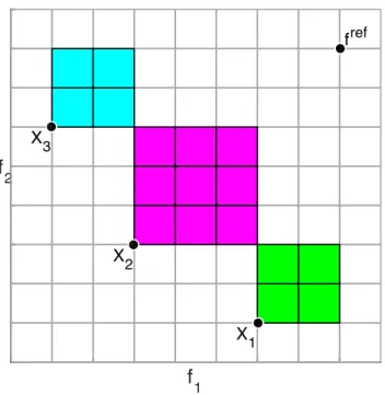
2 X1 X2 X3 frefFigure 3: An example of the CHV indicator in two-dimensional objective space.
2.2. Contributing Hypervolume
The Contributing Hypervolume (CHV) indicator is a population sorting mechanism based on an adap-tation of the HV indicator, see [26], [39], and [6]. The HV indicator works by calculating the size of the objective space that has been dominated by an entire approximation set with respect to a specified reference point, whereas the CHV indicator assigns each solution in an approximation set with the size of the space that has been dominated by each solution exclusively. With this information the population can be sorted by the most dominant and diverse solutions. This has been illustrated in Figure 3 in two-dimensional space with a population of three solutions.
Calculating the exact CHV indicator is attractively simple. The method begins by first calculating the HV indicator quality of a populationX, and then for each solution in the population, the solution is removed and the HV indicator quality is again calculated for the new population. The new HV indicator value is then subtracted from the HV indicator value of the whole population, which results in the CHV indicator value of the solution which was removed. It is then possible to calculate the CHV indicator values of all the
µ+ solutions in the population (µparents and o↵spring), order them by descending value so that they are ordered by the greatest explicit HV indicator contribution, and select the first µsolutions to form the next parent population. This approach has been listed in Algorithm 1.
Although many optimisation algorithms use the CHV as a sorting criterion for selection, its calcula-tion becomes computacalcula-tionally infeasible as the number of objectives considered increases. Monte Carlo
Algorithm 1CHV Indicator execution cycle CHVIndicator(fref, X) 1: XHV HV(fref, X) 2: forn = 1 : do 3: Xt X\Xn 4: HVn HV(fref, Xt) 5: CHVn XHV HVn 6: end for returnCHV
approximations have been used to speed up the calculation of the CHV in [11], which through empirical experiments has shown that the method does not impair the quality of the approximation set. However, the speed increase provided by the Monte Carlo approximation method, still results into an infeasibility of the CHV indicator on problems consisting of five objectives or more.
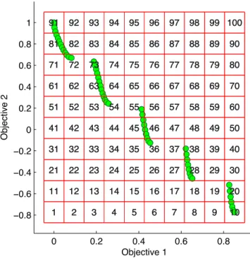
2.3. Adaptive Grid Algorithm
The Adaptive Grid Algorithm (AGA) is a diversity preservation scheme which uses an adaptive grid to keep track of the density of solutions within divisions of the objective space [52]. To achieve this, a grid with a pre-set number of divisions is used to divide the objective space, and when a solution is generated, its grid location is identified and associated with it. Each grid location is considered to contain its own sub-population, and information on how many solutions in the archive are located within a certain grid location is available during the optimisation process, this has been illustrated in Figure 4.
3. A New Selection Mechanism: The Hypervolume Adaptive Grid Algorithm
The proposed Hypervolume Adaptive Grid Algorithm (HAGA) is a selection mechanism consisting of two-phases aiming of being computationally feasible in the presence of many objectives.
HAGA incorporates the use of a novel AGA implementation containing a number of features in order to make the AGA implementation suitable for many-objective optimisation. These novel features consist of:
• A new data structure for storing a solution’s grid number up to any number of problem objectives;
• A new grid-proximity method for grid selection when searching for a solution to remove;
0 0.2 0.4 0.6 0.8 −0.8 −0.6 −0.4 −0.2 0 0.2 0.4 0.6 0.8 1 1 2 3 4 5 6 7 8 9 10 11 12 13 14 15 16 17 18 19 20 21 22 23 24 25 26 27 28 29 30 31 32 33 34 35 36 37 38 39 40 41 42 43 44 45 46 47 48 49 50 51 52 53 54 55 56 57 58 59 60 61 62 63 64 65 66 67 68 69 70 71 72 73 74 75 76 77 78 79 80 81 82 83 84 85 86 87 88 89 90 91 92 93 94 95 96 97 98 99 100 Objective 1 Objective 2 1 2 3 4 5 6 7 8 9 10 11 12 13 14 15 16 17 18 19 20 21 22 23 24 25 26 27 28 29 30 31 32 33 34 35 36 37 38 39 40 41 42 43 44 45 46 47 48 49 50 51 52 53 54 55 56 57 58 59 60 61 62 63 64 65 66 67 68 69 70 71 72 73 74 75 76 77 78 79 80 81 82 83 84 85 86 87 88 89 90 91 92 93 94 95 96 97 98 99 100
Figure 4: An example plot of a population and visualisation of the grid divisions managed by an AGA.
The execution cycle of HAGA is listed in Algorithm 2. With reference to Algorithm 2, HAGA processes an approximation set composed ofµ+ solutions with the aim of selecting µ of them. More specifically, the inputs of HAGA are µ+ vectors of objective values (Xn, with n = 1,2, . . . µ+ ) and the scalar µ
is the number of solutions to be selected. The data structure containing all these vectors is indicated as
X. The output of HAGA is then a new approximation set whose objective values are vectors allocated in a data structureA⇢X composed ofµ solutions. The output approximation set is named parent set and its corresponding solutions are named parent solutions. The notation |X| refers to the cardinality of the populationX.
is a grid location consisting of multiple solutions andCHV t is a vector of entries resulting from the execution of the CHV indicator on the solutions in the grid population t, such that min(CHV t) would resolve the solution which o↵ers the lowest explicit HV indicator contribution in regards to the observed grid population.
In Algorithm 2, Line 5 identifies the grid location closest to the candidate solution and resolves a grid population, the method for which has been described in Section 3.2. This is considered to be the broad-phase of the two-broad-phase approach. Once a grid location has been identified, it is used in the calculation of the narrow-phase (Line 7), which depends on the CHV indicator described in Section 2.2.
The basic principle of HAGA is to benefit from the CHV algorithm’s ability to discriminate solutions based on the explicit HV they contribute to a population, but to do so in a way that doesn’t introduce the
Algorithm 2HAGA execution cycle HAGA(X, µ) =|X| µ 1: forn = 1 : µ+ do 2: if |A|< µthen 3: A A[Xn 4: else
# Where ( n)is the grid location of the maximally populated grid, described in (4).
5: t ClosestGridFromMaximallyPopulated( n)
6: t t[Xn
7: CHV t CHVIndicator( t)
8:
9: # Where min(CHV t)is the solution o↵ering the lowest CHV in the grid. 10: if min(CHV t) =Xn then
11: Discard the candidate solutionXn
12: else
13: Discard min(CHV t) solution
14: A A[Xn
15: end if
16: end if
17: end for
computational infeasibility of using CHV on populations consisting of many-objective solutions.
In order to keep the computational cost feasible, HAGA makes use of the adaptive grid, where the objective space covered by a population is divided into a grid consisting of grid areas. This grid has a capacity for the number of vectors it can store, this capacity is set to µ, which is the number of parent solutions desired for selection. The solutions within the o↵spring are then added to this grid one by one. Throughout this process, there is no computation of the CHV algorithm until the grid reaches capacity. When the capacity is reached (the grid is populated byµ vectors) the inclusion of a new vectorXn must result into the eviction of another vector. In this case, the new vector is temporarily added to the population (which would be temporarily composed of µ+ 1 vectors). Then, a CHV is performed between the newly added vector and all the other solutions belonging to the same sub-population in the grid. With reference to Fig. 5, if we addX4 we would need to apply the CHV forX3, X4, X5 to evict one solution.
This procedure ensures that the CHV is computed for only a small number of solutions. This is done in order to determine which solution is to be evicted from the grid area to prevent the grid from exceeding capacity. In contrast, the CHV algorithm simply computes the CHV indicator value for every solution in the population.
3.1. New Grid Number Data Structure
The mathematical procedure for the proposed AGA structure in its entirety is described herein [52]. M
defines the number of problem objectives and N defines the population size, whilst defines the number of desired grid divisions for a problem objective within the objective space. The data structureX is anM
byN matrix whose generic elementxmn refers to a solution’s objective value:
Xn=hx1n, x2n, . . . , xM ni (3)
is anM byN matrix of entries mn, where every mn refers to the grid location of an objective value xmn in the divided objective space.
n=h 1n, 2n, . . . , M ni (4)
To calculate n, grid location mnof each objective valuexmnfor each solutionXn needs to be resolved.
To calculate a solution’s grid location, the padded grid length⇤, where
⇤=h 1, 2, . . . , Mi (5)
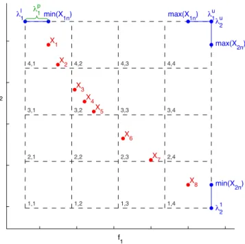
f1 f2 1,1 1,2 1,3 1,4 2,1 2,2 2,3 2,4 3,1 3,2 3,3 3,4 4,1 4,2 4,3 4,4 X1 X2 X3 X4 X5 X6 X7 X8 λ1l min(X1n) max(X1n) λ1u λ21 λ2u min(X2n) max(X2n) λ1p
Figure 5: Illustration of the AGA and its elements on a two-objective approximation-set with = 4.
in the population: p m=| min(Xm) max(Xm)| 2( 1) l m= min(Xm) pm u m= max(Xm) + pm m=| lm um| (6) where l
m is the start point of the grid for objective min the objective space, and um is the end point
of the grid for objectivemin the objective space. These elements have been illustrated in Figure 5. With the grid length and range calculated, it is possible to get the grid location of each solution’s objective value using:
mn= & xmn lm m ' (7)
When the entries of n have been calculated, it can be used to identify the grid location of a solution
Xn. In this new method, the grid location n is defined by a vector rather than a scalar, for example in a five-objective problem a grid location can be described by being at location n=h2,4,1,1,2i.
Grid Number Data Structure Worked-Example
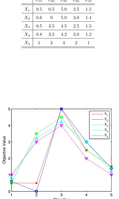
As an example, a populationX of five (N = 5) solutionsXn for a five-objective problem (M = 5) has been presented in Table 1 and Figure 6.
Table 1: An example populationX of objective valuesxmnto be subjected to the proposed AGA scheme. x1n x2n x3n x4n x5n X1 0.5 0.5 5.0 2.5 1.5 X2 0.6 0 5.0 3.0 1.4 X3 0.5 3.5 4.5 2.5 1.5 X4 0.8 3.2 4.2 3.0 1.2 X5 1 3 4 2 1 1 2 3 4 5 0 1 2 3 4 5 Objective Objective Value X 1 X 2 X 3 X 4 X 5
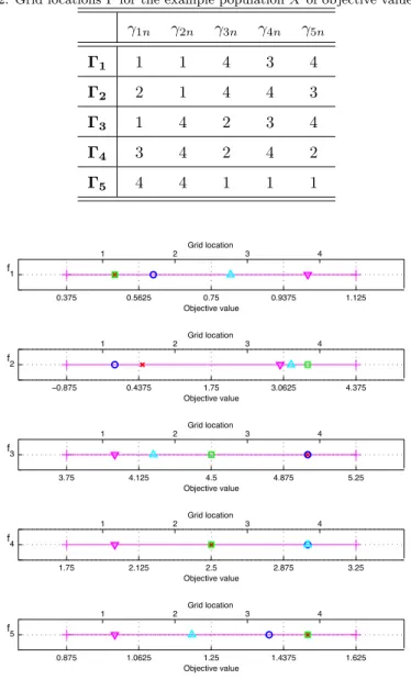
This populationX has been subjected to the proposed AGA scheme to resolve the grid location n of each solutionXn, with an AGA parameter setting of ( = 4) grid divisions. The grid locations resolved by the AGA scheme have been presented in Table 2 and the objective valuesxmn have been plotted in their respective grid locations m in Figure 7, where the plot markers correspond to those used in Figure 6.
Table 2: Grid locations for the example populationXof objective valuesxmn.
1n 2n 3n 4n 5n 1 1 1 4 3 4 2 2 1 4 4 3 3 1 4 2 3 4 4 3 4 2 4 2 5 4 4 1 1 1 0.375 0.5625 0.75 0.9375 1.125 f1 Objective value 1 2 3 4 Grid location −0.875 0.4375 1.75 3.0625 4.375 f2 Objective value 1 2 3 4 Grid location 3.75 4.125 4.5 4.875 5.25 f3 Objective value 1 2 Grid location 3 4 1.75 2.125 2.5 2.875 3.25 f4 Objective value 1 2 3 4 Grid location 0.875 1.0625 1.25 1.4375 1.625 f5 Objective value 1 2 3 4 Grid location
Figure 7: One dimensional plots illustrating the grid locations resolved by the AGA scheme for each objective value, where the plot markers correspond to those used in Figure 6.
The results from this example show that the example population does not consist of any solutions which are in the same grid square (otherwise their entries would be identical).
3.2. Selecting a Solution to Replace
The method for selecting a grid location to remove a solution when the archive is at capacity is important when moving to many-objective problems. Selecting at random from grid locations which are at the same population density increases the probability of causing genetic drift, and decreases the diversity quality of the population. This undesirable e↵ect is scaled exponentially as the number of problem objectives increase, and it is for this reason that many modern EMO algorithms now incorporate a niching approach when concerned with selection [21, 96]. Therefore, it is desirable to find the grid location which is close to both solutions in the objective space and also at a higher density.
Storing grid locations as a single scalar value is not helpful when calculating distance between grid locations or for storing grid locations for a many-objective problem. The grid location structure used in the proposed AGA scheme described above enables an intuitive method for finding the distance between grid locations. By establishing the grid location which a candidate solution would be assigned to, it is possible to find the di↵erence between its grid location and other grid locations which are at high density. This procedure is performed to find out which one it is closest to by summing the di↵erence of the grid location vectors.
Selecting a Solution to Replace Worked-Example
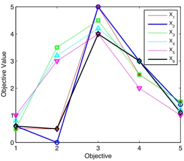
For example, if a new solutionX6=h0.6,0.5,4,3,1.1iwas to be included as a candidate solution as part
of the proposed AGA scheme, it would resolve a grid location of 6=h2,1,1,4,2i. The distance 6between
this grid location ( 6) and the grid locations of the other solutions can be found by finding the absolute di↵erence of each corresponding entry of the candidate solution’s grid location and another solution from the population, and then summing those values.
(i, j) =
M
X
m=1
| m,i m,j| (8)
The distances n between the grid location 6of solutionX6and all the other solutions in the population
presented in Table 1 have been presented in Table 3. The results show that the solution closest in proximity to solutionX6 is solutionX2, this has been visualised in Figure 8.
Table 3: Grid locations for the example populationXof objective valuesxmn.
1 2 3 4 5
6 7 4 8 5 9
Using this method of resolving densely populated grid locations which are closest in proximity to a candidate solution, it is possible to implement the approach listed in Algorithm 3.
1 2 3 4 5 0 1 2 3 4 5 Objective Objective Value X 1 X 2 X 3 X 4 X 5 X 6
Figure 8: Parallel-coordinate plot of the PopulationX used in the proposed AGA example. X6 and the solution closest in
proximity to it,X2, have been presented using thicker lines.
Algorithm 3Closest grid location from maximally populated grid locations
ClosestGridFromMaximallyPopulated( n)
# If the number of grid locations containing the maximal number of solutions exceeds 1 1: if |max( )|>1 then5
# Where maxGammais the set of grid locations containing the maximal number of solutions. 2: for in max( )do
# Calculate the di↵erences between the grid locations # Where n is the equivalent of inmax( )but for n
3: c ( n, )6
4: end for
5: t min( c)
6: else
7: t max( )
# Where max ( ) at this point is the single grid location resolved from the singleton set.
8: end if
return t
5In this case,| |refers to the cardinality of
This algorithm is invoked by Line 5 of Algorithm 2 by ClosestGridF romM aximallyP opulated(Xn). Line 1 checks to see if there is a single grid location which contains the most solutions, if there is more than one grid location that contains the most number of solutions then the algorithm identifies the grid square which is closest in proximity to the candidate solution. nc refers to the di↵erence between the candidate
solution’s grid location and other grid locations, and min( c)refers to the grid location which is the closest in proximity among those containing the maximal number of solutions.
With this feature, it is possible to remove solutions from grid locations which have the highest number of solutions, to make room for solutions in grid locations which have a low number of solutions. This encourages diversity in the overall population.
3.3. Maintaining Extreme Solutions
In previous AGA implementations, the extreme values for each objective were preserved at grid level. In the proposed AGA scheme, solutions containing extreme values for problem objectives (with the candidate solution taken into consideration) are removed from the population before it is subjected to the AGA. No special treatment is given to solutions containing locally (within their grid location) extreme objective values. This ensures candidate solutions are given a better chance of entering the archive than they would have had if they had come up against those solutions containing extreme values. This preserves the overall spread whilst encouraging new solutions to enter the archive.
3.4. Further Remarks
• The proposed HAGA has been designed to be integrated within generational schemes. On steady-state schemes, HAGA would require an extensive calculation at the insertion of each new solution. Consequently, HAGA could result in being computationally expensive when compared to methods employing a di↵erent logic.
• The proposed HAGA, although makes use of a grid, is deeply di↵erent in its logic when compared to grid-based selection mechanisms, see e.g. [91]. While other methods use the grid to select the popu-lation so that it is diverse (in the objective space), the proposed HAGA uses the grid to approximate the calculation of the hypervolume indicator which is then guiding the selection.
4. Numerical Results
The observations made throughout this study have led to the definition of the following testable hy-potheses:
Hypothesis 1. A two-phase approach to selection which incorporates the HV indicator can produce selection
Hypothesis 2. A two-phase approach to selection which incorporates the HV indicator can outperform the CHV indicator in regards to execution time.
Hypothesis 3. A two-phase approach to selection which incorporates the HV indicator can perform
com-parably within a 10% di↵erence in regards to an achieved HV indicator value.
Section 4.1 describes the experimental setup for a number of synthetic test functions used to design test cases for experimentation for the purpose of proving the hypotheses outlined above. The methods of performance assessment have been described in Section 4.2, including the performance metrics employed, the selected sample size, and the use of non-parametric testing. The experiments conclude with an analysis of the results in Section 4.3.
4.1. Experimental setup
In order to test the proposed HAGA selection scheme, the selection process of a generic algorithm generation has been simulated. Our test has been performed on the popular Walking Fish Group (WFG) Tool-kit (WFG1 through to WFG9), see [1, 4, 7, 68, 74]
In order to test the capability of the proposed selection approach to handle very diverse scenarios, this test suite has been used for the proposed method and its competitors, for several levels of dimensionality of the objective space. The test suite has been run using configurations for experiments which consider 2, 3, 5, 10, and 15 objectives.
The selection approaches considered for comparison using these test cases are:
• Selection by Random Permutation(RNDPERM), where a random permutation of the integers
from 1 to (in the case of our experiments, = 200) are generated, and then the firstµ(in the case of our experiments,µ= 100) integers are used as indices for selecting solutions in the population;
• Selection by the Contributed Hypervolume Indicator(CHV) described in Section 2.2 according
to the implementation described in [8, 26], see (1). The population is sorted in descending order by the returned CHV indicator values and the firstµsolutions are selected;
• Selection by the here proposed Hypervolume Adaptive Grid Algorithm(HAGA) according
to the implementation described in Section 3.
In order to compare the performance of the proposed selection approach to the considered alternatives, the experiments are designed around a comparison between the considered selection approaches independent of any host optimisation process. As a result of this, the performance of the considered approaches to selection will not be influenced by external factors. The purpose of these selection approaches is to select a sub-set ofµ(in the case of our experiments,µ= 100) solutions from an existing set of (in the case of our
experiments, = 200) solutions. In the context of an evolutionary algorithm, the population would be the o↵spring population from the previous generational iteration, and theµpopulation would be the parent population which is to be used as parents for evolutionary operators such as recombination.
It must be observed that the Selection by Random Permutation is a naive approach which is based on a simple randomisation. The computational cost of this selection mechanism is expected to be very modest. On the other hand, due to the lack of intelligent and e↵ective components, the performance of this selection scheme is expected to be not too high. The Selection by CHV indicator is a sophisticated mechanism that is likely to o↵er very good performance. Unfortunately, the very high computational cost of this method makes it inapplicable for the many-objective case. Ideally, a selection method for many-objective problems would have the accuracy of CHV and the computational cost of RNDPERM.
The proposed HAGA mechanism attempts to approximate this ideal situation by calculating the CHV indicator only for limited groups of vectors. HAGA is a trade o↵between CHV and RNDPERM philosophies and is here proposed to be a method that, albeit conceptually sophisticated, is computationally cheap and capable of o↵ering very good performance in various multi-objective and many-objective problems.
Of the considered approaches, only HAGA requires a parameter setting, the desired number of grid divisions (which is a discrete parameter).
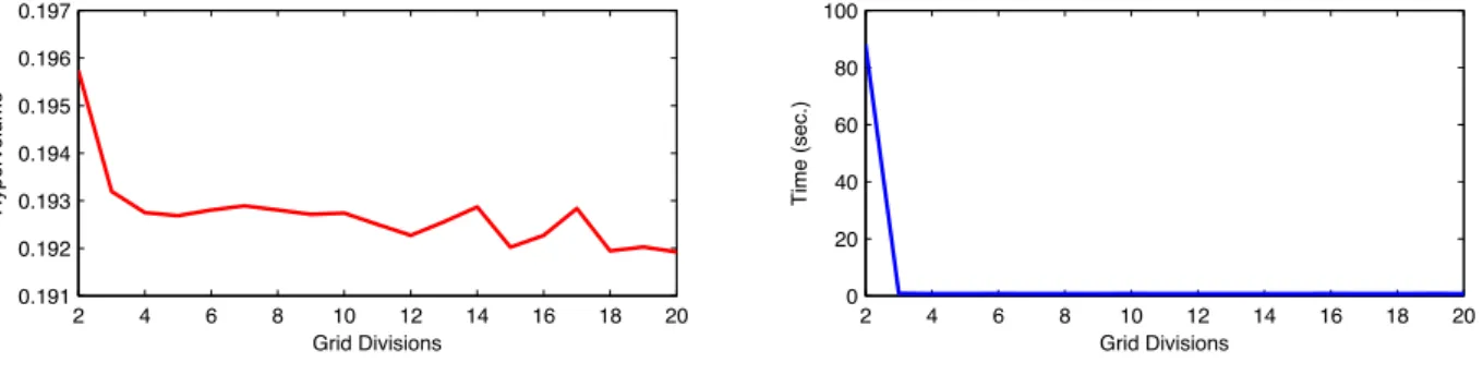
The chosen value of = 3 has been set subsequently to a tuning where the values between 2 and 20 have been taken into consideration, Figure 9 illustrates this exploration for the ten-objective WFG1 test problem. 2 4 6 8 10 12 14 16 18 20 0.191 0.192 0.193 0.194 0.195 0.196 0.197 Grid Divisions Hypervolume 2 4 6 8 10 12 14 16 18 20 0 20 40 60 80 100 Grid Divisions Time (sec.)
Figure 9: The e↵ect of the number of grid divisions ( ) on the Hypervolume performance and execution time of HAGA, demonstrated for the ten-objective WFG1 test problem.
The = 3 setting has been chosen as it proved to give the best performance in terms of computational cost. A lower value of would result in fewer grid squares and therefore larger grid square populations. This will result in worst performance in the computation of the CHV indicator which is used at grid level. In contrast, higher numbers for will result in many more grid locations which may hold only a few
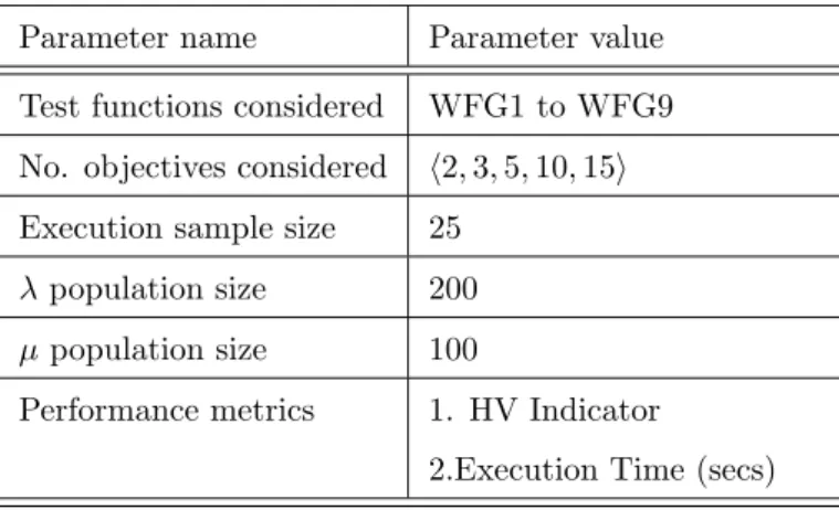
Table 4: Settings used throughout the experiments.
Parameter name Parameter value
Test functions considered WFG1 to WFG9 No. objectives considered h2,3,5,10,15i Execution sample size 25
population size 200
µpopulation size 100
Performance metrics 1. HV Indicator
2.Execution Time (secs)
solutions and often only a single solution. This scenario does not ensure the best performance out of the CHV indicator, as often only a single solution will be subjected to it.
It is important to note that for all problems, e.g. a fifteen-objective problem, although the value of being set to 3 results in 315grid locations available within the grid’s structure, these are only possible grid
locations. The majority of the possible grid locations available in the grid’s structure are not populated because they are located at: dominated areas of the objective space; unpopulated areas of the trade-o↵
surface (either as a result of the design of the objective function or poor diversity); or impossible regions of the objective space. If a grid location does not contain any solutions, it is not considered in any comparisons and no space is reserved for this location during the algorithms execution.
The conditions under which these mechanisms are tested are summarized in Table 4.
Each test case involves using one of the considered approaches for the selection of µindividuals from a population of size , in all our test cases this means selecting the best 100 solutions from a population of 200 solutions. These test cases exist for permutations of all considered problem objectives, test functions, and with 25 samples for each. Each test case uses a unique population of 200 solutions, these solutions have been generated using the competition winning MOEA/D-DRA algorithm (see [96]). The size of the populations produced by MOEA/D-DRA is restricted to 200 by initialising the algorithm with 200 normalised and evenly distributed weights.
This approach to designing test cases and generating sample populations ensured that each considered approach will be subjected to approximation sets consisting of varying proximity and diversity (with a sufficient sample size of 25), for every considered test function, and for every considered problem objective configuration. The HV indicator performs better (in regards to execution time) on some test functions more than others, this di↵erence in performance is not definitively a result of which test function is used, but instead the Pareto-optimal shape produced by solutions to the problem. For this reason it is important that 25 unique samples are used, in particular to evaluate each selection approach on “worst-case” scenarios - as
Table 5: Parameter settings used for the MOEA/D-DRA algorithm used to generate the populations.
Parameter name Parameter value
Niche size 20
Population size 200
Maximum update number 2 Function evaluations 20,000
Table 6: Hardware and software configurations of the computing cluster used to generate the results. Configuration name Configuration value
Architecture Linux-x64
RAM 63 GB
CPU Intel(R) Xeon(R) CPU
E5-2650 @ 2.00GHz⇥16
Total CPU Cores 192
Nodes 16
MATLAB version R2014a 64-bit (glnxa64) Hypervolume Indicator WFG HV 1.0.3
each approach is only as good as its “worst-case” execution in regards to computational cost.
All test cases have been executed on a computing cluster with the configuration listed in Table 6. A computing cluster was required due to the computational cost of executing the CHV indicator on many-objective approximation sets, the same hardware and software was used for all the selection approaches.
4.2. Performance Assessment
Selecting a relevant and sufficient method of performance assessment is a necessity when evaluating or comparing EMO algorithms. These methods of performance assessment can be used to gauge an EMO algorithm’s performance in regards to the proximity, diversity, and pertinence of the final approximation set. Section 4.2.1 describes the performance metrics used to evaluate the considered selection approaches. Section 4.2.2 justifies the sufficiency of the selected sample size for comparison of the considered selection approaches. Section 4.2.3 describes the methods of non-parametric testing employed for the statistical analysis of the selection approaches considered.
4.2.1. Performance Metrics
In order to verify the hypotheses described in Section 4, performance metrics must be employed to resolve the performance of each selection approach considered. Two performance metrics have been considered in this study.
To gauge and compare the performance of a selection approach in selecting a population which achieves a high HV indicator quality, the HV indicatorHV fref, X described in equation (1) (and here synthetically
referred to asHV) has been used as the first performance metric. The HV indicator (described in Section 2.1) is used in conjunction with the reference vectorfref which is generated by taking the worst objective values
from the union of approximation sets produced on a particular test problem after 20,000 function evaluations (calculated using (2)), for each algorithm which is being considered for comparison. This approach to generating the reference point has been chosen to allow a fair comparison amongst all considered hypervolume driven approaches, and to simulate a real-world optimisation scenario where such auxiliary information is often not available before the optimisation process. Through this performance metric the amount of the objective space covered by each selection approach can be observed.
To gauge and compare the performance of a selection approach in regards to its execution time, the MAT-LAB R2014a implementation of the stopwatch timer has been used. This can be achieved using the command “tic;”, followed by the execution of the selection approach, followed by the command “executionT ime =
toc;”. In the following sections of this paper, to keep the notation simple, the cumulative execution time is indicated withT. This cumulative execution time indicates the time taken in seconds by the selection approach on a single CPU thread.
The means and standard deviations for both of the selected performance metrics have been presented in the results section, in order to show the average performance as well as the dispersion of the results.
The CHV indicator can be used to find theµsolutions in a population of size which o↵er the highest possible HV indicator quality, in regards to theµsolutions which score the highest CHV indicator values. This is achieved by selecting the firstµ solutions from an ordered (descending) population based on their CHV indicator values (calculated with Algorithm 1). The lowest possible HV indicator quality which can be achieved byµ solutions from a population of size can also be resolved, in regards to theµ solutions which score the lowest CHV indicator values. This is achieved by selecting the last µ solutions from the same ordered population. By having the worst and best possibleµsolutions in regards to the HV indicator, it is possible to calculate a score indicating the percentage accuracy of a selection approach. The calculation of this score has been defined in Algorithm 4.
This score of accuracy is required as it can be difficult to interpret the magnitude of di↵erence between selection approaches, this is because the magnitude of di↵erence varies from one problem to another, and is heavily dependant on the solutions subjected to the HV indicator. Therefore, the accuracy score will be
Algorithm 4Calculating the HV indicator accuracy
HVIndicatorAccuracy(fref, X, µ, HV)
1: CHV CHVIndicator(fref, X))
2: XU selected from X using firstµCHV indexes 3: XL selected from X using lastµCHV indexes 4: XU HV fref, XU
5: XL HV fref, XL
6: A= HV XL
(XU XL)⇥100
returnA
Hypervolume Indicator Value
0.14 0.16 0.18 0.2 0.22 0.24 Frequency 0 5 10 15 20 25 30 35
40 Distribution of Hypervolume Indicator Values
Figure 10: Histogram showing the distribution of the HV indicator values from 200 executions of MOEA/D-DRA on the WFG6 synthetic test problem.
included in the results for clarity of the di↵erence between the considered selection approaches.
4.2.2. Sample Size Sufficiency
Selecting a sufficient number of samples when comparing optimisers is critical. The sample size of 25, in order to reduce stochastic noise, is re-occurring in the evolutionary computation literature (e.g.[19, 32, 86, 92, 94]). The sufficiency of this sample size has been tested by producing a large number of hypervol-ume indicator value samples by executing MOEA/D-DRA 200 times (the distribution of which has been illustrated in Figure 10) on the WFG6 synthetic test problem.
These 200 samples were then used to identify the relationship between the Standard Error of the Mean (SEM) and the sample size using:
SEM =pSD
N (9)
This relationship has been illustrated in Figure 11 which shows the limited benefit of more than 25 independent executions of the algorithm on the synthetic test problem.
Sample size (N)
0 25 50 75 100 125 150 175 200
Standard Error of the Mean (SEM)
0 0.005 0.01 0.015 0.02 0.025
0.03 Relationship between SEM and N
Figure 11: Relationship between Standard Error of the Mean (SEM) and the sample size of HV indicator values from 200 executions of MOEA/D-DRA on the WFG6 synthetic test problem.
4.2.3. Statistical Set-up
In order to find the significance in contrast amongst the results obtained by algorithms considered for comparison, a non-parametric test (encouraged by [23, 27]) for pairwise statistical comparison has been employed. The Wilcoxon signed-ranks [89] non-parametric test (counterpart of the paired t-test) has been used with the statistical significance value (↵ = 0.05), this is able to rank the di↵erence in performance between two algorithms (pairwise comparisons) over each approximation set.
The Wilcoxon signed-ranks non-parametric test has been employed to contrast the significance of the results generated by the proposed HAGA selection approach to every other considered selection approach, in regards to both the HV indicator and execution time performance metrics. These statistics will allow greater confidence in the verification of the hypotheses described in Section 4.
The choice of the use of a non-parametric test is experimentally justified by the fact that the data are not normally distributed. The latter statement has been shown by means of the one sample Kolmogorov-Smirnov test with the statistical significance value (↵= 0.05).
Furthermore, in order to strengthen the statistical significance of the results presented and have a general statistical sense of the significance of the algorithms across all problems, the Holm-Bonferroni procedure has been applied with confidence level of 0.05, see [35], [32], and [31].
Both Wilcoxon tests and Holm-Bonferroni procedure have been applied twice per each algorithm in order to evaluate the quality of the results and the time required to achieve them. The quality is expressed as the Hypervolume metricHV and cumulative execution time (CPU-time)T.
4.3. Results
This section presents the numerical results considered in this study. For each algorithm and each test problem, the average values of the HV indicatorHV and the±standard deviations are reported in Table 7. In the same table, average values of the calculation time with the corresponding standard deviation values are also displayed. In Table 7 the number of objectives under consideration is indicated with M. In the following table, a higher mean HV indicator value denoted byHV indicates greater performance in regards to area of the objective space dominated. In contrast, a lower mean execution time value denoted byT indicates greater performance in regards to the time taken to complete the execution for a selection approach, meaning the greater performance indicates less time taken.
The HV indicator valuesHV have been normalised to avoid the generation of large numbers and to allow for better comparison between selection approaches. The method of normalisation used has been defined in (10).
HV =QMHV
m=1frefm
(10)
With this method of normalisation, the mean HV indicator valuesHV will always reside between 0 and 1.
The results of the Wilcoxon signed-ranks test have also been included in Table 7, where a ’+’ indicates that the null hypothesis was rejected, and the HAGA selection approach displayed statistically superior performance at the 95% significance level (↵= 0.05) on the considered test case. A ’ ’ indicates that the null hypothesis was rejected, and the HAGA selection approach displayed statistically inferior performance. An ’=’ indicates that there was no statistically significant di↵erence between both of the considered selection approaches on the considered test case.
Table 8 displays the results of the Holm-Bonferroni procedure in terms of both the hypervolume indicator
HV and the execution timeT.
It can be observed that HAGA has intermediate features with respect to CHV and RNDPERM. As expected, CHV always returns the best HV value with respect to because it performs a search over all the possible values. In contrast, RNDPERM always has the worst HV performance, and thus never outperforms the proposed selection approach (HAGA). Furthermore, the intermediate performance of HAGA is much closer to CHV performance than to the RNDPERM performance as displayed in Table 7, although HAGA performance on the HV cannot outperform the extensive search performed by CHV.
Regarding the execution time performance, it can be immediately observed that the three methods em-ploy di↵erent logics with very di↵erent computational costs, especially when the complexity of the methods with respect to the dimensionality of the objective space is considered. Since RNDPERM simply performs random permutations it is computationally very cheap and its cost does not depend on the dimensionality
Ta b le 7 : M ea n v a lu es ± standard dev iation v alues of h y p erv olume indicator and calculation time for R A N DP E R M , CH V , and H A GA . A v a lue in b old indicates the highest p erforming approac h for the corresp onding p erformance metric. A greater H V score indicates greater H V indicator p erformance, an d a lesser T score indicates fas ter p er fo rmance. R N D PER M CHV HA GA M Fn HV ± T ± HV ± T ± HV ± T ± 2 WF G1 0 . 26103 ± 0 . 01048 = 0.00089 ± 0.00010 – 0.26261 ± 0.01083 = 0 . 01396 ± 0 . 00648 – 0 . 26261 ± 0 . 01084 0 . 21728 ± 0 . 10040 2 WF G2 0 . 63461 ± 0 . 01615 = 0.00087 ± 0.00007 – 0.63628 ± 0.01622 = 0 . 00759 ± 0 . 00428 – 0 . 63622 ± 0 . 01623 0 . 05468 ± 0 . 00986 2 WF G3 0 . 63135 ± 0 . 00609 + 0.00090 ± 0.00007 – 0.63572 ± 0.00581 = 0 . 01944 ± 0 . 00713 – 0 . 63460 ± 0 . 00753 0 . 36607 ± 0 . 07442 2 WF G4 0 . 46150 ± 0 . 00478 + 0.00084 ± 0.00006 – 0.46533 ± 0.00468 = 0 . 01147 ± 0 . 00475 – 0 . 46529 ± 0 . 00457 0 . 06388 ± 0 . 01354 2 WF G5 0 . 44960 ± 0 . 00223 + 0.00086 ± 0.00006 – 0.45342 ± 0.00186 = 0 . 02302 ± 0 . 00923 – 0 . 45319 ± 0 . 00194 0 . 41180 ± 0 . 05766 2 WF G6 0 . 49072 ± 0 . 00836 + 0.00087 ± 0.00007 – 0.49440 ± 0.00834 = 0 . 02138 ± 0 . 00742 – 0 . 49418 ± 0 . 00830 0 . 57747 ± 0 . 06463 2 WF G7 0 . 50823 ± 0 . 00497 + 0.00088 ± 0.00008 – 0.51239 ± 0.00444 = 0 . 01388 ± 0 . 00476 – 0 . 51235 ± 0 . 00442 0 . 25407 ± 0 . 07760 2 WF G8 0 . 44568 ± 0 . 00535 = 0.00088 ± 0.00008 – 0.44944 ± 0.00538 = 0 . 01462 ± 0 . 00599 – 0 . 44843 ± 0 . 00597 0 . 23082 ± 0 . 06540 2 WF G9 0 . 49869 ± 0 . 00482 + 0.00086 ± 0.00007 – 0.50237 ± 0.00431 = 0 . 01595 ± 0 . 00645 – 0 . 50195 ± 0 . 00443 0 . 32247 ± 0 . 11638 R N D PER M CHV HA GA M Fn HV ± T ± HV ± T ± HV ± T ± 3 WF G1 0 . 34652 ± 0 . 01176 = 0.00086 ± 0.00006 – 0.35109 ± 0.01223 = 0 . 15059 ± 0 . 00890 – 0 . 35036 ± 0 . 01253 0 . 59704 ± 0 . 04166 3 WF G2 0 . 81993 ± 0 . 01605 = 0.00086 ± 0.00006 – 0.82707 ± 0.01454 = 0 . 11019 ± 0 . 00946 – 0 . 82688 ± 0 . 01454 0 . 42262 ± 0 . 04688 3 WF G3 0 . 58817 ± 0 . 00993 + 0.00087 ± 0.00009 – 0.59665 ± 0.00981 = 0 . 11637 ± 0 . 00874 – 0 . 59614 ± 0 . 01125 0 . 52284 ± 0 . 04523 3 WF G4 0 . 54612 ± 0 . 01508 + 0.00085 ± 0.00006 – 0.56339 ± 0.01269 = 0 . 11447 ± 0 . 01082 – 0 . 56026 ± 0 . 01301 0 . 33683 ± 0 . 04832 3 WF G5 0 . 56191 ± 0 . 01090 + 0.00087 ± 0.00008 – 0.57983 ± 0.00689 = 0 . 15198 ± 0 . 00758 – 0 . 57434 ± 0 . 00965 0 . 53927 ± 0 . 03212 3 WF G6 0 . 60525 ± 0 . 00811 + 0.00084 ± 0.00005 – 0.61545 ± 0.00996 = 0 . 16443 ± 0 . 00732 – 0 . 61525 ± 0 . 00834 0 . 60009 ± 0 . 02691 3 WF G7 0 . 55759 ± 0 . 01213 + 0.00085 ± 0.00006 – 0.57357 ± 0.01148 = 0 . 13220 ± 0 . 00936 – 0 . 56834 ± 0 . 01256 0 . 46005 ± 0 . 05513 3 WF G8 0 . 50919 ± 0 . 01250 + 0.00086 ± 0.00008 – 0.52295 ± 0.01162 = 0 . 13297 ± 0 . 00937 – 0 . 52137 ± 0 . 01184 0 . 45089 ± 0 . 05183 3 WF G9 0 . 58318 ± 0 . 01089 + 0.00088 ± 0.00009 – 0.59875 ± 0.00941 = 0 . 13620 ± 0 . 01184 – 0 . 59536 ± 0 . 00946 0 . 48412 ± 0 . 05889 R N D PER M CHV HA GA M Fn HV ± T ± HV ± T ± HV ± T ± 5 WF G1 0 . 35384 ± 0 . 00489 + 0.00085 ± 0.00006 – 0.35604 ± 0.00495 = 1 . 65278 ± 0 . 16109 + 0 . 35599 ± 0 . 00495 0 . 78154 ± 0 . 10825 5 WF G2 0 . 84441 ± 0 . 01309 = 0.00088 ± 0.00010 – 0.84972 ± 0.01316 = 1 . 18229 ± 0 . 15747 + 0 . 84966 ± 0 . 01317 0 . 75523 ± 0 . 13534 5 WF G3 0 . 52060 ± 0 . 00915 = 0.00088 ± 0.00009 – 0.53367 ± 0.00777 – 0 . 67558 ± 0 . 07894 + 0 . 52522 ± 0 . 01116 0 . 56657 ± 0 . 03422 5 WF G4 0 . 60365 ± 0 . 01257 + 0.00086 ± 0.00007 – 0.63447 ± 0.01208 = 1 . 11964 ± 0 . 09373 + 0 . 62973 ± 0 . 01319 0 . 44297 ± 0 . 04703 5 WF G5 0 . 63766 ± 0 . 01701 + 0.00088 ± 0.00007 – 0.67332 ± 0.01543 = 1 . 36957 ± 0 . 07382 + 0 . 66853 ± 0 . 01631 0 . 57354 ± 0 . 03647 5 WF G6 0 . 70205 ± 0 . 01062 + 0.00085 ± 0.00005 – 0.72360 ± 0.00946 = 1 . 50883 ± 0 . 23307 + 0 . 72322 ± 0 . 01302 0 . 59686 ± 0 . 02849 5 WF G7 0 . 56674 ± 0 . 01387 + 0.00088 ± 0.00006 – 0.59519 ± 0.01190 = 1 . 33294 ± 0 . 10874 + 0 . 59138 ± 0 . 01479 0 . 53652 ± 0 . 03597 5 WF G8 0 . 50688 ± 0 . 01941 + 0.00087 ± 0.00009 – 0.53508 ± 0.02046 = 1 . 17091 ± 0 . 12492 + 0 . 53255 ± 0 . 02056 0 . 46476 ± 0 . 05669 5 WF G9 0 . 63646 ± 0 . 01386 + 0.00088 ± 0.00009 – 0.66422 ± 0.01396 = 1 . 25577 ± 0 . 09913 + 0 . 65887 ± 0 . 01413 0 . 54510 ± 0 . 03100
R N D PER M CHV HA GA M Fn HV ± T ± HV ± T ± HV ± T ± 10 WF G1 0 . 20132 ± 0 . 00333 = 0.00084 ± 0.00007 – 0.20261 ± 0.00323 = 1944 . 52962 ± 531 . 90048 + 0 . 20253 ± 0 . 00325 1 . 20437 ± 1 . 25042 10 WF G2 0 . 81638 ± 0 . 02935 = 0.00085 ± 0.00009 – 0.82305 ± 0.02876 = 379 . 51965 ± 216 . 71658 + 0 . 82292 ± 0 . 02854 0 . 83236 ± 0 . 53270 10 WF G3 0 . 36728 ± 0 . 01762 + 0.00083 ± 0.00006 – 0.39405 ± 0.01654 = 245 . 89231 ± 208 . 88644 + 0 . 38837 ± 0 . 01741 0 . 68271 ± 0 . 02954 10 WF G4 0 . 52966 ± 0 . 02916 + 0.00084 ± 0.00005 – 0.57416 ± 0.02744 = 1561 . 46369 ± 559 . 03596 + 0 . 56968 ± 0 . 02868 0 . 49096 ± 0 . 07500 10 WF G5 0 . 47830 ± 0 . 02242 + 0.00085 ± 0.00006 – 0.54329 ± 0.02461 = 2448 . 10859 ± 818 . 45709 + 0 . 53862 ± 0 . 02456 0 . 65928 ± 0 . 03369 10 WF G6 0 . 68586 ± 0 . 01854 + 0.00083 ± 0.00006 – 0.71780 ± 0.01744 = 1032 . 64211 ± 453 . 56564 + 0 . 71643 ± 0 . 01901 0 . 58623 ± 0 . 06133 10 WF G7 0 . 46453 ± 0 . 02266 + 0.00083 ± 0.00006 – 0.50875 ± 0.01732 = 2188 . 14782 ± 756 . 95283 + 0 . 50482 ± 0 . 01700 0 . 59102 ± 0 . 04497 10 WF G8 0 . 39281 ± 0 . 03009 + 0.00083 ± 0.00004 – 0.44048 ± 0.02385 = 988 . 63944 ± 442 . 54752 + 0 . 43631 ± 0 . 02313 0 . 44876 ± 0 . 05142 10 WF G9 0 . 47978 ± 0 . 03400 + 0.00083 ± 0.00003 – 0.52364 ± 0.03176 = 1653 . 95165 ± 508 . 52791 + 0 . 51589 ± 0 . 03149 0 . 59211 ± 0 . 03683 R N D PER M CHV HA GA M Fn HV ± T ± HV ± T ± HV ± T ± 15 WF G1 0 . 05828 ± 0 . 00083 = 0.00082 ± 0.00003 – 0.05879 ± 0.00083 = 907721 . 87235 ± 503090 . 31807 + 0 . 05871 ± 0 . 00080 0 . 85870 ± 0 . 19637 15 WF G2 0 . 67912 ± 0 . 05525 = 0.00082 ± 0.00003 – 0.69114 ± 0.05205 = 26611 . 33190 ± 25193 . 59089 + 0 . 69113 ± 0 . 05203 0 . 85797 ± 0 . 34234 15 WF G3 0 . 14061 ± 0 . 02104 + 0.00082 ± 0.00003 – 0.16198 ± 0.01944 = 7091 . 19596 ± 13241 . 35130 + 0 . 16113 ± 0 . 01967 0 . 75482 ± 0 . 02921 15 WF G4 0 . 47475 ± 0 . 03276 + 0.00083 ± 0.00004 – 0.52097 ± 0.03117 = 701963 . 39534 ± 378065 . 47797 + 0 . 51678 ± 0 . 03041 0 . 59002 ± 0 . 05213 15 WF G5 0 . 38401 ± 0 . 02065 + 0.00082 ± 0.00002 – 0.44142 ± 0.01504 = 119015 . 48008 ± 204799 . 57140 + 0 . 43516 ± 0 . 01571 0 . 74370 ± 0 . 02826 15 WF G6 0 . 56713 ± 0 . 04370 + 0.00082 ± 0.00003 – 0.61667 ± 0.04145 = 161766 . 09125 ± 188396 . 91632 + 0 . 61407 ± 0 . 03985 0 . 58675 ± 0 . 09660 15 WF G7 0 . 35930 ± 0 . 01814 + 0.00082 ± 0.00003 – 0.41198 ± 0.01766 = 347654 . 60867 ± 529981 . 05882 + 0 . 40279 ± 0 . 01988 0 . 67919 ± 0 . 04909 15 WF G8 0 . 33059 ± 0 . 02538 + 0.00082 ± 0.00003 – 0.38010 ± 0.01967 = 151056 . 00468 ± 169033 . 02908 + 0 . 36997 ± 0 . 01853 0 . 83264 ± 1 . 19337 15 WF G9 0 . 31253 ± 0 . 02062 + 0.00082 ± 0.00002 – 0.36172 ± 0.02264 = 303512 . 07185 ± 280140 . 17679 + 0 . 35640 ± 0 . 02137 0 . 71350 ± 0 . 04720
Table 8: Holm-Bonferroni procedure
j Method Rank zj pj /j
HV value (reference: HAGA, Rank = 2.02e+00)
1 CHV 3.00e+ 00 4.64e+ 00 < e 05 5.00e 02 HA 2 RND 1.02e+ 00 4.74e+ 00 < e 0.5 2.50e 02 HA
T value (reference: HAGA, Rank = 1.60e+00)
1 RND 3.00e+ 00 6.64e+ 00 < e 05 2.50e 02 HA
2 CHV 1.40e+ 00 0.95e+ 00 0.17e00 5.00e 02 H0
of the objective space.
On the contrary, CHV performs a HV check of all the entire set of solutions. Analogous to what happens in single-objective optimisation when the dimensionality of the decision space is scaled up, the size of objective space exponentially grows with the number of objectives. Hence, the computational cost of CHV heavily depends on the number of objectives of the problem and grows exponentially with it. As shown in Table 7, the computational cost of CHV is very modest in the two-objective case. In the three-objective case the computational cost of CHV is about ten times higher than for a two-objective problem. In the five-objective case, the cost of CHV is over a second which may be already approaching a limitation for real-time applications (taking into account that a many-objective optimisation algorithm requires thousands of CHV selections). For a higher dimensionality of the objective space, the cost of CHV is very high making CHV unusable, or at least not very attractive. It can be observed that for a fifteen-objective problem a single CHV selection may require more than ten calculation days.
The proposed HAGA selection approach performs a search and has a non-null computational cost. Fur-thermore, the computational cost of HAGA depends on the number of objectives of the problem. However, its computational cost does not grow exponentially with the size of the objective space. On the contrary, the computational cost of HAGA grows extremely slowly when compared to the computational cost of CHV and is around, or within, a second for all of the problems considered in this study. Furthermore, HAGA appears to reliably o↵er a fairly highHV performance with a modest computational cost. In terms of its computational behaviour, HAGA can be regarded as a surrogate assisted strategy, e.g. see [61] and [69], that operates in the multi-dimensional objective space. For example a population selection for WFG1 for fifteen objectives can be solved by HAGA more than five million times faster that CHV selection still attaining a very good approximation of the theoretical HV accuracy (0.05871 instead of 0.05879), see Table 7.
These features make the proposed HAGA selection approach attractive for real-world application which require the solution of many-objective problems in a reasonable time.
Figure 12 depicts the computational cost depending on the number of objectives for the three selection schemes under consideration. It must be noted that in order to make the di↵erence in cost between CHV and the other methods visible, the plot is represented in logarithmic scale. The trend displayed in Figure
Figure 12: Computational cost (T) of RNDPERM, CHV, and HAGA (logarithmic scale).
12 can be seen as a complexity analysis where the scalability is studied in the objective space instead of in the decision space.
Figure 13 depicts the HV indicator accuracy depending on the number of objectives for the three selection schemes under consideration. The HV indicator accuracy has been resolved using the procedure listed in Algorithm 4 in order to o↵er a normalised measure of performance between the considered selection approaches. The CHV selection approach scores each solution in the population based on the explicit area of the objective space which it dominates, with these scores it is possible to identify either the combination of solutions which cover the most objective space, and also the combination of solutions which cover the least of the objective space. With these two populations which dominate the most and least of the objective space, it is possible to use the HV indicator in each of them to resolve the worst achievable HV indicator score and the best achievable HV indicator score for the test case under consideration. It is possible to assume that any combination ofµsolutions based on CHV indicator values from the population will score somewhere between these upper and lower achievable HV indicator values, and with this knowledge it is possible to arrive at a normalised (between 0 and 1) measure of performance of the considered selection approaches across all considered test cases. This HV indicator accuracy can also be seen as a percentage, whereby a HV indicator accuracy of 0% indicates the worst possible combination ofµ solutions and a HV indicator accuracy of 100% indicates the best possible combination of µ solutions in regards to the HV indicator.
It can be observed in Figure 13 that the CHV selection approach scores a consistent HV indicator accuracy of 1 (or 100%), this is to be expected as theoretically the CHV indicator by design is able to order a population based on explicit domination of the objective space. The RNDPERM selection approach is shown to achieve a mean HV indicator accuracy of 0.7 (or 70%), with the lowest HV indicator accuracy scoring at 0.67 (or
Figure 13: Hypervolume Accuracy (A) of RNDPERM, CHV, and HAGA.
67%), this is an expected and undesirable score. If the RNDPERM approach to selection was employed throughout an optimisation process, it can be assumed that at each generation a new parent population of sizeµwould be selected from the o↵spring population of size , and that this new parent population would consist of solutions that on average represent 70% of the objective space which can be dominated by the o↵spring population. It can therefore be assumed that many of the solutions forming this new o↵spring population are: solutions which are dominated by other solutions in the o↵spring population; solutions which o↵er very little in terms of explicit contribution to the HV indicator; or identical solutions which o↵er nothing to the quality of the new parent population. Through this process of using the RNDPERM selection approach, it is possible that the HV indicator quality of populations resolved at each generation oscillate, or regress due to the lack of selection pressure. The HAGA selection approach is shown to achieve a mean HV indicator accuracy of 0.966 (or 96.6%), with no HV indicator accuracy score below 0.957 (or 95.7%), this performance remains consistent from problems consisting of two problem objectives up to at least fifteen problem objectives. An average HV indicator accuracy score of 96.6% suggests that regardless of the number of considered problem objectives, the HAGA approach to selection is able to o↵er great selection pressure towards dominant areas of the objective space.
4.4. Comparison against another approximated HV indicator
In order to to further prove the efficiency of the proposed HAGA, we have compared it with another selection method for many-objective optimisation based on an approximated estimation of the hypervolume indicator, i.e. HypE reported in [6]. The same experiments as above have been repeated and HAGA has the same parameters used in the previous sections. Regarding HypE, its parameter has been set to achieve an error of only 1% as suggested in its paper: number of samples 105. Table 9 displays the results of this