Hierarchical Classification Using Evolutionary Strategy

40

© Global Society of Scientific Research and Researchers

http://asrjetsjournal.org/

Hierarchical Classification Using Evolutionary Strategy

Helyane Bronoski Borges

*, Julio Cesar Nievola

, Simone Nasser Matos

Jardim Carvalho, Ponta Grossa, 84017-220, Parana, Brazil b

Pontifical Catholic University of Paraná (PUCPR), Address Imaculada Conceição, 1155 - Prado Velho, Curitiba, 80215-901, Parana, Brazil

a

Email: [email protected] b_{Email: [email protected]}

c_{Email: [email protected]}

Abstract

Hierarchical classification is a problem with applications in many areas as protein function prediction where the dates are hierarchically structured. Therefore, it is necessary the development of algorithms able to induce hierarchical classification models. This paper presents experimenters using the algorithm for hierarchical classification called Hierarchical Classification using Evolutionary Strategy (HC-ES). It was tested in eight datasets the G-Protein-Coupled Receptor (GPCR) and Enzyme Commission Codes (EC). The results are compared with other hierarchical classifier using the distance and hF-Measure.

Keywords: Hierarchical Classification; Evolutionary Strategy; Classifier.

1.Introduction

Hierarchical classification is a task of data mining that has been applied in diverse areas such as the music prediction, images [1], text [2], among others [3,4,5]. In bioinformatics, it has been used for functional prediction of proteins, since this is not an easy task to accomplish without the help of efficient techniques [6]. The prediction of protein functions can be treated as a classification problem in data mining, in which proteins attributes are considered a sample in the database and its biological functions as classes (multi-class classifiers). Most algorithms for hierarchical classification of proteins have been developed to support class hierarchies with a tree structure [7, 8], but the use of ontology in predicting protein functions has been used as in the case of Gene Ontology (GO) [3,4].

--- * Corresponding author.

41

In this paper an algorithm for hierarchical classification of data for structures such as tree are developed denominated of HC-ES (Hierarchical Classification Using Evolutionary Strategy) is applied. The experiments are focuses on hierarchical protein function prediction using G-Protein-Coupled Receptor (GPCR) and Enzyme Commission Codes (EC) [8].

2.Hierarchical Classification

The hierarchical classification differs from flat classification because the classes are organized in a hierarchy structured as a tree or a DAG (Directed Acyclic Graph) where the nodes of this hierarchy represent the classes that are involved in the classification process [9]. The main difference between the tree structure and the DAG structure is that in the tree structure each node (each class), except the root node, has only one ancestor (parent), while in the DAG structure each node (class) may have one or more ancestors’ nodes. Another characteristic that makes flat classification different from hierarchical classification refers to the prediction type of classes in the hierarchy, which can be distinguished into two categories: mandatory leaf node prediction (possible in flat or hierarchical classification) and non-mandatory leaf node (possible only in hierarchical classification) [9]. In mandatory leaf node prediction all examples should be associated with classes represented by leaf nodes. In the non-mandatory leaf node prediction there is no requirement that the prediction occurs at leaf nodes. Thus, the examples may be associated with classes that are represented by any internal node of the class hierarchy along with their ancestors. To explore hierarchical classification problems some solutions have been proposed, which can be divided into three main approaches: flat hierarchical classification, local hierarchical classification and global hierarchical classification. These approaches describe how the classifiers are built and not a classification method, such as top-down approach that is often cited in literature as being one of the approaches [3,9]. The hierarchical classification a class is represented by a vertex of this hierarchy. Thus, when an input example predicts that the sample is associated with a particular class, automatically this example will also be classified as belonging to all its ancestor classes. The root node corresponds to "any class" showing a total lack of knowledge of the class of an object.

3.Proposed Approach: Hierarchical Classification Using Evolutionary Strategy (HC-ES)

The HC-ES algorithm consists in training a global hierarchical classifier based on the evolutionary strategy using the approach (μ + λ) [10]. This classification approach has the advantage of evaluating the predictive performance of the entire class hierarchy, reporting a single result. This proposed classifier has three steps: initialization, training and test algorithms.

3.1.Initialization HS-SE Algorithm

The initialization process of the HS-ES algorithm is realized using an input the training database (DBTrain) and the hierarchical class (CH). The size individual’s or chromosome population (p) is informed. An instance ei of input data set DBTrain = {{e1}, {e2},..., {eq}} is formed by a sample set eq being q size database. Each element of DBTrain consists of attributes e1{a1, a2,...,ali} are the class attributes (ali) and li-1 is the amount of attributes. CH = {c1,c2,..., cc} is formed by a set of class hierarchy and c is the amount class hierarchy. PI =

42

{pi1, pi2,..., pigene} are individuals, where gene is number of class that exists in the class hierarch and P = {PI1,PI2,…, PIgene} is individual’s set. Figure 1 show the population set (P) getting by of the initialization according p where the size individual or chromosome pi is an element.

... ... ... ... ... ... ... ... ...

... ... ... ... ...

... ... ... ... ... ... ... ... ...

... ... ... ... ... ... ... ... ...

... ... ... ...

Individual’s or Chromosome Population

P

o

p

u

la

tio

n

(

P

)

.

.

.

p

p

.

.

.

Figure 1: Creating Population (P)

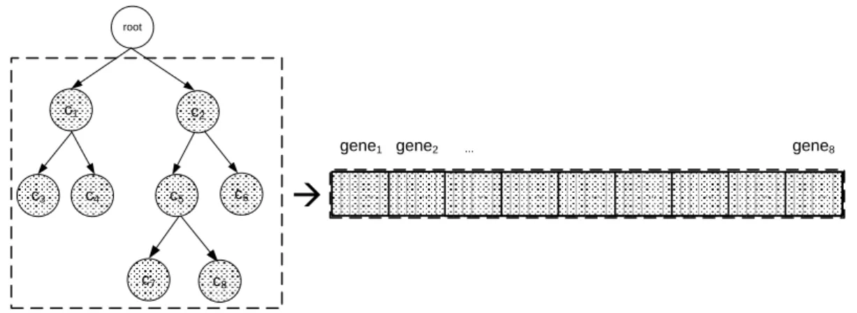
The size chromosome gene is relationship with the amount hierarchical class, ie, in Figure 2 show eight class gene = c = 8 (c1,c2,...,c8), therefore the chromosome size is eight.

root c2 c6 c8 c1 c4 c5 c3 c7 ... ... ... ... ... ... ... ... ...

à

gene1 gene2 ... gene8

Figure 2: Transformation of the class hierarchical in an individual of the HC-ES

3.2.Train HS-ES Algorithm

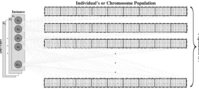
The next step is training HS-ES algorithm. An instance ei of the database DBTrain is selected randomize (see Figure 3). After is calculate the Euclidean distance between each input instance with all individuals in the population. Further, it is obtaining the fitness of each individual (hit rate of each individual).

43

.

.

.

.

.

.

Individual’s or Chromosome Population

P o p u la tio n ( P ) Instance e1 e2 eq . . .

Figure 3: Example of the training process.

The individual’s fitness is evaluate using the measure approach Distance-based Depth-Dependent Measures. When evaluating the result of a hierarchical prediction three situations may occur: correct prediction, partially correct prediction and incorrect prediction. Each of these situations will be exemplified.

4.Correct Prediction

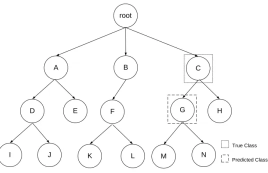
There are two types of possible correct prediction. The first one occurs when the algorithm hits the full path, being the predicted class equal to the true class as shown in Figure 4 (The true class is “G” and the predicted class is “G”). A D C root E B F G H K L N I _M True Class Predicted Class J

Figure 4: Example of Correct Prediction - 1st Possibility

The second case occurs when the predicted class is in the full path of the correct one, but it is more specific. Figure 5 shows this possibility: the true class is represented by the node "C" in the tree, and the algorithm predicts the node "G". This case is considered a correct prediction.

44

Figure 5: Example of Correct Prediction - 2nd Possibility

5.Partially Correct Prediction

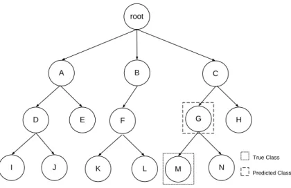
An example of a partially correct prediction is shows in Figure 6. In this case, the true class is represented by the node "L" but the algorithm predicts the class represented by the node "G". Observe that the node's parent node is predicted true. Although the predicted class is in the correct path it stops before finding the more detailed true class in the tree, not providing the full specificity of it. Therefore, one can say that the prediction was partially correct, because the algorithm was on the correct path of prediction, it just occurred before hitting the full specification. An instance, whose class is predicted at higher levels, tends to be more easily classified than a class in deeper levels. Thus, the algorithm considers it a partial prediction, being based on the level of class, which means, classes at levels closer to the root have higher importance than classes at deeper levels. In this example, the class is predicted on the second level and true class is at the third level. Then, indices of importance are assigned inversely proportional to the level of the classes, i.e., the class "G" is replaced by an index two times larger than the class "L". Equation 1 shows the formula for this calculation

1p+2p+…+np=1 (1)

where p is the index and n is the level in the hierarchy. The correct prediction rate is the sum of weights of classes correctly predicted, i.e. the predicted class and its ancestor classes. Applying the equation to this example p = 0.16. Thus, the weight of class "M" is 0.16, and the class "G" is 0.33 and the class "C" is 0.5. Then the hit rate of this sample is 83%.

45

Figure 6: Example of Partially Correct Prediction

6.Incorrect Prediction

There is an incorrect prediction when the predicted class totally misses the path prediction as shown in Figure 7. It is observed that the true class is represented by the node "C", however, the algorithm predicts incorrectly the class as "D". A D C root E B F G H K L N I M True Class Predicted Class J

Figure 7: Example of Incorrect Prediction

Based on fitness the individuals are selected by the roulette method and the sequence can be applied recombination and mutation. Recombination is calculated as follows: two individuals are selected father1 and father2. These two individuals will give rise to two descendants’ individual child1 and child2. The calculation of recombination are shows in Equation 2.

child1 = (father1 * c + (father2 * (1 - c))

child2 = (father1 * (1 – c)) + (father2 * c

(2)

46

Later, these individuals will be applied to mutation [10]. The mutation applied in HC-ES algorithm used a factor mutation for all individuals. Table 1 presents the HC-ES training algorithm.

Table 1: Training of HC-ES Algorithm

INPUT

- Training data set DBTrain=[e1 e2 e3 … eq] of dimension q.

- Class hierarchy CH.

STEP 1: INITIALIZE

- Determine the population size P.

- Determine number of generations G.

- Initialize the P constituted by individuals PI that are represented by PI=[pi1, pi2, pi3,…,pigene].

STEP 2: STOPPING CRITERION

- Number of G.

STEP 3: TRAINING

- Select an instance ei of the input data set DBTrain=[e1,e2,e3,eq].

- Calculate the distance between the instance ei with all individuals in the population.

- Obtain the fitness of each individual.

- Applied Roulette Method in the individuals selected by fitness.

- Applied Recombination based in the Equation 2.

- Applied to Mutation.

OUTPUT

- Population of individual adequate.

6.1.Test HS-ES Algorithm

The procedure for testing the algorithm is similar to the training procedure. The main difference is that at this stage the individual population are fixed from the last generation of the training step. Two evaluation measures were used to report the predictive performance of the samples: distance-based depth-dependent measure and hierarchy based measures [11]. The choice of these measures was made to assess the performance of the classification in different ways.

7.Experiments and results

47

protein G-Protein-Coupled Receptor (GPCR) and the other four formed by Enzyme Commission Codes (EC). These sets were available from the authors of the work [8]. Table 2 shows some characteristics of these databases. For the all experiments 2/3 of the examples were used for training and 1/3 for testing (hold-out procedure). In addition, all sets were normalized using the approach Min-Max. Na observation to be made is that some nodes of the hierarchy have only a few children, which causes a great unbalance in the tree [3]. The constant c of the Equation 2 is used the value is 0.7.

Table 2: Characteristics of Databases

Databases Samples Attributes Class Class by level

ECinterproFinal 14036 1216 331 6/41/96/188 ECpfamFinal 13995 708 334 6/41/96/191 ECprintsFinal 14038 382 352 6/45/92/209 ECprositeFinal 14048 585 324 6/42/89/187 GPCRinterproFinal 7461 450 198 12/54/82/50 GPCRpfamFinal 7077 75 192 12/52/79/49 GPCRprintsFinal 5422 282 179 8/46/76/49 GPCRprositeFinal 6261 128 187 9/50/79/49

The experiments were done using three values for number of generations: 20, 60 and 100, with a population of 50 individuals.

7.1.Results of Experiments

The results are presented based on distance-based depth dependent measure (Dist) and hF-Measure (hF). The Table 3 shows the results obtained by HC-ES algorithms in the 20, 60 and 100 generations.

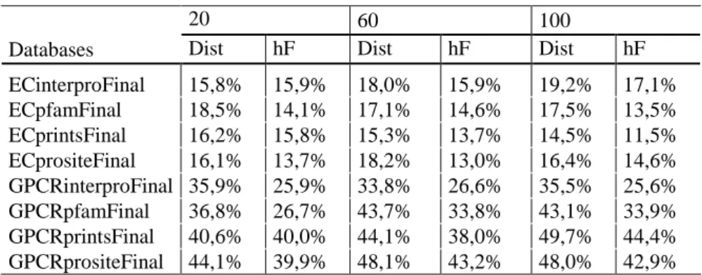
Table 3: Results obtained by HC-ES algorithms

20 60 100

Databases Dist hF Dist hF Dist hF

ECinterproFinal 15,8% 15,9% 18,0% 15,9% 19,2% 17,1% ECpfamFinal 18,5% 14,1% 17,1% 14,6% 17,5% 13,5% ECprintsFinal 16,2% 15,8% 15,3% 13,7% 14,5% 11,5% ECprositeFinal 16,1% 13,7% 18,2% 13,0% 16,4% 14,6% GPCRinterproFinal 35,9% 25,9% 33,8% 26,6% 35,5% 25,6% GPCRpfamFinal 36,8% 26,7% 43,7% 33,8% 43,1% 33,9% GPCRprintsFinal 40,6% 40,0% 44,1% 38,0% 49,7% 44,4% GPCRprositeFinal 44,1% 39,9% 48,1% 43,2% 48,0% 42,9% 7.2.Results Comparation

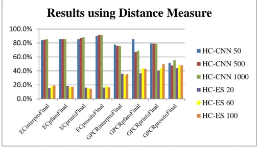
The results were statistically compared using the Friedman [12, 13,14] test to verify whether there is statistical significance between the differences the performances of the algorithms. The Figure 8 shows the comparison of the HC-CNN [2] e HC-ES algorithms when applied the distance measure. Analyzing the results statistically with 95% significance level, it is observed that the HC-CNN algorithm with 1000 cycles is statistically superior

48

to the results of HC-ES algorithm in the three selected cases 20, 60 and 100 generations. Moreover, HC-CNN algorithm with 50 and 500 cycles is statistically higher than the HC-ES execution of 20 generations.

Figure 8: Comparison of the HC-CNN e HC-ES algorithms when applied the distance measure

Figure 9 shows the comparison of the HC-CNN e HC-ES algorithms when applied the hF measure. Statistically analyzing the results, it is observed that there is a statistical difference between the results of the algorithms.

Figure 9: Comparison of the HC-CNN e HC-ES algorithms when applied the hF measure.

The HC-CNN algorithms when applied 1000 cycles superior to the results of HC-ES algorithm in the three selected cases 20, 60 and 100 generations. Therefore, the HC-CNN algorithms with 50 cycles is statistically higher than the HC-ES execution of 20 generations.

8.Conclusion

This paper presented a new global hierarchical classifier that using evolutionary strategy called HC-ES, for prediction of structured data in tree. This classification approach has the advantage of evaluating the predictive

0.0% 20.0% 40.0% 60.0% 80.0% 100.0%

Results using Distance Measure

HC-CNN 50 HC-CNN 500 HC-CNN 1000 HC-ES 20 HC-ES 60 HC-ES 100 0.0% 20.0% 40.0% 60.0% 80.0% 100.0%

Results using hF-Measure

HC-CNN 50 HC-CNN 500 HC-CNN 1000 HC-ES 20 HC-ES 60 HC-ES 100

49

performance of the entire hierarchy class, reporting a single result. The results of the predictions were assessed using two approaches to hierarchical classification measures: distance-based depth-dependent measure and hF-Measure. The HC-ES algorithm presented results statically below when compared with the HC-CNN algorithm. However, these are the first experiments with HC-ES algorithm. Other experiments with the HC-ES classifier should be realized using others amount of individuals and the generation to analyze the predictive performance the algorithm.

References

[1]. Dimitrovski, I. et al. “Hierarchical classification of diatom images using ensembles of predictive clustering trees”. Ecological Informatics, Elsevier, vol. 7, pp. 19-29, 2012.

[2]. Baraldi, P. et al. “Hierarchical k-nearest neighbours classification and binary differential evolution for fault diagnostics of automotive bearings operating under variable conditions”. Engineering Applications of Artificial Intelligence, vol. 56, pp. 1–13, 2016.

[3]. Borges, H. B.; Silla, C. N.; Nievola, J. C. “An evaluation of global-model hierarchical classification algorithms for hierarchical classification problems with single path of labels”. Computers & Mathematics with Applications, vol. 66, pp. 1991-2002, 2013.

[4]. Vens, C. et al. “Decision trees for hierarchical multi-label classification. Machine Learning”. Springer, vol. 73, pp. 185–214, 2008.

[5]. Xu, H.; Yang, W.; Wang, J. “Hierarchical emotion classification and emotion component analysis on Chinese micro-blog posts”. Expert systems with applications, vol. 42, pp. 8745–8752, 2015.

[6]. Secker, A. et al. “Hierarchical classification of g-protein-coupled receptors with data-driven selection of attributes and classifiers”. International journal of data mining and bioinformatics, vol. 4, pp. 191– 210, 2010.

[7]. Borges, H. B.; Nievola, J. C. “Hierarchical classification using a Competitive Neural Network”, In Proc. of the Eighth International Conference on Natural Computation (ICNC), 2012, pp. 172-177. [8]. Holden N, Freitas A. “Hierarchical classification of protein function with ensembles of rules and

particle swarm optimization”. Soft Computing, vol. 13, pp. 259–272, 2009.

[9]. Silla, C.; Freitas, A. A. “A survey of hierarchical classification across different application domains”. Data Mining and Knowledge Discovery, vol. 22, pp. 31-72, 2011.

[10]. Bäck, T.; Fogel, D. B.; Michalewicz, Z. Evolutionary computation 2: advanced algorithms and operators. Bristol and Philadelphia: Institute of Physics Publishing, 2000.

[11]. Kiritchenko, S. et al. “Learning and evaluation in the presence of class hierarchies: application to text categorization”, in Proc. of the 19th Canadian Conf. on Artificial Intelligence, Lecture Notes in Artificial Intelligence, 2006, pp. 395-406.

[12]. Friedman, M. “The use of ranks to avoid the assumption of normality implicit in the analysis of variance”. Journal of the American Statistical Association, vol. 32, pp. 675–701, 1937.

[13]. Friedman, M. “A comparison of alternative tests of significance for the problem of m rankings’. In: Annals of Mathematical Statistics, vol. 11, pp. 86–92, 1940.

[14]. Desmar, J. “Statistical comparisons of classifiers over multiple data sets”. Journal of Machine Learning Research, vol. 7, pp. 1-30, 2006.